Filling Gaps in Chaotic Time Series

Abstract

We propose a method for filling arbitrarily wide gaps in deterministic time series. Crucial to the method is the ability to apply Takens’ theorem in order to reconstruct the dynamics underlying the time series. We introduce a functional to evaluate how compatible is a filling sequence of data with the reconstructed dynamics. An algorithm for minimizing the functional with a reasonable computational effort is then discussed.

One problem faced by many practitioners in the applied sciences is the presence of gaps (i.e. sequences of missing data) in observed time series, which makes hard or impossible any analysis. The problem is routinely solved by interpolation if the gap width is very short, but it becomes a formidable one if the gap width is larger than some time scale characterizing the predictability of the time series.

If the physical system under study is described by a small set of coupled ordinary differential equations, then a theorem by Takens Takens80 ; Embedology91 suggests that from a single time series is possible to build-up a mathematical model whose dynamics is diffeomorph to that of the system under examination. In this paper we leverage the dynamic reconstruction theorem of Takens for filling an arbitrarily wide gap in a time series.

It is important to stress that the goal of the method is not that of recovering a good approximation to the lost data. Sensitive dependence on initial conditions, and imperfections of the reconstructed dynamics, make this goal a practical impossibility, except for some special cases, such as small gap width, or periodic dynamics. We rather aim at giving one or more surrogate data which can be considered compatible with the observed dynamics, in a sense which will be made rigorous in the following.

I Introduction

We shall assume that an observable quantity $s$ is a function of the state of a continuous-time, low-dimensional dynamical system, whose time evolution is confined on a strange attractor (that is, we explicitly discard transient behavior). Both the explicit form of the equations governing the dynamical system and the function which links its state to the signal $s(t)$ may be unknown. We also assume that an instrument samples $s(t)$ at regular intervals of length $\Delta t$, yelding an ordered set of $\bar{N}$ data

$$s_{i}=s\left((i-1)\Delta t\right),\,\,\,i=1,\ldots,\bar{N}.$$ (1)

If, for any cause, the instrument is unable to record the value of $s$ for a number of times, there will be some invalid entries in the time series $\{s_{i}\}$, for some values of the index $i$.

From the time series $\{s_{i}\}$ we reconstruct the underlying dynamics with the technique of delay coordinates. That is, we shall invoke Takens’ theorem Takens80 ; Embedology91 and claim that the $m$-dimensional vectors

$$\mathbf{x}_{i}=\left(s_{i},s_{i+\tau},\ldots,s_{i+(m-1)\tau}\right)$$

lie on a curve in $\mathbb{R}^{m}$ which is diffeomorph to the curve followed in its (unknown) phase space by the state of the dynamical system which orginated the signal $s(t)$. Here $\tau$ is a positive integer, and $i$ now runs only up to $N=\bar{N}-(m-1)\tau$. Severals pitfalls have to be taken into account in order to choose the most appropriate values for $m$ and $\tau$. Strong constraints also come from the length of the time series, compared to the characteristic time scales of the dynamical system, and from the amount of instrumental noise which affects the data. We shall not review these issues here, but address the reader to references Theiler86 ; NoisyReconstruction91 ; Provenzale92 .

We note that gaps (that is, invalid entries) in the time series $\{s_{i}\}$ do not prevent a successful reconstruction of a set $\mathcal{R}=\{\mathbf{x}_{i}\}$ of state vectors, unless the total width of the gaps is comparable with $\bar{N}$. We simply mark as “missing” any reconstructed vector $\mathbf{x}_{i}$ whose components are not all valid entries.

If the valid vectors of $\mathcal{R}$ sample well enough the underlying strange attractor embedded in $\mathbb{R}^{m}$, one may hope to find, by means of a suitable interpolation technique, a vector field $\mathbf{F}:U\rightarrow\mathbb{R}^{m}$ , such that within an open set $U$ of $\mathbb{R}^{m}$ containing all the vectors $\mathbf{x}_{i}$, the observed dynamics can be approximated by

$$\dot{\mathbf{x}}=\mathbf{F}(\mathbf{x}).$$ (2)

This very idea is at the base of several forecasting schemes, where one takes the last observed vector $\mathbf{x}_{N}$ as the initial condition for equation (2), and integrates it forward in time (see e.g., FarmerSidorowich87 ; Casdagli89 ).

The gap-filling problem was framed in terms of forecasts by Serre et. al. Serre92 . Their method, which amounts to a special form of the shooting algorithm for boundary value problems, is limited by the predictability properties of the dynamics, and cannot fill gaps of arbitrary width.

The rest of this note is organized as follows: in section II we cast the problem as a variational one, where a functional measures how well a candidate filling trajectory agrees with the vector field defining the observed dynamics. Then an algorithm is proposed for finding a filling trajectory. In section III we give an example of what can be obtained with this method. Finally, we discuss the algorithm and offer some speculations on future works in sec. IV.

II A variational approach

The source of all difficulties of gap-filling comes from the following constraint: the interpolating curve, which shall be as close as possible to a solution of (2), must start at the last valid vector before the gap and reach the first valid vector after the gap in a time $T$ which is prescribed.

To properly satisfy this constraint, we propose to frame the problem of filling gaps as a variational one. We are looking for a differentiable vector function $\xi:[0,T]\rightarrow U$ which minimizes the continuous functional

$$J(\xi)=\int_{0}^{T}\left\|\dot{\xi}(t)-\mathbf{F}\left(\xi(t)\right)\right\|^{2}dt,$$ (3)

with

$$\xi(0)=\mathbf{x}_{p};\,\xi(T)=\mathbf{x}_{q}.$$

Defining $l=q-p$, we have $T=l\,\Delta t.$ If the curve $\xi(t)$ coincided with the missing curve $\mathbf{x}(t)$ for $t\in[0,T]$, and $\mathbf{F}$ where a perfect reconstruction of the vector field governing the dynamics of the system, then the functional would reach its absolute minimum $J=0$. The imperfect nature of $\mathbf{F}$ suggests that any curve which makes $J$ small enough can be considered, on the basis of the available information, a surrogate of the true (missing) curve. In section III we shall offer a simple criterion to quantify how small is “small enough”. For the moment we only care to remark that, even for a perfect reconstruction of the vector field, a curve $\xi$ making $J$ abitrarily small, but not zero, need not to approximate $\mathbf{x}(t)$, in fact, the two curves may be quite different; however, such a curve $\xi$ is consistent with the dynamics prescribed by (2).

Most methods for minimizing functionals focus on approaching as quickly as possible the local minimum closest to an initial guess. Because we may confidently assume that $J$ has many relative minima far away from zero, we expect that these algorithms will fall on one of these uninteresting minima for most choices of the initial guess. Thus, our problem really reduces to that of finding a suitable initial guess.

The complexity of the problem is greatly limited if we require that the set $\mathcal{L}=\{\mathbf{y}_{j}\}$, whose $l+1$ elements sample the initial guess, has to be a subset of the set $\mathcal{R}$ of reconstructed vectors. The index $j=0,1,\ldots,l$ does not necessarily follow the temporal order defined in $\mathcal{R}$ by the index $i$ (cfr. eq. (1)), but we require that $\mathbf{y}_{0}\equiv\mathbf{x}_{p}$ and $\mathbf{y}_{l}=\mathbf{x}_{q}$. We shall denote with $S(\mathbf{y}_{j})$ the successor of the vector $\mathbf{y}_{j}$ with respect to the temporal order in $\mathcal{R}$, and with $P(\mathbf{y}_{j})$ its predecessor. We propose that a good choice for the set $\mathcal{L}$ is one which makes as small as possible the following discretized form of the functional $J$:

$$J_{0}\left(\{\mathbf{y}_{j}\}\right)=\sum_{j=1}^{l-1}\left|\mathbf{y}_{j+1}-\mathbf{y}_{j-1}-S(\mathbf{y}_{j})+P(\mathbf{y}_{j})\right|^{2}.$$ (4)

Of course, we shall restrict our choice of vectors to be included in $\mathcal{L}$ only to valid vectors of $\mathcal{R}$ having valid predecessor and successor. $J_{0}$ could be zero if and only if $\mathcal{L}$ cointained all the missing vectors in the correct order: $\mathcal{L}=\{\mathbf{x}_{p},\mathbf{x}_{p+1},\ldots,\mathbf{x}_{q}\}$. The value of $J_{0}$ increases every time that the order according to the $j$-index is different from the natural temporal order, that is, every time that $S(\mathbf{y}_{j})\neq\mathbf{y}_{j+1}$ or $P(\mathbf{y}_{j})\neq\mathbf{y}_{j-1}$. If this happens we say that there is a jump in $\mathcal{L}$ between, respectively, the position $j$ and $j+1$, or $j$ and $j-1$.

Although a set $\mathcal{L}$ which performs many very small jumps may conceivably attain a very low value of $J_{0}$, there is an exceedingly small probability to find it within a finite dataset. An intuitive demonstration of this statement comes from the histogram in figure 1, which shows the distribution of distancies between each reconstructed vector and its closest neighbor for the dataset discussed in section III: as expected the frequency of closest neighbors quickly drops to zero for short distancies. Then our strategy will be that of looking for a set $\mathcal{L}$ which performs as few jumps as possible.

Let us call orbit any sequence of valid vectors which does not jump. The first vector of an orbit shall have a valid predecessor, and the last a valid successor. Thus we define the predecessor of the orbit as the predecessor of its first vector and likewise the successor of the orbit as the successor of its last vector. We say that an orbit is consecutive to a point if its successor or its predecessor is the closest neighbor of the point. Two orbits are consecutive if the successor of one orbit is the closest neighbor of the first vector of the other orbit, or if the predecessor of one orbit is the closest neighbor of the last vector of the other orbit. Let us call branch a set made of consecutive orbits. Below we describe a simple algorithm to construct a set $\mathcal{L}$ by joining together one or more consecutive orbits.

1. We follow forward in time the orbit consecutive to $\mathbf{x}_{p}$ for $l$ steps, or until it has a valid successor. We store away the set of points made of $\mathbf{x}_{p}$ followed by the points of this orbit as the $1$-jump forward branch.

2. For each point $\mathbf{y}_{j}$ of each $(n-1)$-jumps forward branch (where $j=r,2r,\ldots\,\leq l_{f}$, $r$ is an arbitrary stride, $l_{f}+1$ is the number of points in the forward branch, and $l_{f}\leq l$,), we follow forward in time the orbit consecutive to $\mathbf{y}_{j}$ for $l-j$ steps, or until it has a valid successor. We store away all the points up to $\mathbf{y}_{j}$ of the current forward branch followed by the points of the consecutive orbit as one of the $n$-jumps forward branches.

3. We repeat step 2 for a fixed number $n_{f}$ of times.

4. We follow backward in time the orbit consecutive to $\mathbf{x}_{q}$ for $l$ steps, or until it has a valid predecessor. We store away the points of the consecutive orbit followed by $\mathbf{x}_{q}$ as the $1$-jump backward branch.

5. For each point $\mathbf{z}_{j}$ of each $(n-1)$-jumps backward branch (where $j=r,2r,\ldots\,\leq l_{b}$, $r$ is an arbitrary stride, $l_{b}+1$ is the number of points in the backward branch, and $l_{b}\leq l$), we follow backward in time the orbit consecutive to $\mathbf{z}_{j}$ for $j$ steps, or until it has a valid predecessor. We store away all the points of this orbit followed by all the points from $\mathbf{z}_{j}$ to the end of the current backward branch as one of the $n$-jumps backward branches.

6. We repeat step 5 a fixed number $n_{b}$ of times.

7. For all possible pairs made by one forward branch and one backward branch we examine synchronous pairs of points, that is a point $\mathbf{y}_{j_{f}}$ in the forward branch, and a point $\mathbf{z}_{j_{b}}$ in the backward branch such that $j_{f}+l_{b}-j_{b}=l$, where $l_{b}+1$ is the number of points in the backward branch. If they coincide, or one is the closest neighbour of the other, then we define $\mathcal{L}=\{\mathbf{y}_{0},\ldots,\mathbf{y}_{j_{f}},\mathbf{z}_{j_{b}+1},\ldots,\mathbf{z}_{l_{b}+1}\}$.

The presence of jumps in $\mathcal{L}$ makes it unsuitable as a filling set for the gap. Furthermore, the discretized form (4) of the functional (3) is meaningful only if its arguments $\{\mathbf{y}_{j}\}$ are a subset of the set of reconstructed vectors $\mathcal{R}$. Then we need a different discretization of (3) which allows as argument any point of $U$. The simplest among many possibilities relies on finite differences, leading to the following expression

$$J_{1}\left(\{\mathbf{w}_{j}\}\right)=\sum_{j=1}^{l}\left[\frac{\mathbf{w}_{j}-\mathbf{w}_{j-1}}{\Delta t}-\mathbf{F}(\mathbf{w}_{j-1/2})\right]^{2}$$ (5)

where the vectors $\mathbf{w}_{j}$ may or may not belong to $\mathcal{R}$, and $j=0,1,\ldots,l$. Here $\mathbf{F}(\mathbf{w}_{j-1/2})$ is the vector field $\mathbf{F}$ evaluated at the midpoint between $\mathbf{w}_{j-1}$ and $\mathbf{w}_{j}$. $J_{1}$ is a function of $m(l-1)$ real variables ($\mathbf{w}_{0}=\mathbf{w}_{p}$ and $\mathbf{w}_{l+1}=\mathbf{w}_{q}$ shall be kept fixed), which can be minimized with standard techniques, using $\mathcal{L}$ as the initial guess.

III An example

In this section we show how the algorithm described above performs on a time series generated by a chaotic attractor. We numerically integrate the Lorenz equations Lorenz63 with the usual parameters ($\sigma=10$, $r=28$, $b=8/3$). We sample the $x-$variable of the equations with an interval $\Delta t=0.02$, collecting $5000$ consecutive data points which are our time series. One thousand consecutive data points are then marked as “not-valid”, thus inserting in the time series a gap with a width of 1/5th of the series length, corresponding to a time $T=20$. For this choice of parameters the Lorenz attractor has a positive Lyapunov exponent $\lambda\approx 0.9$ Froyland83 , setting the Lyapunov time scale at $\lambda^{-1}\approx 1.1$. We also find that the autocorrelation function of the time series drops to negligible values in about 3 time units. We conclude that $T$ is well beyond any realistic predictability time for this time series.

In the present example we selected the embedding delay $\tau=5$ simply by visual inspection of the reconstructed trajectory, and we choose an embedding dimension $m=3$. However, we checked that results are just as satisfactory up to (at least) embedding delay $\tau=15$, and embedding dimension $m=6$.

We apply the algorithm with $n_{f}=2$ and $n_{b}=0$. The strides are $r=1$ for the 2-jumps forward orbits and $r=100$ for the 3-jumps forward orbits. This leads to 11001 forward orbits to be compared with 1 backward orbit, looking for synchronous pairs points which are neighbour of each other. We find two such pair of points, and the corresponding two initial guesses $\mathcal{L}_{1}$ and $\mathcal{L}_{2}$ are such that $J_{0}(\mathcal{L}_{1})=1.21$ and $J_{0}(\mathcal{L}_{2})=1.04$.

The approximating vector field $\mathbf{F}$ is extremely simple, and its choice is dictated solely by ease of implementation. A comparison between different interpolating techniques is off the scope of this paper, and the interested reader may find further information in Casdagli89 . If $\bar{\mathbf{x}}_{j}$ and $\bar{\bar{\mathbf{x}}}_{j}$ are the vectors of $\mathcal{R}$, respectively, closest and second closest to $\mathbf{w}_{j}$, then we define

$$\mathbf{F}(\mathbf{w}_{j-1/2})=\frac{\bar{\mathbf{x}}_{j}-P(\bar{\mathbf{x}}_{j})+\bar{\bar{\mathbf{x}}}_{j}-P(\bar{\bar{\mathbf{x}}}_{j})}{2\Delta t}.$$ (6)

Using the definition (6) in (5), we obtain $J_{1}(\mathcal{L}_{1})=3.46$ and $J_{1}(\mathcal{L}_{2})=3.17$. In order to smooth-out the jumps in the filling sets, the function $J_{1}$ is further decreased by iterating five times a steepest-descent line minimization (see, e.g., NumRecipesII ) using $\mathcal{L}_{1}$ and $\mathcal{L}_{2}$ as initial guesses. This procedure yelds two sets of $l+1$ points, $\mathcal{M}_{1}$ and $\mathcal{M}_{2}$ such that $J_{1}(\mathcal{M}_{1})=1.54$, and $J_{1}(\mathcal{M}_{2})=1.34$. The corresponding time series are shown in figure 2. The difference between the smoothed sets $\mathcal{M}_{1}$ and $\mathcal{M}_{2}$ plotted in figure 2 and the sets with jumps $\mathcal{L}_{1}$ and $\mathcal{L}_{2}$ would be barely noticeable on the scale of the plot.

The effect of the smoothing may be appreciated by looking at figure 3 which shows the region across the jump between two consecutive orbits of $\mathcal{L}_{1}$. The non-smoothed filling set (dashed line) abruptly jumps from one orbit to the other, but the smoothed trajectory (thick solid line) singled out by the points of $\mathcal{M}_{1}$ gently moves between them.

No attempt has been made to approach as closely as possible the local minimum of $J_{1}$. In fact, we verified that for orbits in $\mathcal{R}$ having the same length as the interpolating sets $\mathcal{M}_{1}$ and $\mathcal{M}_{2}$, $J_{1}$ ranges (roughly) between 1 and 9. This is a measure of the accuracy with wich the field $\mathbf{F}$ approximates the true dynamics of the observed system, and there is no point in looking for an interpolating set having a value of $J_{1}$ below this range.

IV Discussion and conclusions.

In this note we have described an algorithm which fills an arbitrarily wide gap in a time series, provided that the dynamic reconstruction method of Takens is applicable. The goal is to provide a filling signal which is consistent with the observed dynamics, in the sense that, in the reconstructed phase space, the vector tangent to the filling curve should be close to the vector field modeling the observed dynamics. This request is cast as a variational problem, defined by the functional (3). The acceptable degree of closeness is determined by the level of accuracy of the reconstruction, which we quantify by computing the discretized form (5) of the functional for orbits having the same length of the gap.

Obviously, if the time series has more than one gap, our method can be applied to all the gaps, indipendently from each other.

A second novel idea, that greatly simplyfies the problem, is that of building a rough solution by stitching together pieces of the observed dataset. The actual solution, which will not be an exact copy of anything present in the observed dataset, is obtained by refining this first draft. We have illustrated a basic algorithm that embodies this idea, although no attempt has been made at making it computationally optimal. In particular, with the algorithm in its present form, many of the forward and backward branches will be partial copies of each other, because nothing forbids two distinct branches to jump on the same orbit. This leaves some room for improvement, because the effectiveness of the method relies on a substantial amount of the set $\mathcal{R}$ of reconstructed vectors to be explored by a relatively limited number of branches. In a forthcoming, enhanced version of the algorithm some kind of tagging mechanism shall be incorporated in order to produce non-overlapping hierarchies of forward and backward branches.

We observe that this algorithm does not give a guarantee of success: it is perfectly possible that no point of the forward branches is the closest neighbor of (or coincides with) a synchronous point of the backward branches. In this case the obvious attempt is to deepen the hierarchy of the branches, as much as it is computationally feasible. Or, one may relax the request that branches may jump only between closest neighbors, and accept jumps between second or third neighbors as well. As a last resort, one may stitch any pair of forward and backward branches at their closest synchronous points, hoping that the resulting jump could later be smoothed satisfactorily by minimizing the function (5). However, when facing a failure of the algorithm, we believe that first should be questioned the goodness and appropriateness of the dynamic reconstruction. The presence of too many gaps, the shortness of the time series, or measurement inaccuracies may make the gap-filling problem an insoluble one. We speculate that the ability of filling gaps with relative ease is a a way to test the goodness of a dynamic reconstruction.

The ease with which a gap may be filled, as a function of his width, is a problem deserving further work. For the moment we simply recall that if a set of initial conditions of non-zero measure is evolved in time according to (2), eventually we expect it to spread everywhere on the attractor (here the measure is the physical measure $\mu$ of the attractor cfr. ref. EkRue85 ). More rigorously, if $\phi_{t}$ is the flow associated to (2), and if it is a mixing transformation, then, for any pair of sets $A$, $B$ of non-zero measure, $\lim_{t\rightarrow\infty}\mu(\phi_{t}A\cap B)=\mu(A)\mu(B)$. The dispersion of a set of initial conditions is further discussed in Sklar73 , where, for example, it is shown that the essential diameter of a set of initial conditions cannot decrease in time, after an initial transient of finite length.

This leads to the idea that wide gaps should be easier to fill than not-so-wide ones, because forward and backward branches have explored larger portions of the attractor, and so there is a greater chance to find synchronous points where they can be joined together. As a first step toward the verification of this hypotesis, we computed the average minimum distance between synchronous points of the 1-jump forward and backward branch as the gap moves along the dataset, for several gap widths. We used the dataset discussed in sec. III and a ten times longer extension of it. The results, plotted in figure 4, show that the average separation of the branches initially increases as the gap widens, but then it reaches a well-defined maximum and, from there on, decreases as the gap width is further increased.

We close by mentioning that the dynamic reconstruction technique has been successfully applied even to stationary stochastic time series, to generate surrogate data with the same statistics of the observed ones RAP97 . This fact, and the hypothesis that ergodicity (or the stronger requirement of being mixing), rather than determinism, is the crucial property that allows for filling gaps, suggest that some modified version of our method should be able to fill gaps in a large class of stochastic time series.

Figure Captions

Figure 1 Distibution of the distances between each reconstructed vector and its closest neighbor for the dataset discussed in sec. III.

Figure 2 Panel A) shows portion of the time series discussed in sec. III. The blackened line was removed and the resulting gap was filled by applying the algorithm described in section II. The blackened lines in panels B) and C) are two different fillings.

Figure 3 Plot of the first two components of the reconstructed vectors of: $\mathcal{M}_{1}$ (thick solid line with crosses); $\mathcal{L}_{1}$ (thick dashed line with asterisks); one orbit of $\mathcal{L}_{1}$ and its successors (thin line with open circles); the orbit consecutive to it and its predecessors (thin line with open squares). To illustrate the smoothing effect of minimizing functional (5), we only plot a very small portion of these sets in the vicinity of the jump between the consecutive orbits.

Figure 4 Average minimum distance of sinchronous points in the 1-jump forward and backward branch as a function of gap width. The dashed line refers to the dataset discussed in sec. III, the solid line refers to a ten times longer extension of that dataset. The vertical line marks the Lyapunov time $\lambda^{-1}\approx 1.1$.

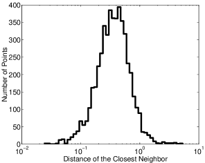
Figure 1: Distibution of the distances between each reconstructed vector and its closest neighbor for the dataset discussed in sec. III.

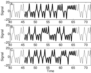
Figure 2: Panel A) shows portion of the time series discussed in sec. III. The blackened line was removed and the resulting gap was filled by applying the algorithm described in section II. The blackened lines in panels B) and C) are two different fillings.

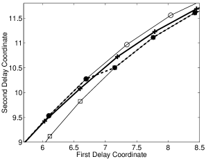
Figure 3: Plot of the first two components of the reconstructed vectors of: $\mathcal{M}_{1}$ (thick solid line with crosses); $\mathcal{L}_{1}$ (thick dashed line with asterisks); one orbit of $\mathcal{L}_{1}$ and its successors (thin line with open circles); the orbit consecutive to it and its predecessors (thin line with open squares). To illustrate the smoothing effect of minimizing functional (5), we only plot a very small portion of these sets in the vicinity of the jump between the consecutive orbits.

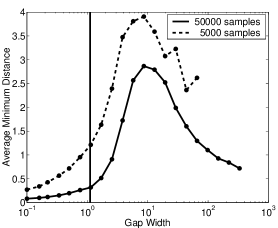
Figure 4: Average minimum distance of sinchronous points in the 1-jump forward and backward branch as a function of gap width. The dashed line refers to the dataset discussed in sec. III, the solid line refers to a ten times longer extension of that dataset. The vertical line marks the Lyapunov time $\lambda^{-1}\approx 1.1$.

References

- (1) F. Takens, in Dynamical Systems and Turbulence, R. Mañé, D. Rand, and L. S. Young (eds.), Warwick 1980, Lecture Notes in Math. (Springer, Berlin, 1981) , Vol. 898.
- (2) T. Sauer, J. A. Yorke, and M. Casdagli, J. Stat. Phys., 65, 579, (1991).
- (3) M. Casdagli, S. Eubank, J. D. Farmer, and J. Gibson, Physica D, 51, 52, (1991).
- (4) A. Provenzale, L.A. Smith, R. Vio, and G. Murante, Physica D, 58, 31, (1992).
- (5) J. Theiler, Phys. Rev. A, 34, 2427, (1986).
- (6) J. Froyland and K. H. Alfsen, Phys. Rev. A, 29, 2928, (1984).
- (7) M. Casdagli, Physica D, 35, 335, (1989).
- (8) J. D. Farmer and J. J. Sidorowich, Phys. Rev. Lett., 59, 845, (1987).
- (9) T. Serre, M. Auvergne, and M. J. Goupil, Astron. Astrophys., 259, 404, (1992).
- (10) E. N. Lorenz, J. Atmos. Sci., 20, 130, (1963).
- (11) W. H. Press, S. A. Teukolsky, W. T. Vetterling, and B. P. Flannery, Numerical Recipes in C: The Art of Scientific Computing, Cambridge University Press, Cambridge, (1992).
- (12) J.-P. Eckmann and D. Ruelle, 57, 617, (1985).
- (13) T. Erber, B. Schweizer, and A. Sklar, Commun. Math. Phys., 29, 311, (1973).
- (14) F. Paparella, A. Provenzale, L. A. Smith, C. Taricco, R. Vio, Phys. Lett. A, 235, 233, (1997).