Nonlinear dynamics and chaos in parametric sound generation

Nonlinear dynamics and chaos in parametric sound generation

Abstract

A theoretical analysis of the subharmonic generation process in an acoustical resonator (interferometer) with plane walls is performed. It is shown that, when both the pumping wave and the generated subharmonic are detuned with respect to the resonator modes, the fields can display complex temporal behaviour such as self-pulsing and chaos. A discussion about the acoustical parameters required for the experimental observation of the phenomenon is given.

I. INTRODUCTION.

Nonlinear dynamical phenomena have been reported in several acoustical systems. Different complex scenarios of temporal evolution, including self-pulsing, period doubling and deterministic chaos, are typically observed in a large variety of driven oscillators, such as nonlinear resonators, musical instruments or ultrasonic cavitation (for a review, see Ref. 1). In the particular resonator configuration, self-action of sound propagating in a viscid fliud, where the thermal mechanism of nonlinearity is dominant, has been studied theoretical and experimentally, and the onset of bistable, self-pulsed and chaotic regimes has been shown to occur with precedence to another acoustical nonlinear effects related to the elastic (quadratic) nonlinearity of the medium.Lyakhov93 These nonthermal effects, involving the appearance of new frequencies not present in the driving source, provoke the excitation of higher harmonics of the driving source (which in the absence of dispersion leads to waveform distortion and ultimately to the development of shock waves) or the frequency division of the input wave (subharmonics), an effect so called parametric sound generation. The latter phenomenon consist in the resonant interaction of a triad of waves with frequencies $\omega_{0},\omega_{1}$ and $\omega_{2}$, which are related by the energy conservation condition $\omega_{0}=\omega_{1}+\omega_{2}$. The process is initiated by an input pumping wave of frequency $\omega_{0}$ which, due to the propagation in the nonlinear medium, generates a pair of waves with frequencies $\omega_{1}$ and $\omega_{2}$. When the wave interaction occurs in a resonator, a threshold value for the input amplitude is required. This process has been described before by several authors under different conditions, either theoretical and experimentally.Korpel65 ; Adler70 ; Yen75 ; Ostrovsky76

It is important to note that the presence of higher harmonics can be avoided by different means. One method considers that the interaction takes place in a dispersive system. Dispersion allows that only few modes, those satisfying given synchronism conditions, participate in the interaction process. In finite geometries, such as waveguides Hamilton87 or resonators,Ostrovsky78 the dispersion is introduced by the lateral boundaries. Different resonance modes, propagating at different angles, propagate with different effective phase velocities. However, in homogeneous unbounded systems dispersion is usually not present. Different dispersion mechanisms have been proposed in nonlinear acoustics, such as propagation in bubbly or layered (periodic) media,Hamiltonbook which makes sound velocity propagation to be wavelength dependent. Other proposed mechanisms are, for example, media with selective absorption, in which selected spectral components experience strong losses and may be removed from the wave field.Zarembo74 , or resonators where the end walls present some frequency-dependent complex impedance.Yen75 In this case, the resonance modes of the resonator are not integrally related, and by proper adjustment of the resonator parameters one can get that only few modes, those lying close to a cavity resonance, reach a signifficant amplitude. Under this conditions, a spectral approach to the problem results appropriate, as has been proposed and experimentally confirmed in Ref. 6.

Therefore the selective effect of the resonator allows to reduce the study of parametric sound generation to the interaction of three field modes, correspondig to the driving (fundamental) and subharmonic frequencies, and to describe this interaction through a small set of nonlinear coupled differential equations. In the present work we describe the particular degenerate case of subharmonic generation, where $\omega_{1}=\omega_{2}$ and consequently $\omega_{0}=2\omega_{1},$ being $\omega_{0}$ the fundamental and $\omega_{1}$ generated subharmonic, both quasi-resonant with a corresponding resonance mode. This degenerate case has been the matter of previous experimental studies,Yen75 ; Ostrovsky78 and the observation of dynamical behaviour has been reported.Ostrovsky78 ; cook89 However, despite the experimental observation of complex temporal dynamics in this system, a theoretical framework supporting these effects and taking into account the peculiarities of the acoustic systems is absent. The main purpose of this work is to establish the necessary conditions for the development of nonlinear dynamics in an acoustic resonator where parametric generation of sound takes place.

II. MODEL EQUATIONS.

We consider a resonator with plane walls with finite width (acoustic interferometer) driven at a frequency $\omega_{0}$, and that the wave interaction is only effective among two resonant frequencies: the pump $\omega_{0}$ and the subharmonic $\omega_{1}$, for which the relation $\omega_{0}=2\omega_{1}$ hold. The field inside the resonator can then be expanded as

$$p(\mathbf{r},t)=\sum_{j=1}^{2}P_{j}(\mathbf{r},t),$$ (1)

where $P_{j}(\mathbf{r},t)$ are the wave components related with the frequency $\omega_{j}$. Restricting the analysis to a one-dimensional resonator, where quasi-plane waves propagate on the $z$ axis, and taking into account that, due to reflections in the walls, there exist waves propagating simultaneously in opposite directions, the wave components take the form

$$P_{j}(z,t)=p_{j}(t)\cos\left(k_{j}^{c}z\right)e^{-i\omega_{j}t}+c.c.,$$ (2)

where $k_{j}^{c}$ a cavity eigenmode.

Under the assumption of plane waves inside a resonator with highly reflecting ends (weak cavity losses), the model for the time evolution of degenerate parametric sound generation reads victorsm03

$$\frac{\partial p_{0}}{\partial t} =E-\gamma_{0}(1+i\Delta_{0})p_{0}-i\beta p_{1}^{2},$$

$$\frac{\partial p_{1}}{\partial t} =-\gamma_{1}(1+i\Delta_{1})p_{1}-i\beta p_{1}^{\star}p_{0},$$ (3)

where the variables $p_{i}\;(i=0,1)$ are the complex slow-varying amplitudes of the fundamental and subharmonic fields, with angular frequencies $\omega_{i}.$ The rest of parameters and their units are: the pump $E$ ($Pa/s$), proportional to the injected amplitude $p_{in}$ ($Pa$) of the fundamental mode and acting as a control parameter; the loss coefficient $\gamma_{i}$ ($s^{-1}$); the nonlinear coupling parameter $\beta$ ($s^{-1}Pa^{-1}$), and the adimensional detuning parameter $\Delta_{i}$, proportional to the frequency mistuning between the field frequency $\omega_{i}$ and the closest resonator eigenfrequencies $\omega_{i}^{c}$. All these parameters are defined as

$$E =\frac{c}{2L}\sqrt{\mathcal{T}_{0}}p_{in},$$

$$\gamma_{i} =\frac{c\mathcal{T}_{0}}{2L}+\kappa_{i},$$

$$\Delta_{i} =\frac{\omega_{i}^{c}-\omega_{i}}{\gamma i},$$ (4)

$$\beta =\frac{\varepsilon\omega_{1}}{4\rho_{0}c^{2}}.$$

being $c$ the propagation velocities, $\mathcal{T}_{i}\;$and $\mathcal{R}_{i},\$the transmission and reflection coefficients at resonator ends ($\mathcal{R}_{i}>>\mathcal{T}_{i}$ has been assumed), $L$ the length of the resonator, $\varepsilon\;$the nonlinearity parameter, $\rho_{0}$ the medium density and $\kappa_{i}=\delta k_{i}^{2}/2$ account for losses related to diffusivity of sound in the medium $\delta$. A detailed derivation of this model, generalized to include the field dependence on the transversal coordinates (not considered here for simplicity) can be found in Ref. 15. The same equations have been obtained in Ref. 3 for waveguide resonators (althought with different coupling coefficients, dependent on the structure of the interacting transverse modes), or for one-dimensional acoustic interferometers in Ref. 6, in a form identical to Eqs. (3).

The model (3) has been also derived in the context of nonlinear optics.Lugiato88 where the existence of complex temporal dynamics has been reported. In the next section we review the main results concerning the solutions and its stability properties for our particular acoustic system.

III. STATIONARY SOLUTIONS.

Two stationary solutions of (3) are obtained when the temporal derivatives vanish.Ostrovsky76 The simplest case corresponds to the trivial solution,

$$\overline{p}_{0}=\frac{E}{\gamma_{0}\left(1+i\Delta_{0}\right)},\,\overline{p}_{1}=0,$$ (5)

characterized by a null value of the subharmonic field inside the resonator. Increasing the pump value $E$ this solution bifurcates into a new solution, in which also the subharmonic field has a nonzero amplitude $\left|\overline{p}_{1}\right|$, given by

$$\left|\overline{p}_{1}\right|^{2} = \frac{1}{\beta^{2}}(\gamma_{0}\gamma_{1}(\Delta_{0}\Delta_{1}-1)\pm$$

$$\sqrt{\beta^{2}\left|E\right|^{2}-\gamma_{0}^{2}\gamma_{1}^{2}\left(\Delta_{0}+\Delta_{1}\right)^{2}}),$$

while the stationary fundamental amplitude $\left|\overline{p}_{0}\right|$ takes the value

$$\left|\overline{p}_{0}\right|=\frac{\gamma_{1}}{\beta}\sqrt{1+\Delta_{1}^{2}},$$ (7)

The emergence of this finite amplitude solution corresponds to the process of subharmonic generation. Note that the fundamental amplitude above the threshold is independent of the value of the injected pump, which means that all the energy is transferred to the subharmonic wave.

The transition from solutions (5) to (III. STATIONARY SOLUTIONS.) occurs at a critical pump amplitude

$$\left|E\right|=\frac{\gamma_{0}\gamma_{1}}{\beta}\sqrt{\left(1+\Delta_{0}^{2}\right)\left(1+\Delta_{1}^{2}\right)},$$ (8)

beyond which the trivial solution is unstable. These results have been confirmed experimentally in Ref. 3. The character of the bifurcation depends on the detuning values. As demonstrated in Ref. 3, and also in the optical context,Lugiato88 the bifurcation is supercritical when $\Delta_{0}\Delta_{1}<1$, and subcritical when $\Delta_{0}\Delta_{1}>1$. In the latter case, both trivial and finite amplitude solutions can coexist for given sets of the parameters, which results in a regime of bistability between different solutions. Figure 1 illustrates the form of the solutions in these two regimes.

Figure 1: Bifurcation diagram of the subharmonic field in the monostable (a) and bistable (b) cases. Subharmonic detuning values are $\Delta_{1}=2.4$ (a), and $\Delta_{1}=-2.4$ (b). The rest of parameters are $\Delta_{0}=1,$ $\beta=0.002$ and $\gamma_{0}=\gamma_{1}=500$ (see text below). Pressure units are given in $Pa$. Unstable branches are depicted in dashed lines, and the black square correspond to a Hopf bifurcation point.

IV. LINEAR STABILITY ANALYSIS.

In order to demonstrate the possibility of temporal dynamics in this system, the stability of the previous stationary solutions has been investigated by substituting in Eqs. (3) and their complex conjugate a perturbed solution in the form

$$p_{i}\left(t\right)=\overline{p}_{i}+\delta p_{i}(t)=\overline{p}_{i}+\overline{\delta p}_{i}\;e^{\lambda t},$$ (9)

where $\overline{p}_{i}$ are the particular stationary values. By linearizing the resulting equations around the small perturbations $\delta p_{i}$, one obtains $\lambda$ as the eigenvalues of the stability matrix that relates the vector of the perturbations $\left(\delta p_{i}(t),\delta p_{i}^{\ast}(t)\right)$ with their temporal derivatives. The instability of the solution is determined by the existence of positive real parts of the roots $\lambda$ of the characteristic polynomial,

$$\lambda^{4}+c_{1}\lambda^{3}+c_{2}\lambda^{2}+c_{3}\lambda+c_{4}=0$$ (10)

where, for the finite amplitude solution Eq. (III. STATIONARY SOLUTIONS.) and (7), the coefficients take the form

$$c_{1} =2\left(\gamma_{0}+\gamma_{1}\right),$$

$$c_{2} =4\beta^{2}\left|\overline{p}_{1}\right|^{2}+\gamma_{0}^{2}+4\gamma_{0}\gamma_{1}+\gamma_{0}\Delta_{0}^{2},$$

$$c_{3} =4\beta^{2}\left|\overline{p}_{1}\right|^{2}\left(\gamma_{0}+\gamma_{1}\right)+2\gamma_{0}^{2}\gamma_{1}\left(1+\Delta_{0}^{2}\right),$$

$$c_{4} =4\beta^{2}\left|\overline{p}_{1}\right|^{2}\left(\beta^{2}\left|\overline{p}_{1}\right|^{2}-\gamma_{0}\gamma_{1}\left(\Delta_{0}\Delta_{1}-1\right)\right).$$ (11)

Instead of solving the quartic polynomial Eq. (10) to find the eigenvalues, we apply the Hurwitz criterion (see e.g. Ref. 17), which states that the solution becomes unstable when at least one of the following conditions are violated:

$$c_{1}\eqslantgtr 0,\ c_{2}\eqslantgtr 0,\ c_{3}\eqslantgtr 0,\ c_{4}\eqslantgtr 0$$ (12a)

$$c_{1}c_{2}-c_{3}\eqslantgtr 0$$ (12b)

$$c_{3}\left(c_{1}c_{2}-c_{3}\right)-c_{1}^{2}c_{4}\eqslantgtr 0.$$ (12c)

Condition (12b) is always fulfilled. In conditions (12a), only $c_{4}\;$can become negative, corresponding with the turning point of the stationary solution of the $\Delta_{0}\Delta_{1}>1\;$case (see Fig. 1b). This means that the lower branch of the stationary solution, represented by the dashed line in Fig. 1 is always unstable.

Finally, the equality in condition (12c) denotes the existence of a pair of complex conjugate eigenvalues with vanishing real part ($\lambda=\pm i\omega$), which are indicative of a Hopf bifurcation which gives rise to oscillating solutions, with angular frequency $\omega$. Substituting (11) in (12c) the instability condition reads

$$\gamma_{0}^{2}\gamma_{1}\left(1+\Delta_{0}^{2}\right)\left(\left(\gamma_{0}+2\gamma_{1}\right)^{2}+\gamma_{0}^{2}\Delta_{0}^{2}\right)+$$ (13)

$$2\left(\gamma_{0}+\gamma_{1}\right)^{2}\left(\gamma_{0}\left(1+\Delta_{0}^{2}\right)+2\gamma_{1}\left(1+\Delta_{0}\Delta_{1}\right)\right)\beta^{2}\left|\overline{p}_{1}\right|^{2}\geqq 0.$$

which is fullfilled when the subharmonic amplitude reaches the value

$$\left|\overline{p}_{1}\right|_{HB}^{2}=\frac{-\gamma_{0}^{2}\gamma_{1}\left(1+\Delta_{0}^{2}\right)\left(\left(\gamma_{0}+2\gamma_{1}\right)^{2}+\gamma_{0}^{2}\Delta_{0}^{2}\right)}{2\beta^{2}\left(\gamma_{0}+\gamma_{1}\right)^{2}\left(\gamma_{0}\left(1+\Delta_{0}^{2}\right)+2\gamma_{1}\left(1+\Delta_{0}\Delta_{1}\right)\right)},$$ (14)

The positiveness of the threshold value (14) requires an additional condition, namely that the product of the detunings satisfies

$$\Delta_{0}\Delta_{1}<-\frac{1}{2\gamma_{1}}\left(\gamma_{0}+2\gamma_{1}+\gamma_{0}\Delta_{0}^{2}\right).$$ (15)

The latter condition excludes bistability (which requires $\Delta_{0}\Delta_{1}>1$). Consequently, condition (15) implies that the bifurcation that leads to subharmonic generation is always supercritical, and then only single-valued solutions can undergo a Hopf bifurcation (see Fig. 1). The angular frequency of the oscillations at the Hopf instability point can be found by substituting $\lambda=i\omega$ in (13), and reads

$$\omega_{HB}=\sqrt{2\beta^{2}\left|p_{1}\right|_{HB}^{2}+\frac{\gamma_{0}^{2}\gamma_{1}\left(1+\Delta_{0}^{2}\right)}{\gamma_{0}+\gamma_{1}}},$$ (16)

where $\left|p_{1}\right|_{HB}$ is the subharmonic amplitude at the Hopf bifurcation point given by Eq. (14).

V. ACOUSTICAL ESTIMATES.

For a better understanding of the predictions of the model and to assure their experimental validity, a special care must be taken when choosing the acoustical parameters involved in the theory. We will first refer such quantities to the experimental investigation of subharmonic generation in an acoustic interferometer described in detail by Yen Yen75 . It consists in a three sectioned resonator (quartz crystal$\mathcal{-}$water$\mathcal{-}$quartz crystal) of variable length, operated at 26^∘C. Our aim is to evaluate the threshold for subharmonic generation Eq. (8) and the possibility of its destabilization at the value given by (14). From Ref. 6 we obtain realistic acoustical values for the field decay rates $\gamma_{i}$, the detunings $\Delta_{i}$ and the nonlinearity parameter $\beta$ involved in the model. These parameters depend, as defined in (4), on sound frequencies and velocities, medium nonlinearity $\varepsilon$, cavity length and reflectivity of boundaries, and the eigenfrequencies of the resonator. In Ref. 6 the resonance modes of the one-dimensional resonator were calculated by using the formula

$$R\left(\tan k_{w}^{\prime}D+\tan k_{w}^{\prime}H\right)+\tan k^{\prime}S-$$ (17)

$$R^{2}\tan k_{w}^{\prime}D\tan k_{w}^{\prime}H\tan k^{\prime}S=0$$

where $R$ is the ratio of wall impedance to medium impedance, $k^{\prime}$ and $k_{w}^{\prime}$ are the wavenumbers in the fluid and the walls respectively, and $D,H$ and $S$ are the thicknesess of the two end walls and the length of the actual resonator, respectively. From (17) results an non-equidistant spectrum, which is required to allow the fulfillment of the condition (15). In the case of an equidistant spectrum (corresponding to a perfect resonator without losses), the detunings are obeyed to have the same sign.

The values of these resonance modes, as well as the quality factor $Q_{i}$ associated with them, were also experimentally measured in Ref. 6. The pumping frequency was about 1.6 MHz, for which a subharmonic emission of 0.8 MHz is expected. The closest resonator eigenfrequencies to such fundamental and subharmonic emissions were $f_{0}^{c}=1.5853$ MHz and $f_{1}^{c}=0.8088$ MHz, with associated quality factors of 4700 and 2600, respectively. The quality factor allows to estimate directly the decay rates $\gamma_{i}$ using the relation $Q_{i}=\omega_{i}/2\gamma_{i}$, and the corresponding detuning is calculated then from (4). The nonlinear coupling parameter $\beta$ defined in Eq. (4) is determined by the subharmonic frequency $\omega_{1},$ the medium nonlinearity ($\varepsilon=3.5$ for water), and the sound velocity $c=1500\$m/s. Note that the possible values of the detunings $\Delta_{0}$ and $\Delta_{1}$ are restricted by the non-equidistant eigenfrequencies of the resonator and the parametric character of the process, since $\omega_{0}=2\omega_{1}$.

The threshold of subharmonic generation was also measured by Yen,Yen75 and given in terms of the fundamental pressure amplitude inside the resonator at the bifurcation point given by Eq. (7). The model predicts its dependence on the subharmonic field detuning and on the subharmonic frequency through the coupling parameter $\beta$. The lowest theoretical value of the threshold corresponds to a perfect tuning of the subharmonic field with a cavity eigenmode, that is for a fixed $f_{1}=0.8088$ MHz and the corresponding fundamental $f_{0}=1.6176$ MHz, results $\Delta_{1}=0,$ and $\Delta_{0}=-187.7$, and nonlinear coupling parameter $\beta=0.002$ $s^{-1}Pa^{-1}$. The predicted fundamental pressure amplitude at threshold is therefore about $\left|p_{0}\right|=0.49$ MPa or $4.9$ bar. The lowest threshold reported in Ref. 6 is about $8.8$ bar, measured for a frequency close to the cavity mode $f_{0}^{c}=1.5853$ MHz. This difference can be due to the finite bandwidth of the exciting transducer in opposition to the monochromatic pump considered here, since the introduction of small detunings on the expected subharmonic field causes a sensitive and rapid increase of the subharmonic emission threshold.

After the switching-on of the subharmonic field the system supports constant pressure amplitudes of both fundamental and subharmonic fields, corresponding to the solutions (III. STATIONARY SOLUTIONS.) and (7). In order to observe self-oscillations of the amplitudes, the Hopf bifurcation condition (15) must be fulfilled, e.g. by increasing the detuning of the subharmonic field. One would get this by tuning the frequency of the subharmonic up to the value $f_{1}=0.8072\;$MHz, for which $\Delta_{1}=52.4551$ and $\Delta_{0}=-94.7686$. Unfortunately, when trying to achieve the detunings condition for instabilities, the subharmonic emission threshold grows up to the unrealistic value $\left|\overline{p}_{0}\right|=26$ MPa. For the same parameters, the Hopf bifurcation threshold is obtained for a subharmonic amplitude of $\left|\overline{p}_{1HB}\right|=1.14$ GPa. Clearly, for this particular resonator mode distribution the operation regime should be always in the steady state with constant pressure amplitudes. This could be the reason why dynamical states have not been described neither in Ref. 6 nor in other experimental works in which the conditions were probably similar.

Nevertheless the destabilisation of the subharmonic regime would explain certain phenomena previously described in the literature, such as self-modulation of the fields Ostrovsky78 or possible chaotic behaviour cook89 . We estimate next the necessary conditions for the occurrence of these phenomena at reasonable values. The resonator described in Ref. 11 corresponds to that described above; two air backed quartz transducers placed in a Fabry-Perot configuration with water, with a regulable separation between 5 and 10 cm. The driven transducer had a resonant frequency $f_{0}=$ $1$ MHz and the other had a lower resonance frequency. We take this frequency as the fundamental for our estimations and evaluate the remaining parameters of the desired resonator. From inspection of Eq. (8) it follows that the subharmonic emission threshold can be lowered by improving the quality of the resonator for both modes. However, the behaviour of the second threshold it is not so evident: Fig. 2 shows the dependence of the pressure amplitude of the subharmonic field at the Hopf bifurcation on the ratio of the quality factors affecting to both fundamental and subharmonic fields. It evidences that instabilities are reached earlier when the fundamental field has significant lower losses than the corresponding subharmonic. According to this, we set $Q_{0}=6000$ and $Q_{1}=3000,$ which are realistic values if compared to those measured in Ref. 6.

Figure 2: Dependence of the pressure amplitude of the subharmonic field at the Hopf bifurcation ($\left|\overline{p}_{1}\right|_{HB}$) on the ratio of the quality factors of fundamental and subharmonic fields. The parameters are $\Delta_{0}=1,\Delta_{1}=-2.4,\beta=0.002$ and $Q_{1}=3000.$ The value of $Q_{0}$ is kept free.

The resonator must meet another important restriction concerning its frequency distribution, in order to satisfy Eq. (15). In Fig. 3 are shown the combination of detunings that accomplish this condition for the given quality factors. The shadowed area represent detuning values which are compatible with the Hopf bifurcation condition (the inverted symmetrical figure, with opposite signs of both detunings, is also valid). One must also consider the lowest possible detunings in order to achieve the minimal value for the pressure amplitudes in both thresholds. Note that, whilst $\Delta_{0}$ can be arbitrarily small, the absolute value of $\Delta_{1}$ must be greater than $2$. A combination of values that reduce the thresholds to common experimental levels is $(\Delta_{0},\Delta_{1})=(1.0,-2.4)$, corresponding to an intracavity pressure amplitude of the fundamental mode at the first threshold of $\left|\overline{p}_{0}\right|=1.11$ MPa, and a subharmonic amplitude pressure at the Hopf bifurcation point of $\left|\overline{p}_{1HB}\right|=0.758\$MPa. From this discussion it follows that, in order to obtain experimentally the destabilisation of the subharmonic field, the resonator must be designed with a mode distribution that allows such values of detunings.

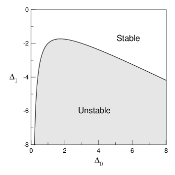
Figure 3: Detuning combinations required to fulfil the Hopf bifurcation condition.

The linear stability analysis can not predict the behaviour of the fields beyond the bifurcation points, and also does not give information about the subcritical or supercritical character of the bifurcation. In the next section we perform the numerical integration of the model (3) using the parameters estimated above.

VI. NUMERICAL SIMULATIONS.

Equations (3) have been numerically integrated by means of a fourth-order Runge-Kutta algorithm, and using the acoustical parameters discussed in the previous section. According to this, we have chosen the numerical values $\Delta_{0}=1,$ $\Delta_{1}=-2.4,$ $\gamma_{0}=\gamma_{1}=523.6$ ($s^{-1}$) and $\beta=0.0012$ ($s^{-1}Pa^{-1}$). As the control parameter we consider now the physical variable of the pump amplitude incident on the resonator $\left|p_{in}\right|$, related to the pump value $\left|E\right|$ appearing in the Eqs. (3) as $\left|p_{in}\right|=(2L/c)\sqrt{1/\mathcal{T}}$ $\left|E\right|$. The resonator has a length of $L=10$ cm, and the end walls a reflectivity coefficient $\mathcal{R}=0.9$, which is in agreement with the decay rate values considered above.

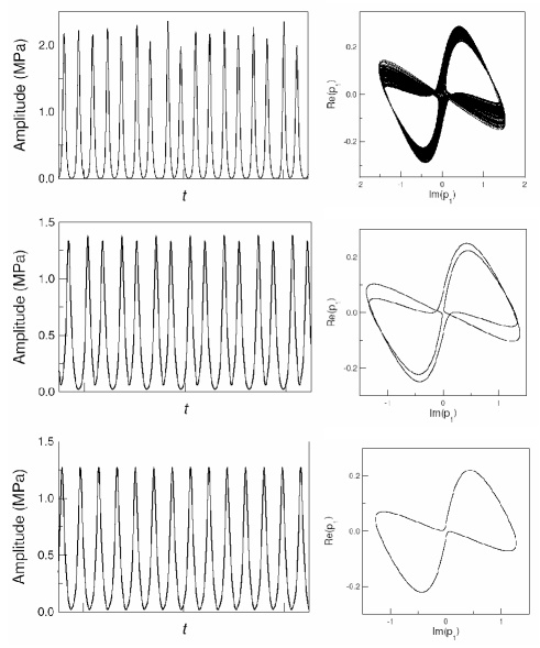
Figure 4: Time evolution (left) and phase portrait (right) of the sunharmonic field for $\Delta_{0}=1,\Delta_{1}=-2.4,\beta=0.0012,$ $\gamma_{0}=\gamma_{1}=523.6,$ and different drivings. (a) $\left|p_{in}\right|=0.60$ MPa. (b) $\left|p_{in}\right|=0.58$ MPa. (c) $\left|p_{in}\right|=0.55$ MPa.

The numerical results are summarized in Fig. 4. The show the existence of a bifurcation of the subharmonic solution Eq. (III. STATIONARY SOLUTIONS.) at the injected amplitude $\left|p_{in}\right|=0.60$ MPa, as predicted by the linear stability analysis. However, the temporal evolution of the fields near the bifurcation point is not oscillatory but chaotic, as shown in Fig. 4(a). At the right, the corresponding phase portrait is shown, where the dense structure of the attractor is appreciated, as corresponds to chaotic behaviour. When decreasing the injected amplitude below the bifurcation point, the temporal behaviour persists, denoting that the Hopf instability is subcritical. As pumping is decreased , the temporal evolution of the amplitude follows one of the universal scenarios leading to chaos, namely a period-doubling scenario or Feigenbaum route to chaos. Since we are decreasing the control parameter, we observe the transition from chaos to periodicity in an inverted way. Slightly below the bifurcation point, regular oscillations are observed with period eight ($P_{8}$) and period four ($P_{4}$), which exist in a narrow window. At $\left|p_{in}\right|=0.58$ MPa, the evolution is bi-periodic ($P_{2}$) as shown in Fig. 4(b). For $\left|p_{in}\right|=0.55$ MPa the evolution is periodic with a single period ($P_{1}$). This case is represented in Fig. 4(c). Further decreasing the control parameter, the system again enters in a chaotic regime, mediated a reversed period doubling cascade. This chaotic regime exist only in a narrow window, and the scenario reported above repeats until the value $\left|p_{in}\right|=0.53$ MPa, where the subharmonic field jumps again to the stable stationary branch given by Eqs. (III. STATIONARY SOLUTIONS.). This corresponds to the turning point of the dynamic branch, associated to a fold or saddle node bifurcation.

The complete scenario of bifurcations can be represented in a single plot (Fig. 5), where the frequency spectrum of solutions is given as a function of the control parameter. The subcritical character of the bifurcation, and the complexity of the temporal evolution in this system is evident here. Several chaotic windows are observed (dark horizontal bands, corresponding to a dense spectrum), always followed by a period-doubling sequence where $P_{8}$, $P_{4}$, $P_{2}$ and $P_{1}$ states are observed. In the plot a grey scale has been used, representing pressure leves ranging from 0 to 100 dB.

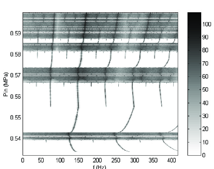
Figure 5: Spectrum of solutions as a function of the injected pump amplitude, for the parameters given in Fig. 4.

VII. CONCLUSIONS.

In this paper, the problem of subharmonic generation in a nonlinear acoustic resonator is treated from the point of view of nonlinear dynamics. A linear stability analysis reveals the possibility of time dependent solutions, which depending on parameters can be regular or chaotic. Numerical analysis are consistent with the theoretical predictions.

Althought the proposed model presents many analogies with similar systems studied in nonlinear optics, such as the two-level laser or the optical parametric oscillator, the peculiarities of acoustical resonators (specially the non-equidistant mode distribution, and the loss mechanisms) motivates a careful analysis. We conclude that the observability of the phenomena is fundamentally restricted by existence of low (experimentally achievable) threshold values, a situation which strongly depends on the resonator linear properties, such as mode distribution and quality factors. We believe that the proposed model could explain some experimental observations of complex dynamical behaviour in acoustic resonators reported in the past cook89 .

VIII. ACKNOWLEDGEMENTS

The authors thank Dr. H. Hobaek and Dr. Y.N. Makov for interesting discussions on the subject. The work was financially supported by the CICYT of the Spanish Government, under the project BFM2002-04369-C04-04.

References

- (1) W. Lauterborn, ”Nonlinear dynamics in acoustics”, Acustica 82, Suppl. 1 (1996).
- (2) G. A. Lyakhov, A. K. Proskuryakov, O. V. Umnova and K. F. Shipilov, ”Nonlinear oscillations regimes in an acoustic resonator”, Acoust. Phys. 39 (2), Mar.-Apr. (1993).
- (3) L.A. Ostrovsky and I.A. Soustova, “Theory of parametric sound generators”, Sov. Phys. Acoust. 22, 416 (1976).
- (4) A. Korpel and R. Adler, “Parametric phenomena observed on ultrasonic waves in water”, Appl. Phys. Lett. 7, 106 (1965).
- (5) L. Adler and M.A. Breazeale, J. Acoust. Soc. Am. 48, 1077 (1970).
- (6) N.Yen, “Experimental investigation of subharmonic generation in an acoustic interferometer”, J. Acoust. Soc. Am. 57, 1357 (1975).
- (7) M.F. Hamilton and J.A. TenCate, “Sum and difference frequency generation due to noncollinear wave interaction in a rectangular duct”, J. Acoust. Soc. Am. 81, 1703 (1987).
- (8) L.A. Ostrovsky, I.A. Soustova and A.M. Sutin, “Nonlinear and parametric phenomena in dispersive acoustic systems”, Acustica 39, 298 (1978).
- (9) M.F. Hamilton and D. Blackstock, Nonlinear Acoustics, Academic Press (1997)
- (10) L.K. Zarembo and O.Y. Serdoboloskaya, “To the problem of parametric amplification and parametric generation of acoustic waves”, Akust. Zh. 20, 726 (1974).
- (11) Bill D. Cook, ”Possible observation of chaos in acoustics” J. Acoust. Soc. Am. 85 S1, S5-S6 (1989).
- (12) V.J. Sánchez-Morcillo, ”Spontaneuos pattern formation in an acoustical resonator” J. Acoust. Soc. Am. 115, 111-119 (2004).
- (13) L.A. Lugiato, C. Oldano, C. Fabre, E. Giacobino and R.J. Horowicz, “Bistability, self-pulsing and chaos in optical parametric oscillators”, Nouvo Cimento 10D, 959-976 (1988).
- (14) H. Haken, Synergetics, 3rd edition, Springer-Verlag, Berlin (1983)