Localized patterns and hole solutions in one-dimension extended sytem

Abstract

The existence, stability properties, and bifurcation diagrams of localized patterns and hole solutions in one-dimensional extended systems is studied from the point of view of front interactions. An adequate envelope equation is derived from a prototype model that exhibits these particle-type solutions. This equation allow us to obtain an analytical expression for the front interaction, which is in good agreement with numerical simulations.

Non-equilibrium processes often lead in nature to the formation of spatial periodic structures developed from a homogeneous state through the spontaneous breaking of symmetries present in the system [1, 2]. In the last decade localized patterns or localized structures have been observed in different experiments: liquid crystals [3], gas discharge systems [4], chemical reactions [5], fluids [6], granular media [7], and nonlinear optics [8, 9]. One can understand these localized patterns as patterns extend only over a small portion of the spatial homogeneous systems. From the dynamic point of view, localized patterns in one-dimensional spatial systems are the homoclinic connection for the stationary dynamical system. Recently, from a geometrical point of view, the existence, stability properties, and bifurcation diagrams of localized patterns in one-dimensional extended systems have been studied [10].

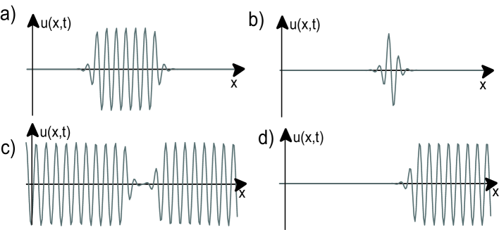
Figure 1: Particle type solutions appear in the subcritical Swift-Hohenberg equation. The parameters have been chosen as $\epsilon=-0.16$, $\nu=1.00$, and $q=0.70$. (a) Localized pattern, (b) shortest localized pattern, (c) hole solution and (d) front solution.

The aim of this manuscript is to describe how one-dimensional localized patterns and hole solutions arise from front interactions. From a prototype model that exhibits localized patterns and hole solutions, the subcritical Swift-Hohenberg equation, we deduce an adequate equation for the envelope of these particle type solutions. This model has a front solution that connects a stable homogeneous state with an also stable but spatially periodic one. Due to the oscillatory nature of the front interaction, which alternates between attractive and repulsive, we can infer the existence, stability properties, and bifurcation diagrams of localized patterns and hole solutions. Hence, we reobtain the bifurcation diagrams of localized patterns and hole solution deduced from horseshoe behavior of the attractive and repulsive manifold of ordinary differential equations [10].

Lets consider a prototype model that exhibits localized patterns and hole solutions in one-dimension extended system, the subcritical Swift-Hohenberg equation [11]:

$$\partial_{t}u=\varepsilon u+\nu u^{3}-u^{5}-(\partial_{xx}+q^{2})^{2}u,$$ (1)

where $u\left(x,t\right)$ is an order parameter, $\varepsilon-q^{4}$ is the bifurcation parameter, $q$ is the wave-number of periodic spatial solutions, and $\nu$ is the control parameter of the type of bifurcation, supercritical or subcritical. This model describes the confluence of a stationary and an spatial subcritical bifurcation, when the parameters scale as $u\sim\varepsilon^{1/4}$, $\nu\sim\varepsilon^{1/2}$, $q\sim\varepsilon^{1/4}$, $\partial_{t}\sim\varepsilon$ and $\partial_{x}\sim\varepsilon^{1/4}$ ($\varepsilon\ll 1$). It is often employed in the description of patterns observed in Rayleigh-Benard convection and pattern forming systems [2]. In Fig. 1 we show typical localized patterns, hole solutions, and motionless front solutions obtained by this model. For small and negative $\nu$, and $9\nu^{2}/40<\varepsilon<0$, the system exhibits coexistence between a stable homogenous state $u(x)=0$ and a periodic spatial one $u(x)=\sqrt{\nu}\left(\sqrt{2(1+\sqrt{1+40\varepsilon/9\nu})}\cos\left(qx\right)\right)+o(\nu^{5/2})$. In this parameter region, one finds a front between these two stable states (cf. Fig. 1). In order to describe the front, localized patterns and hole solutions, we introduce the ansatz

$$u=\sqrt{\frac{2\nu}{10}}\varepsilon^{1/4}\left\{A\left(y=\frac{3\sqrt{\left|\varepsilon\right|}}{2\sqrt{10q}}x,\tau=\frac{9\nu^{2}\left|\varepsilon\right|}{10}t\right)+w_{1}\left(x,y,\tau\right)\right\}e^{iqx}+c.c,$$ (2)

where $A(y,\tau)$ is the envelope of the front solution, $w_{1}\left(x,y,\tau\right)$ is a small correction function of order $\varepsilon$, and $\left\{y,\tau\right\}$ are slow variables. Note that in this ansatz we consider that $q$ is order one, or larger that the other parameters. Introducing the above ansatz in Eq. (1) and linearizing in $w_{1}$, we find the following solvability condition

$$\partial_{\tau}A=\epsilon A+\left|A\right|^{2}A-\left|A\right|^{4}A+\partial_{yy}A+\left(\frac{A^{3}}{9\nu}-\frac{A^{3}\left|A\right|^{2}}{2}\right)e^{\frac{2iqy}{a\sqrt{\left|\varepsilon\right|}}}-\frac{A^{5}}{10}e^{\frac{4iqy}{a\sqrt{\left|\varepsilon\right|}}},$$ (3)

where $\epsilon\equiv 10\varepsilon/9\nu^{2}$, and $a\equiv 3\nu/2\sqrt{10}q$ . The terms proportional to the exponential are non-resonant, that is, one can eliminate these terms by an asymptotic change of variable. Furthermore, they have rapidly varying oscillations in the limit $\epsilon\rightarrow 0$. Hence, one usually neglects these terms. Note that, the above envelope equation is a universal model, close to a spatial bifurcation, of a system that exhibits coexistence between an homogeneous state and spatial periodic one. In general, one can use an ansatz similar to (2) and noticing that the envelope satisfies independently the symmetries $\left\{x\rightarrow-x,\text{ }A\rightarrow\bar{A}\right\}$, and $\left\{x\rightarrow x+x_{o}\text{, }A\rightarrow Ae^{iqx_{o}}\right\}$ one derives equation (3).

When one considers only the resonant terms, it is straightforward to show that the system has a front solution between two homogeneous states, $0$ and $\left(1+\sqrt{1+4\epsilon}\right)/2$, when $-1/4<\epsilon<0$. This front propagates from the global stable to the metastable one, and it is motionless when the Maxwell point is reached at $\epsilon_{M}=-3/16$, and it has the form

$$a_{\pm}(y)=\sqrt{\frac{3/4}{1+e^{\pm\sqrt{3/4}(y-y_{o})}}}e^{i\theta},$$

where $y_{o}$ is the front’s core position, and $\theta$ is an arbitrary phase.

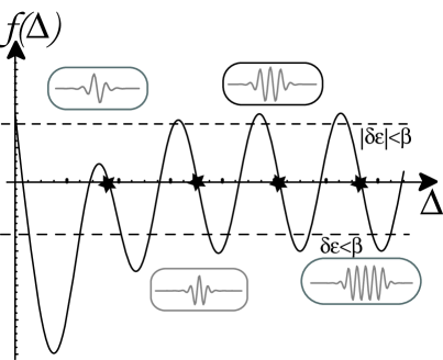
Figure 2: Oscillatory interaction force $f\left(\Delta\right)$. The inset figures are the stable localized patterns observed at the Maxwell point. The length of these localized patterns are represented by the stars. The dashed lines represent the effective abscissa that determine the size of localized patterns when $\varepsilon$ is changed.

To describe a localized pattern exhibited by (1) as a pair of two fronts, we must then consider the non-resonant terms in the envelope equation (3). We consider all these terms as perturbations because they have rapidly varying oscillations. Close to the Maxwell point, we use the ansatz

$$A_{LP}(y,\tau)=\left[a_{-}(y-y_{1}(\tau))+a_{+}(y-y_{2}(\tau))-\rho\left(y_{1},y_{2},y,\tau\right)\right]e^{i\theta\left(y_{1},y_{2},y,\tau\right)},$$

where $\left\{\rho,\theta\right\}$ are small correction functions, which are of order $\delta\epsilon\equiv(\epsilon-\epsilon_{M})$ and $y_{2}>y_{1}$. Introducing the above ansatz in equation (3), linearizing in $\left\{\rho,\theta\right\}$ and after straightforward calculations, we obtain the following solvability condition for the distance between the fronts

$$\frac{d\Delta}{d\tau}=f\left(\Delta\right)\equiv-\alpha\Delta\exp(-\sqrt{\frac{3}{4}}\Delta)+\beta\cos(2q\Delta/\sqrt{\epsilon})+2\delta\epsilon,$$ (4)

where $\Delta\equiv y_{2}-y_{1}$, $\alpha=27\sqrt{3}/64$ and $\beta=64\sqrt{3}q^{2}\exp(-q4\pi/\sqrt{\epsilon})/3\epsilon$. In Fig. 2, we display the interaction of the front pair. It is important to note that in one-dimensional extended systems, the dependence of the distance in the front interaction is only exponential [2]. The linear and periodic dependence of $\Delta$ is a consequence of the interaction (contained in the non-resonant terms) of the large scale with the small scale underlying the spatial periodic solution. The system has several equilibria, $f(\Delta^{\ast})=0$, and they are stable if $f^{\prime}\left(\Delta^{\ast}\right)<0$. Thus, the existence and stability of localized patterns is given by oscillatory nature of the interaction. As is illustrated in Fig. 2, the region of attractive and repulsive interaction is separated by localized patterns. Note that, the larger equilibria represent localized patterns with a bigger number of bumps. In order to understand the bifurcation diagrams of localized patterns, we consider the effect of change the bifurcation parameter $\epsilon$. Note that, modifying $\epsilon$ is equivalent to move the abscissa of the front interaction (cf. Fig. 2). First, we consider the case $\left|\delta\epsilon\right|>\beta$ and $\delta\epsilon<0$; the interaction is always attractive, that is, there is no equilibrium. Hence, if one takes into account a front that connects the homogenous state with spatial periodic state, then the spatial periodic state invades the homogenous one.

In Fig. 3, the thick solid line is the velocity of propagation of the front as function of the bifurcation parameter. Increasing $\epsilon$, one finds the first equilibrium point $\Delta=\infty$ for $\delta\epsilon=\delta\epsilon_{-}\equiv\beta$ and $\delta\epsilon<0$. Thus the system has a motionless front between the spatial periodic and homogenous states. Note that, this equilibrium point remains meanwhile $\left|\delta\epsilon\right|\leq\beta$, therefore this front is motionless in a parameter range. This phenomenon is well-known as Locking phenomenon and the interval $\left|\delta\epsilon\right|\leq\beta$ is denominated pining range [12]. For $\delta\epsilon>\beta$, the front propagates from the spatial periodic state to the homogenous one. Increasing $\delta\epsilon$ from $\delta\epsilon_{-},$ we observe that the equilibria, localized patterns, appear by saddle-node bifurcation and with length smaller than the previous ones, i.e., the localized patterns appear by pair, one stable and another unstable, and each time with less bumps. This sequence of bifurcations is illustrated in Fig. 3 by the points $c_{i}^{a}$. For $\delta\epsilon$ small, and close to the Maxwell point, the system has a family of infinite localized patterns. The length of the localized patterns are roughly multiple of that of the shortest localized state. Contrarily, for $\left|\delta\epsilon\right|>\beta$, the localized patterns disappear by saddle node bifurcation and increasing $\delta\epsilon$ the larger localized patterns disappear one after another. Hence, the shortest localized state is the last to disappear. In Fig. 3 are represent the sequence of these bifurcation by $c_{i}^{d}$.

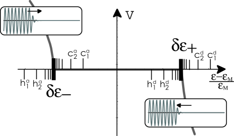
Figure 3: Speed of the front and bifurcation diagrams of the localized patterns and hole solutions as function of the bifurcation parameter. The thick solid line is the analytical formula of front speed. $c_{i}^{a}$ and $c_{i}^{d}$ ($h_{i}^{a}$ and $h_{i}^{d}$) represent the bifurcation points where the localized patterns with (hole solution without) i-bumps appears and disappear respectively.

The model (1) has different particle type solutions as: front solution, localized patterns and hole solutions. These solution are displayed in Fig. 1. From the front interaction the hole solution can be understood as the complement of localized patterns, because these solutions can be describe in term of the front as

$$A_{Hole}(y,\tau)=(a_{+}(y-y_{2}(\tau))+a_{-}(y-y_{2}(\tau))-\rho\left(y_{1},y_{2},y,\tau\right))e^{i\theta\left(y_{1},y_{2},y,\tau\right)},$$

where this solution asymptotically converges to a spatial periodic state. We obtain the same expression for the interaction (4) changing $\alpha$ by $-\alpha$. Therefore for these solutions, we obtain a similar bifurcation diagram of localized patterns but inverted, that is, the first hole in to appear and disappear by saddle-node bifurcation is the shortest hole, and successively the hole with shorter length appears one after the other and sequentially the solutions with shorter length disappear one after the other. In Fig. 3 is illustrated this sequence of bifurcations by $\left\{h_{i}^{a},h_{i}^{a}\right\}$. It is important to remark that the bifurcation diagram shown in Fig. 3 have been deduced from geometrical arguments based in horseshoe behavior of the attractive and repulsive manifold of a ordinary differential equation [10]. In the pining rage, the front solution is motionless. When one considers additive white noise, the noise induces front propagation [13]. The mean velocity of the front is zero only in the Maxwell point, that is, at the Maxwell point the front core describes a Brownian motion.

In conclusion, we have shown on the basis of the front interactions the existence, stability properties, and bifurcation diagrams of localized patterns and hole solutions in one-dimensional extended systems.

The simulation software DimX developed by P. Coullet and collaborators at the laboratory INLN in France has been used for all the numerical simulations. M.G.C. acknowledges the support of FONDECYT project 1051117, FONDAP grant 11980002, and ECOS-CONICYT collaboration programs.

References

- [1] G. Nicolis and I. Prigogine, Self-Organization in Non Equilibrium systems (J.Wiley & sons, New York, 1977).
- [2] M. Cross and P. Hohenberg, Rev. Modern Phys. 65, 581 (1993).
- [3] S. Pirkl, P. Ribire and P. Oswald, Liq. Cryst. 13 , 413 (1993).
- [4] Y.A Astrov and Y.A. Logvin, Phys. Rev. Lett. 79 , 2983 (1997).
- [5] K.L. Lee, W.D. McCormick, Q. Ouyang and H. Swinney, Science 261, 189 (1993).
- [6] O. Liobashevski, Y. Hamiwl, A. Agnon, Z. Reches and J. Fineberg, Phys. Rev. lett. 83, 3190 (1999).
- [7] Umbanhowar, F. Melo and H. Swinney, Nature 382, 793 (1996).
- [8] F.T. Arecchi, S. Boccaletti and P.L. Ramazza, Phys. Rep. 318,1 (1999).
- [9] B. Schapers, M. Feldmann, T. Ackemann and W. Lange, Phys. Rev. Lett. 85, 748 (2000).
- [10] P. Coullet, C. Riera and C. Tresser, Rev. Lett. 84, 3069 (2002).
- [11] H. Sakaguchi and H. Brand, Physica D 97, 274 (1996).
- [12] Y. Pomeau, Physica D 23, 3 (1986).
- [13] M.G. Clerc, C. Falcon and E. Tirapegui, submited to Phys. Rev. Lett.