An equation-free approach to coupled oscillator dynamics: the Kuramoto model example

Sung Joon Moon
Department of Chemical Engineering, Program in Applied and Computational Mathematics, Princeton University, Princeton, NJ 08544

Electronic mail address: moon@arnold.princeton.edu

Ioannis G. Kevrekidis
Department of Chemical Engineering, Program in Applied and Computational Mathematics; also Mathematics, Princeton University, Princeton, NJ 08544

Electronic mail address: yannis@princeton.edu

We present an equation-free multi-scale approach to the computational study of the collective dynamics of the Kuramoto model [Chemical Oscillations, Waves, and Turbulence, Springer-Verlag (1984)], a prototype model for coupled oscillator populations. Our study takes place in a reduced phase space of coarse-grained “observables” of the system: the first few moments of the oscillator phase angle distribution. We circumvent the derivation of explicit dynamical equations (approximately) governing the evolution of these coarse-grained macroscopic variables; instead we use the equation-free framework [Kevrekidis et al., Comm. Math. Sci. 1(4), 715 (2003)] to computationally solve these equations without obtaining them in closed form. In this approach, the numerical tasks for the conceptually existing but unavailable coarse-grained equations are implemented through short bursts of appropriately initialized simulations of the “fine-scale”, detailed coupled oscillator model. Coarse projective integration and coarse fixed point computations are illustrated.

1 Introduction

Coupled nonlinear oscillators can exhibit spontaneous emergence of order, a fundamental qualitative feature of many complex dynamical systems [Manrubia et al., 2004]. The collective, coarse-grained dynamics of coupled oscillator populations can provide insights in synchronization phenomena in many biological, chemical, and physical systems [Winfree, 1967; Walker, 1969; Buck, 1988; Gray et al., 1989; Ertl, 1991; Wiesenfeld et al., 1996; Néda et al., 2000; Oliva & Strogatz, 2001; Kiss et al., 2002]. In certain prototype models some exact results for the collective dynamics, mainly for an order parameter at the asymptotic states, can be obtained for either a few or an infinite number of oscillators (the so-called continuum limit) [Kuramoto, 1975; Kuramoto, 1984; Ariaratnam & Strogatz, 2001]; for instance, the continuum-limit Kuramoto model is well known to exhibit a phase transition at a critical coupling strength. However, general coupled oscillator models are seldom amenable to mathematical analysis, even for simple coupling topologies, and the understanding of the coarse-grained (emergent or macroscopic) dynamics of a given oscillator population remains limited. Even fundamental questions, such as global stability, spectral properties of the stationary solution, and finite-number fluctuations, often remain unanswered [Strogatz, 2000].

Understanding the coarse-grained behavior of dynamical systems consisting of a large number of mutually interacting entities is one of the main goals of statistical mechanics. In some cases, a fine-scale (or microscopic) model with a large number of degrees of freedom can be systematically reduced to a low-dimensional, coarse-grained model describing the dynamics by a small number of macroscopic variables (observables). However, such a reduction is rarely available in contemporary science or engineering dealing with specific complex systems. One often has to deal with a situation where a reliable model is available only at a fine-scale level (atomistic, individual-based), yet he/she is practically interested in the emergent, system level, coarse-grained dynamics. Even if a useful coarse-grained model is believed to exist at a practical closure level, explicit formulas for this model are often unavailable; the systematic derivation of closed formulas for such models is difficult without introducing many simplifying assumptions. In some cases, it is also possible that the description of a system simply does not close at a particular level of coarse-graining. In the case that a coarse-grained description exists, yet it is unavailable in closed form, the recently developed equation-free framework provides a systematic, computer-assisted approach to exploring coarse-grained macroscopic behavior without explicit knowledge of the coarse-grained equations themselves [Theodoropoulos et al., 2000; Gear et al., 2002; Kevrekidis et al., 2003; Kevrekidis et al., 2004]. This approach has been successfully combined with several classes of microscopic models, such as lattice-Boltzmann, kinetic Monte Carlo, and molecular dynamics simulators, to study the coarse-grained behavior of heterogeneous catalytic reactions, liquid crystal rheology, peptide fragment folding, etc. [Theodoropoulos et al., 2000; Gear et al., 2002; Makeev et al., 2002; Siettos et al., 2003, Hummer & Kevrekidis, 2003]. In this paper we illustrate the equation-free approach to the computational exploration of the coarse-grained dynamics of the Kuramoto model at the strong coupling limit.

The rest of the paper is organized as follows: The model under consideration and the regime in which we study it are described in Sec. 2. Some observations about the coarse-grained behavior and the equation-free analysis of phase-locked oscillator dynamics is presented in Sec. 3. Conceptually, the generalization of this approach for different oscillator models is straightforward; possible shortcomings and limitations will be addressed in Sec. 4, along with future research directions.

2 Background; the Kuramoto model

The Kuramoto model [Kuramoto, 1975] consists of $N$ equally weighted, all-to-all, phase-coupled limit-cycle oscillators, where each oscillator has its own natural frequency $\omega_{i}$ drawn from a prescribed distribution function $g(\omega)$. We choose $g(\omega)$ to be a Gaussian distribution of standard deviation 0.1; however, our analysis is not limited to this particular choice. The microscopic individual level dynamics is easily visualized by imagining oscillators as points running around on the unit circle. Due to rotational symmetry, the average frequency $\Omega=\sum_{i=1}^{N}\omega_{i}/N$ can be set to 0 without loss of generality; this corresponds to observing dynamics in the co-rotating frame at frequency $\Omega$. The governing equation for the $i$th oscillator phase angle $\theta_{i}$ is given by

$${d\theta_{i}\over dt}=\omega_{i}+{K\over N}\sum_{j=1}^{N}\sin(\theta_{j}-\theta_{i}),~{}~{}~{}1\leq i\leq N,$$ (1)

where $K\geq 0$ is the coupling strength; in this paper we arbitrarily set $N=300$ unless stated otherwise.

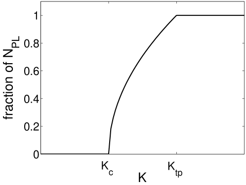
Figure 1: Qualitative schematic of the fraction of phase-locked oscillators in the Kuramoto model; there exist two critical values in K, the coupling strength. $N_{PL}$ is the number of phase-locked oscillators.

It is known that as $K$ is increased from 0 above some critical value $K_{c}$, more and more oscillators start to get synchronized (or phase-locked) until all the oscillators get fully synchronized at another critical value of $K_{tp}$ (Fig. 1). In our choice of $\Omega=0$, the fully synchronized state corresponds to an exact steady state of the “detailed”, fine-scale problem in the co-rotating frame. Such synchronization dynamics can be conveniently summarized by considering the fraction of the synchronized (phase-locked) oscillators as in Fig. 1, and conventionally described by a complex order parameter [Kuramoto, 1975]

$$re^{i\psi}={1\over N}\sum_{j=1}^{N}e^{i\theta_{j}},$$ (2)

where the radius $r$ measures the phase coherence, and $\psi$ is the average phase angle. Some exact results on the synchronization dynamics in the continuum-limit, in terms of this order parameter, are available [Kuramoto, 1984; Strogatz, 2000].

The transition from full to partial synchronization: We begin by restating certain facts about the nature of the second transition mentioned above, a transition between the full and the partial synchronization regime at $K=K_{tp}$, in the direction of decreasing $K$. A fully synchronized state (a “detailed” steady state) in the continuum limit corresponds to the solution to the following equations, the mean field type alternate form of Eq. (1) [Kuramoto, 1975]:

$${d\theta_{i}\over dt}=\Omega=\omega_{i}+rK\sin(\psi-\theta_{i}),~{}~{}~{}1\leq i\leq N,$$ (3)

where $\Omega$ is the common angular velocity of the fully synchronized oscillators (which is set to 0 in our case). It can be rewritten as

$${\Omega-\omega_{i}\over rK}=\sin(\psi-\theta_{i}),~{}~{}~{}1\leq i\leq N,$$ (4)

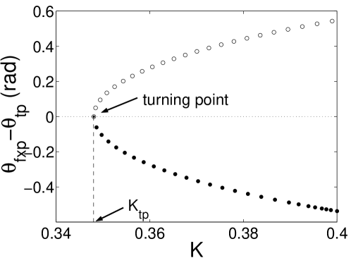
Figure 2: Bifurcation diagram of the oscillator that desynchronizes first with decreasing $K$ (this is the one with the maximum value of $|\omega_{i}-\left<\omega_{i}\right>|$, the “ extreme” oscillator). The transition from the full to the partial synchronization regime at $K=K_{tp}$ corresponds to a turning point of this oscillator phase angle at steady state ($\theta_{fxp}$), where $\theta_{tp}$ is the phase angle at the turning point. For the extreme oscillator, a saddle state and a stable node state collide in a saddle-node infinite period (sniper) bifurcation at $K=K_{tp}$.

where the absolute value of the right hand side (RHS) is bounded by unity. As $K$ approaches $K_{tp}$ from above, the LHS for the “extreme” oscillator (the oscillator in a particular family that has the maximum value of $|\Omega-\omega_{i}|$) first exceeds unity, and a real-valued solution to Eq. (4) ceases to exist. We obtain the detailed steady state solution to Eq. (1) as a function of $K$ for 300 oscillators by using AUTO2000 (see Ref. [37]), which is based on fixed point computation and pseudo-arclength continuation. The bifurcation diagram plotted in terms of the extreme oscillator phase angle reveals that the transition to the partially synchronized state corresponds to a turning point bifurcation, of the so-called saddle node infinite period, or “sniper” type (Fig. 2). Ermentrout and Kopell [Ermentrout and Kopell, 1984] have studied the transitions in the partial synchronization regime of a small number of oscillators, characterizing them as jumps in “frequency plateaus”.

Different random draws of $\omega_{i}$’s from $g(\omega)$ for a finite number of oscillators result in slightly different values of $K_{tp}$. We observe that $K_{tp}$ appears to follow a Gumbel type extreme distribution function [Kotz & Nadarajah, 2000], just as the maximum values of $|\Omega-\omega_{i}|$ do:

$$p(K_{tp})=\sigma^{-1}e^{-(K_{tp}-\mu)/\sigma}\exp[-e^{-(K_{tp}-\mu)/\sigma}],$$ (5)

where $\sigma$ and $\mu$ are parameters.

3 Coarse-grained dynamics of distribution moments

3.1 Observation

Our goal is to study the coarse-grained dynamics of an oscillator population, including the transient dynamics, in terms of coarse-grained observables. Since we are dealing with distributions, we naturally consider the first few moments as candidate coarse-grained variables (i.e. a kinetic theory-like description). The moments of a distribution are often easily accessible in practice, and have a clear physical meaning. We consider the dynamics of the moments of the phase angle distribution function $f(\theta)$,

$${\cal M}_{n}\equiv\left<\left(\theta-\left<\theta\right>\right)^{n}\right>={1\over N}\sum_{j=1}^{N}\left(\theta_{j}-{1\over N}\sum_{i=1}^{N}\theta_{i}\right)^{n},$$ (6)

where $n$ is a positive integer, and $\left<~{}\right>$ means an ensemble average. Since we choose to work with symmetric distributions, all the odd order moments are negligibly small. To obtain insights on the dynamics in this phase space, initial configurations of phase angles consistent with four sets of different values of the first two nonvanishing moments (${\cal M}_{2}$ and ${\cal M}_{4}$) are generated. These initial phase angle configurations do not have any statistical correlations with the natural frequencies of the oscillators to which they are assigned; this is an important issue to which we will return below. Evolution of such configurations, obtained by direct numerical integration of Eq. (1) reveals that the approach to a steady state consists of two stages. During the initial, relatively fast stage both moments decrease, and during a later slow stage the trajectory gradually approaches to an ultimate steady state along a common path, essentially a “slow manifold” of this dynamical system (Fig. 3). The phase angle distributions after the initial stage, when the one-dimensional slow manifold finally has been approached, are very close to Gaussian distributions (marked by the dotted line in Fig. 3). Once the trajectory approaches this slow manifold, the dynamics can be effectively described by (or observed on) any one even order moment.

In the following (Sec. 3.3), we will investigate the dynamics in the moment phase space following the equation-free approach [Theodoropoulos et al., 2000; Kevrekidis et al., 2003; Kevrekidis et al., 2004]; this should be contrasted with the conventional approach of first attempting to derive closed governing equations for the leading moments, and subsequently analyzing these equations.

3.2 Equation-free, coarse-grained multi-scale approach

The basic idea of the equation-free approach is to utilize fine-scale simulation as an experiment, in the form of a time-stepper: short bursts of appropriately initialized fine-scale simulations are used to estimate quantities relevant for scientific computation with the coarse-grained model. Function evaluations or derivative evaluations for the coarse variables involved in numerical tasks are thus substituted with estimation of these quantities, based on appropriately designed computational experiments with the detailed model. As a result, traditional continuum numerical techniques are directly “wrapped” around the fine-scale simulator. The essential steps can be summarized as follows:

• Identify a set of coarse-grained variables (observables) that sufficiently describe the system dynamics. We expect that a practically useful model exists and closes at the level of these coarse observables. In our analysis, we choose them to be the first two nonvanishing moments of the phase angle distributions, ${\cal M}_{2}$ and ${\cal M}_{4}$. We will denote the microscopic description by u ($\omega$’s and $\theta$’s in our case) and the macroscopic description by U (${\cal M}_{i}$’s).

• Choose an appropriate $lifting$ operator, $\mu$, which maps the macroscopic description U to one or more consistent microscopic descriptions u; note that this mapping is not uniquely defined. This operator constructs one or more fine-scale realizations of the problem consistent with the prescribed values of the coarse observables U (u = $\mu$U).

• Using a lifted, fine-scale realization as a new initial condition ${\bf u}(t_{0})$, run the microscopic simulator to obtain the values u($t_{0}+\Delta T$) at a later time ($\Delta T>0$). This procedure may be repeated for many different realizations ${\bf u}_{i}(t_{0})$ consistent with the same macroscopic initial condition ${\bf U}(t_{0})$, for purposes of ensemble averaging and variance reduction.

• Use an appropriate restriction operator $M$ which maps the microscopic description to the macroscopic description ${\bf U}(t)=M\left({\bf u}\left(t\right)\right)$. In our problem the restriction operator consists of simple evaluation of (ensemble averages of) the first two nonvanishing moments of the phase angle distribution, following their definitions in Eq. (6).

The above procedure results in the coarse timestepper $\Phi_{\Delta T}$:

$${\bf U}(t_{0}+\Delta T)\equiv\Phi_{\Delta T}({\bf U}(t_{0}))=M({\bf u}(t_{0}+\Delta T)),$$ (7)

a map from coarse variables at time $t=t_{0}$ to coarse variables at a later time $t=t_{0}+\Delta T$, constructed through the microscopic simulation. Given such information, obtained for a number of appropriately chosen coarse initial conditions, it is possible to implement many scientific computing algorithms to solve the unavailable coarse-grained equations; see Sec. 3.3 for details of such computations using two different methods. An important element of these algorithms is the fact that they function as protocols for the design of experiments with the fine-scale simulator: in the process of their execution they suggest new computational experiments with the coarse timestepper, and “bootstrap” their output toward the ultimate desired result. The success of this approach relies (as most of traditional continuum numerical analysis) on smoothness of the dynamics with respect to the coarse variables of interest (in time, in space and in phase space) and on the identification of proper lifting and restriction operators. An extensive discussion of this method can be found in [Kevrekidis et al., 2003].

During the lifting step, we create phase angle distributions conditioned on a finite number of prescribed moments. This is accomplished as follows: Given $g(\omega)$, phase angles consistent with different values of the moments are generated by drawing random values from the inverse cumulative distribution of the following distribution function

$$f_{I}(\theta)=f_{g}(\theta^{2})\left[1+\sum_{p=2}^{n(>2)}a_{p}S_{p}(\theta^{2})\right],$$ (8)

of which residual deviation from the Gaussian is expanded using Sonine polynomials (associated Laguerre polynomials) [Chapman, 1970] as basis functions; $f_{g}(\theta^{2})$ is a Gaussian distribution function with a prescribed value of ${\cal M}_{2}$, and $a_{p}$ is the coefficient of the $p$th order Sonine polynomial $S_{p}$. The value of ${\cal M}_{2p}$ is determined only by $a_{p}$, because the Sonine polynomials are otrhogonal with the Gaussian as the weighting function:

$$\int_{0}^{\infty}e^{-\theta^{2}}S_{p}(\theta^{2})S_{q}(\theta^{2})d\theta=\delta_{pq}{\cal N}_{p},$$ (9)

where $\theta$ is generally a $d$-dimensional vector, $\delta_{pq}$ is the Kronecker delta, and ${\cal N}_{p}$ is a normalization constant. The first three Sonine polynomials are given by $S_{0}(\theta^{2})=1$, $S_{1}(\theta^{2})={1\over 2}d-\theta^{2}$, and $S_{2}(\theta^{2})={1\over 8}d(d+2)-{1\over 2}(d+2)\theta^{2}+{1\over 2}\theta^{4}$, where $d$ is the dimension, which in our case is unity. Our lifting operator takes us from the values of a few lower order moments to the values of an equal number of Sonine polynomial coefficients, and then to a consistent phase angle distribution through $f_{I}(\theta)$. We consider only even functions for $f_{I}(\theta)$, due to the symmetry of $f(\theta)$ with our choice of $g(\omega)$.

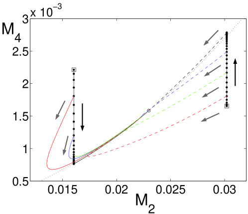
Figure 4: (Color) Two different random initializations of oscillators (marked by squares) are directly guided (shown by dot-dashed black lines) to the slow manifold by solving Eq. (1) along with a constraint on ${\cal M}_{2}$ for $K=0.7$. Each dot is separated in time by 0.1. Poor lifting results from relaxing the constraint before the slow manifold is approached (colored lines, constraint lifted at various times $t=$ 0.5, 1, 1.5, and 6 for red, blue, green, and black line, respectively). Arrows indicate the direction of increasing time.

One can clearly see in Fig. 3 that observation of the full system in the ${\cal M}_{2}-{\cal M}_{4}$ phase space gives trajectories crossing one another; this suggests that a deterministic description closing with only these two variables is not possible. However, once the initial fast evolution stage has run its course, trajectories evolve on an apparently one-dimensional slow manifold, which suggests that the long-time coarse-grained dynamics could be described in terms of a single observable, say ${\cal M}_{2}$ (or equivalently any other nonvanishing order moment). In other words, after sufficient time has elapsed, all the higher moments become slaved to ${\cal M}_{2}$. Considering this observation, a more successful lifting operator may be constructed from the following two steps, when ${\cal M}_{2}$ is chosen to be a coarse variable of interest: (1) Drawing phase angles from an $f_{I}(\theta)$ satisfying a desired value ${\cal M}_{2}=C_{1}$, and (2) numerically integrating Eq. (1) together with an algebraic constraint ${\cal M}_{2}-C_{1}=0$ until the trajectory approaches the slow manifold. After this preparatory computation, the lifting step is complete; the constraint is then removed, and the system is allowed to evolve in order to evaluate its coarse timestepper. This lifting operation results in an augmented problem (ODEs with an algebraic constraint) that is described by a system of differential algebraic equations (DAEs) of index 1. For our illustrative example, it is straightforward to solve this set of DAEs by using the Lagrange multiplier method and the package DASSL (see Ref. [38]). Direct integration of DAEs showing the relatively fast direct approach to the “mature” phase angle distributions on the slow manifold can be seen in Fig. 4. Once the constrained trajectory approaches the slow manifold, the constraint is relaxed, and we can observe its subsequent approach to the steady state along the manifold.

3.3 Equation-free computational results

We now compute the steady state values of the moments in the fully synchronized regime ($K>K_{tp}$) using two different continuum numerical methods in the equation-free framework: coarse projective integration and coarse fixed point computation.

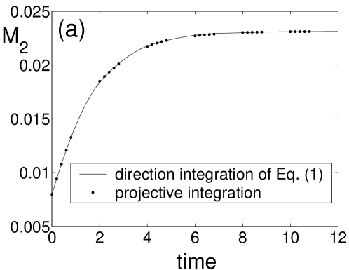
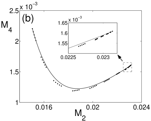
Figure 5: Transient approach to the steady state ($K=0.7$) computed through coarse projective integration (shown as dots), taking (a) only ${\cal M}_{2}$, and (b) both ${\cal M}_{2}$ and ${\cal M}_{4}$ as coarse variable(s). Full, fine scale integration is shown for comparison (solid line). In the projective integration computation, Eq. (1) is integrated only for the time intervals marked by dots, and the system is restricted to ${\cal M}_{2}$ (and ${\cal M}_{4}$) at uniformly distributed times (five dots in each group). The last three points are used to estimate the future value(s); lifting is then performed again, and the procedure repeated. For each lifting step, the same $g(\omega)$ was used. The inset in (b) shows the blow up near the steady state, where larger projection time steps are used for faster convergence.

We first evolve the system toward the stable steady state value of ${\cal M}_{2}$ using coarse projective integration [Gear & Kevrekidis, 2003a; 2003b]. The main assumption is that a macroscopic equation exists and closes in terms of ${\cal M}_{2}$; our observations of the long-term dynamics are consistent with such an assumption. Starting from a relatively short time ($\Delta t=0.8$) of direct integration, restriction of the results [shown as first group of five dots in Fig. 5 (a)] is used to estimate the coarse variable time derivative. Smoothness of the trajectory in time (Taylor series, as they appear in the simplest numerical integration schemes, such as forward Euler) is then used to “project” the value of the observable ${\cal M}_{2}$ in forward time. We then lift with this estimated value [shown as the fist dot in the next group in Fig. 5 (a)], and the whole procedure is repeated until the steady state is approached. During the evolution step, we do solve the full system of ODEs; but we do not solve it for all time: short bursts of detailed simulation are used to “jump” (and thus save) time, compared to a full integration [a solid line in Fig. 5 (a)].

As we discussed above, it is only after a relatively long time that the dynamics appear to “close” with only one observable ${\cal M}_{2}$; this is because a certain evolution time is required before all higher moments of the distribution become slaved to ${\cal M}_{2}$. If we are interested in dynamics occurring over shorter time scales, we need to work with a larger set of observables. For example, if we are interested in dynamics over shorter times than those required for ${\cal M}_{4}$ to get slaved to ${\cal M}_{2}$, we need to work with a coarse-grained model in terms of both ${\cal M}_{2}$ and ${\cal M}_{4}$ as coarse variables. The underlying premise is that the sequence of moments constitutes a singularly perturbed hierarchy; as longer times elapse, higher moments get progressively slaved to lower ones. Slow manifolds in moment space (graphs of functions, expressing higher moments as functions of lower ones) embody the closures that allow us to reduce the dimensionality of long-term dynamics. In equation-free computation, short simulation of the system itself is used to bring the system close to these slow manifolds (i.e., establish the closure numerically). At this level of coarse description, projective integration can again be done by lifting consistently with prescribed values of both ${\cal M}_{2}$ and ${\cal M}_{4}$ (two constraints in the lifting DAE step) [Fig. 5 (b)].

Depending on the computational cost of projection, lifting, and restriction, these methods have the potential for considerable computational savings in problems characterized by a large separation of time scales (gaps in their eigenvalue spectrum). In our case, we used a simple least squares fit algorithm for the estimation and subsequent projection in time, which required negligible computational effort. Restriction also required negligible computation. However, each lifting step (integrating DAEs for times long enough to approach the slow manifold) could be relatively expensive. Working over shorter time scales (more coarse observables, higher dimensional slow manifolds) alleviates the duration of this preparatory lifting step. Finally, it is interesting to note that, in certain cases, forward integration can be used to evolve the coarse-grained system backward in time, possibly converging to certain types of saddle unstable states [Gear & Kevrekidis, 2004a].

iteration	${\cal M}_{2}$	$|{\cal M}_{2}-{\cal M}_{2}^{ss}|/{\cal M}_{2}^{ss}$
0	1.0000$\times 10^{-2}$	5.6768$\times 10^{-1}$
1	3.0362$\times 10^{-2}$	3.1261$\times 10^{-1}$
2	2.3179$\times 10^{-2}$	2.0751$\times 10^{-3}$
3	2.3096$\times 10^{-2}$	1.5131$\times 10^{-3}$

Table 1: Coarse fixed point computation at $K=0.7$, using the Newton-Raphson method for ${\cal M}_{2}$ only. The steady state value ${\cal M}_{2}^{ss}$, the variance of detailed steady state distribution, is $2.3131\times 10^{-2}$. The full system, Eq. (1), was integrated for $\Delta t=2.0$ at each iteration step, and nearby conditions separated by $\epsilon=1.0\times 10^{-5}$ were used for linearization.

iteration	${\cal M}_{2}$	${\cal M}_{4}$	$|{\cal M}_{2}-{\cal M}_{2}^{ss}|+|{\cal M}_{4}-{\cal M}_{4}^{ss}|$
0	1.8000$\times 10^{-2}$	9.0000$\times 10^{-4}$	5.8386$\times 10^{-3}$
1	2.3314$\times 10^{-2}$	1.8803$\times 10^{-3}$	4.5518$\times 10^{-4}$
2	2.2902$\times 10^{-2}$	1.6057$\times 10^{-3}$	2.3052$\times 10^{-4}$

Table 2: Coarse fixed point computation at $K=0.7$, using the Newton-Raphson method both for ${\cal M}_{2}$ and ${\cal M}_{4}$. The steady state value ${\cal M}_{4}^{ss}$, obtained from the detailed steady state distribution, is $1.6076\times 10^{-3}$. The full system was integrated for $\Delta t=2.0$ at each iteration step, and nearby conditions separated by $\epsilon=1.0\times 10^{-5}$ for ${\cal M}_{2}$ ($1.0\times 10^{-6}$ for ${\cal M}_{4}$) were used for linearization.

In addition to coarse projective integration as a means of approaching the steady state in time, we also approximate it using a coarse contraction mapping, based on the Newton-Raphson method [Kevrekidis et al., 2003]; we compute the solutions ${\cal M}_{i}^{ss(CG)}$ to the following equations (of which explicit forms are unavailable):

$$\Phi_{\Delta T}({\cal M}_{2}^{ss(CG)})-{\cal M}_{2}^{ss(CG)}=0$$ (10)

or

$$\Phi_{\Delta T}\left(\begin{array}[]{c}{\cal M}_{2}^{ss(CG)}\\ {\cal M}_{4}^{ss(CG)}\end{array}\right)-\left(\begin{array}[]{c}{\cal M}_{2}^{ss(CG)}\\ {\cal M}_{4}^{ss(CG)}\end{array}\right)=0,$$ (11)

depending on the level of closure being considered, where the superscript stands for coarse-grained steady state. In this computation, residual and derivative evaluations required for each Newton-Raphson iteration are obtained by short bursts of direct integration of the microscopic model for $\Delta T=2.0$, starting at nearby initial conditions. Within only few Newton-Raphson iterations, an accurate solution to the unavailable equation can be found (Tables 1 and 2). As a byproduct of this computation, upon convergence, the eigenvalues of the coarse linearization at steady state can be computed. In this case, when a steady state of the coarse problem corresponds to a true steady state of the fine-scale one, the eigenvalues of the two are related (one expects to find, from the coarse procedure, the leading slow eigenvalues of the detailed problem linearization, discounting the neutral eigenvalue at 0 that corresponds to rotational symmetry). As the number of coarse-grained variables increases, estimating each element of the coarse Jacobian becomes increasingly cumbersome; matrix-free methods of iterative linear algebra, like Newton-GMRES, are then used to solve the equations arising in the equation-free fixed point computation. These methods (such as Newton-GMRES; see the monograph [Kelley, 1995]) are based on the estimation of matrix-vector products, using short bursts of simulation with appropriately chosen perturbations of a given coarse initial condition (see also the Recursive Projection Method [Shroff & Keller, 1993]).

4 Conclusions

The long-term collective dynamic behavior of the Kuramoto model at the continuum (or thermodynamic) limit is often described in terms of an order parameter $r$ [Strogatz, 2000]. In this work we chose to observe the (long-time) collective dynamics for finite assemblies of coupled oscillators using a different set of coarse-grained variables: low order moments of the phase angle distribution. We found that, after sufficient evolution time has elapsed, the dynamics lie on a slow manifold parametrized by a few of these moments. The longer the dynamics have evolved, the lower the dimension of this manifold becomes, as higher order moments get progressively slaved to lower order ones. As a result, if we are interested in relatively long-term dynamics, we can work with less macroscopic observables in our lifting and restriction schemes. Two levels of closure were explored (parametrized by only one moment, and by two moments of the phase angle distribution respectively); shorter lifting computations were required for the two-moment description. We circumvented the derivation of closed governing equations for these coarse-grained variables, following the equation-free, coarse-grained multi-scale approach. Using this approach, we demonstrated coarse projective integration as well as coarse fixed point computation (followed by coarse stability analysis) in the fully synchronized regime.

Our approach can, in principle, be extended in a straightforward manner to explore the dynamics of other coarse-grained variables of this model, or more complicated coupled oscillator models, as long as the long-term coarse-grained dynamics exhibit smooth low-dimensional behavior (i.e. are characterized by a slow, attracting manifold in the corresponding phase space). A very important step is the identification of appropriate lifting and restriction operators, that allow us to (approximately) initialize the fine-scale system close to the slow manifold, and to compute the evolution of its macroscopic observables.

As we saw in Fig. 3, simply prescribing two moments of the distribution and using Eq. (8) does not provide a good enough lifting; temporal trajectories of the coarse variables cross one another. We obtained a better lifting by introducing an additional preparatory step: evolution of the system constrained on the observables, until it approached the low-dimensional, slow manifold. This required the integration of a system of DAEs (in the spirit of algorithms like SHAKE [Ryckaert et al., 1977] and umbrella sampling [Torrie & Valleau, 1974]). For this problem it was easy to augment the fine-scale model to introduce such a constraint; algorithms guiding to a point on the manifold without the imposition of an explicit constraint have also been devised, which was used for the detailed simulator as an unmodified “legacy code” [Gear & Kevrekidis, 2004b; Gear et al., 2004c].

Suppose that the steady state phase angle distribution is known (e.g. from a long simulation), and we lift consistently with all of its moments, not just the first two. When, in a simple lifting step, angles drawn from this known distribution are arbitrarily assigned to oscillators with different natural frequencies, the fine-scale evolution will move away from the steady state before eventually returning to it. Even though moments are good variables for parameterizing the slow manifold, lifting with them is difficult; one needs to evolve constrained on the prescribed moments to obtain “mature” distributions, that both have these moments and are close to the slow manifold. Observing the evolution of the state during the constrained integration sheds light on the nature of difficulty in this lifting problem: we observed that during the initial evolution stages correlations between the phase angle and the oscillator natural frequency develop. These correlations are destroyed when we randomly assign angles from a given distribution to oscillators with different natural frequencies. This strongly suggests that different coarse-grained observables that take these correlations into account must be sought, so that lifting can be implemented in a simpler and less computationally complicated/expensive fashion. We propose that this can be done through the framework of the Wiener’s polynomial chaos, where both the phase angles and the natural frequencies are treated as random variables, and the former is expanded in terms of Hermite polynomials of the latter; the expansion coefficients are chosen to be the coarse variables [Moon et al., 2005].

In our current work we clearly saw that the selection of good coarse-grained observables that parametrize the slow manifold, and the construction of a good lifting operator are vital for the success and competitiveness of this approach compared to direct simulation. For the examples studied in this paper, only a small number of macroscopic observables were enough to answer the coarse-grained questions of interest. Equation-free methods like the gap-tooth scheme [Gear & Kevrekidis, 2003c] and patch dynamics [Samaey et al., 2004] can be useful for problems whose dynamics are described in terms of smooth fields of coarse-grained observables. The review papers [Kevrekidis et al., 2003; 2004] contain detailed descriptions of equation-free methods, as well as references to an extensive set of applications where the algorithms have been applied and experience with their properties and limitations that has been gained.

Acknowledgements. This work was partially supported by AFOSR (Dynamics and Control) and an NSF ITR grant. It is a pleasure to acknowledge discussions with Dr. Dongbin Xiu, Prof. Roger Ghanem and the long-term collaboration with Prof. C. William Gear in the development of equation-free algorithms.

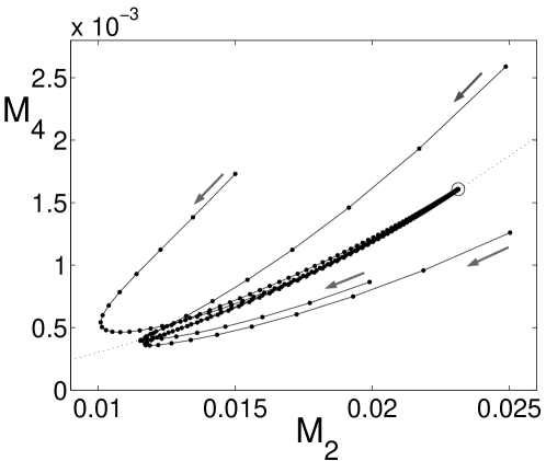
Figure 3: Trajectories of 300 oscillators ($K=0.7$) in the phase space of ${\cal M}_{2}$ and ${\cal M}_{4}$, started from four different sets of values, but with the same natural frequency distribution. Each dot is separated by 0.1 in time (arrows indicate the direction of increasing time). Initially, $g(\omega)$ and $f(\theta)$ have no correlations. In all cases, both moments decrease first (during $t<1$), and then gradually increase toward a steady state [(${\cal M}_{2}^{ss},{\cal M}_{4}^{ss}$) = (2.3131$\times 10^{-2}$, 1.6076$\times 10^{-3}$) marked by a circle]. The latter slow evolution occurs along a “slow manifold”, which nearly coincides with the curve for Gaussian distributions (dotted line, ${\cal M}_{4}-3{\cal M}_{2}^{2}=0$).

References

- [1] Ariaratnam, J. T. & S. H, Strogatz, S. H. [2001] “Phase Diagram for the Winfree Model of Coupled Nonlinear Oscillators”, Phys. Rev. Lett., 86, 4278-4281.
- [2] Buck, J. [1988] “Synchronous rhythmic flashing of fireflies II”, Quart. Rev. Biol., 63, 265-289.
- [3] Chapman, S. & Cowling, T. G. [1970] “The Mathematical Theory of Non-uniform Gases”, Cambridge University Press, Cambridge.
- [4] Ertl, G. [1991] “Oscillatory Kinetics and Spatio-Temporal Self-Organization in Reactions at Solid Surfaces”, Science, 254, 1750-1755.
- [5] Ermentrout, G. B. & Kopell, N. [1984] “Frequency plateaus in a chain of weakly coupled oscillators. I.”, SIAM J. Math. Anal., 15, 215-237.
- [6] Gear, C. W., Kevrekidis, I. G. & Theodoropoulos, C. [2002] ““Coarse” Integration/Bifurcation Analysis via Microscopic Simulators: Micro-Galerkin methods”, Comp. Chem. Engng., 26, 941-963.
- [7] Gear, C. W. & Kevrekidis, I. G. [2003a] “Projective Methods for Stiff Differential Equations: Problems with gaps in their eigenvalue spectrum”, SIAM J. Sci. Comp., 24, 1091-1106.
- [8] Gear, C. W. & Kevrekidis, I. G. [2003b] “Telescopic Projective Integrators for Stiff Differential Equations”, J. of Comp. Phys., 187, 95-109.
- [9] Gear, C. W., Li, J. & Kevrekidis, I. G. [2003c] “The gap-tooth method in particle simulations”, Phys. Lett. A, 316, 190-195.
- [10] Gear, C. W. & Kevrekidis, I. G. [2004a] “Computing in the Past with Forward Integration”, Phys. Lett. A, 321, 335-343.
- [11] Gear, C. W. & Kevrekidis, I. G. [2004b] “Constraint-defined Manifolds: a Legacy-Code Approach to Low-Dimensional Computations”, J. Sci. Comp., in press.
- [12] Gear, C. W., Kaper, T. J., Kevrekidis, I. G. & Zagaris, A. [2004c] “Projecting on a Slow Manifold: Singularly Perturbed Systems and Legacy Codes”, submitted to SIADS; e-print, physics/0405074 at arXiv.org.
- [13] Gray, C. M., König, P., Engel, A. K. & Singer, W. [1989] “Oscillatory responses in cat visual cortex exhibit inter-columnar synchronization which reflects global stimulus properties”, Nature, 338, 334-337.
- [14] Hummer, G. & Kevrekidis, I. G. [2003] “Coarse molecular dynamics of a peptide fragment: free energy, kinetics and long time dynamics computations”, J. Chem. Phys., 118, 10762-10773.
- [15] Kevrekidis, I. G., Gear, C. W., Hyman, J. M., Kevrekidis, P. G., Runborg, O. & Theodoropoulos, C. [2003] “Equation-free coarse-grained multiscale computation: enabling microscopic simulators to perform system-level tasks”, Comm. Math. Sciences, 1(4), 715-762; also physics/0209043 at arXiv.org.
- [16] Kevrekidis, I. G., Gear, C. W. & Hummer, G. [2004] “Equation-free: the computer-assisted analysis of complex, multiscale systems”, AIChE J., 50 (7), 1346-1354.
- [17] Kelley, C. T. [1995] “Iterative Methods for Linear and Nonlinear Equations” (Frontiers in Applied Mathematics, Vol. 16), SIAM, Philadelphia.
- [18] Kiss, I. Z., Zhai, Y. & Hudson, J. L. [2002] “Emerging Coherence in a Population of Chemical Oscillators”, Science, 296, 1676-1678.
- [19] Kotz, S. & Nadarajah, S. [2000] “Extreme Value Distributions”, Imperial College Press, London.
- [20] Kuramoto, Y. [1975] “International Symposium on Mathematical Problems in Theoretical Physics”, Edited by H. Arakai, Lecture Notes in Physics, Vol. 39, (Springer, New York), p. 420.
- [21] Kuramoto, Y. [1984] “Chemical Oscillations, Waves, and Turbulence”, Springer-Verlag.
- [22] Makeev, A. G., Maroudas, D., Panagiotopoulos, A. Z. & Kevrekidis, I. G. [2002] “Coarse bifurcation analysis of kinetic Monte Carlo simulations: A lattice gas model with lateral interactions”, J. Chem. Phys., 117, 8229-8240.
- [23] Manrubia, S. C., Mikhailov, A. S. & Zanette, D. H. [2004] “Emergence of Dynamical Order”, World Scientific, Singapore.
- [24] Moon, S. J., Ghanem, R. & Kevrekidis, I. G. [2005] “A coarse-grained approach to finite-dimensional coupled oscillator dynamics”, in preparation.
- [25] Néda, Z., Ravasz, E., Brechet, Y., Vicsek, T. & Barabási, A. L., “Self-organizing processes: The sound of many hands clapping”, Nature, 403, 849-850.
- [26] Oliva, R. A. & Strogatz, S. H. [2001] “Dynamics of a large array of globally coupled lasers with distributed frequencies”, Int. J. Bifurcation Chaos, 11, 2359-2374.
- [27] Ryckaert, J. P., Ciccotti, G. & Berendsen, H. [1977] “Numerical Integration of the Cartesian equations of motion of a system with constraints: Molecular Dynamics of N-alkanes”, J. Comp. Phys., 23, 327-341.
- [28] Samaey, G., Kevrekidis, I. G. & Roose, D. [2004] ”Patch dynamics with buffers for homogenization problems”, submitted to J. Comp. Phys.
- [29] Siettos, C., Graham, M. D. & Kevrekidis, I. G. [2003] “Coarse Brownian dynamics for nematic liquid crystals: Bifurcation, projective integration and control via stochastic simulation”, J. Chem. Phys., 118, 10149-10157.
- [30] Shroff, G. M. & Keller, H. B. [1993] “Stabilization of unstable procedures: The recursive projection method”, SIAM J. Numer. Anal., 30, 1099-1120.
- [31] Strogatz, S. [2000] “From Kuramoto to Crawford: exploring the onset of synchronization in populations of coupled oscillators”, Physica D, 143, 1-20.
- [32] Theodoropoulos, C., Qian, Y. H. & Kevrekidis, I. G. [2000] ““Coarse” stability and bifurcation analysis using time-steppers: A reaction-diffusion example”, Proc. Natl. Acad. Sci. USA, 97, 9840-9843.
- [33] Torrie, G. M. & Valleau, J. P. [1974] “Monte Carlo free energy estimates using non-Boltzmann sampling: application to the sub-critical Lennard Jones fluid”, Chem. Phys. Lett., 28, 578-581.
- [34] Walker, T. J. [1969] “Acoustic synchrony: two mechanisms in the snowy tree cricket”, Science, 166, 891-894.
- [35] Winfree, A. T. [1967] “Biological rhythms and the behavior of populations of coupled oscillators”, J. Theor. Biol., 16, 15-42.
- [36] Wiesenfeld, K., Colet, P. & Strogatz, S. H. [1996] “Synchronization Transitions in a Disordered Josephson Series Array”, Phys. Rev. Lett., 76, 404-407.
- [37] A numerical bifurcation software available from http://indy.cs.concordia.ca/auto/
- [38] A package using backward differentiation formula methods to solve a system of DAEs or ODEs; available from http://www.engineering.ucsb.edu/cse/software.html