Birhythmicity, Synchronization, and Turbulence in an Oscillatory System with Nonlocal Inertial Coupling

Abstract

We consider a model where a population of diffusively coupled limit-cycle oscillators, described by the complex Ginzburg-Landau equation, interacts nonlocally via an inertial field. For sufficiently high intensity of nonlocal inertial coupling, the system exhibits birhythmicity with two oscillation modes at largely different frequencies. Stability of uniform oscillations in the birhythmic region is analyzed by means of the phase dynamics approximation. Numerical simulations show that, depending on its parameters, the system has irregular intermittent regimes with local bursts of synchronization or desynchronization.

and

1 Introduction

Beginning with the pioneering contributions by Kuramoto [1] and Winfree [2], studies of synchronization and spatiotemporal chaos (turbulence) in populations of coupled active oscillators have developed into a classical field of research. In chemical systems, each oscillator represents a reaction element and coupling between such elements is usually due to diffusion of reactants in the system. This coupling extends only within a short diffusion length and is therefore local. The complex Ginzburg-Landau equation is the canonical model for oscillatory systems with local coupling near a supercritical Hopf bifurcation. In surface chemical reactions [3], reaction elements are however additionally interacting through the gas phase where instantaneous complete mixing occurs. As a result, global coupling between chemical oscillators arises [4]. Moreover, global delayed feedbacks through the gas phase could be artificially introduced to control turbulence in surface reactions [17, 18, 19, 26, 27, 28]. A special class of systems are arrays of active oscillators that do not directly interact one with another, but are all coupled to a single diffusing field (in biochemistry, an example of such a system would be provided by arrays of allosteric enzymes interacting through a chemical messenger [5]). Adiabatically eliminating this field, models with nonlocal coupling between the oscillators, described by a finite-range integral, were derived [6, 9]. Investigations of nonlocally coupled oscillator arrays have revealed that such form of coupling does not always synchronize neighbouring oscillators and discontinuous distributions with scaleless fractal structure can develop [8, 9]. Spatiotemporal chaos can develop in such systems even in the Benjamin-Feir stable regime [12] and spiral waves with phase-randomized cores can exist here [15, 14].

Furthermore, arrays with both local and nonlocal coupling between oscillators are possible. This situation is characteristic, for example, for surface chemical reactions. In such systems, diffusion provides local coupling between neighbouring surface oscillators, whereas much faster heat conduction is responsible for nonlocal coupling between them.

Recently, Tanaka and Kuramoto [16] have shown how, in the vicinity of a supercritical Hopf bifurcation, the description of arrays of nonlocally coupled oscillators can be reduced to the complex Ginzburg-Landau equation with nonlocal coupling. Because of the critical slowing down near the bifurcation point, the coupling is effectively instantaneous in the reduced description.

In realistic systems, which are not too close to the Hopf bifurcation, one can however also encounter the opposite situation, with a very slow inertial field giving rise to nonlocal coupling. The aim of our study is to analyze what new effects, primarily due to slow nonlocal coupling, are possible in this class of systems. For our investigations, we have chosen an abstract model of the complex Ginzburg-Landau equation interacting with an additional slow field, so that the coupling is nonlocal both with respect to space and time. We expect that the behaviour found in this general model would be typical for a broad class of realistic systems.

The principal effect of coupling inertiality is that birhythmicity, leading to chaotic intermittency, can develop in such systems. In contrast to the birhythmicity in reaction-diffusion systems near a pitchfork-Hopf bifurcation (see [20, 21]), the two oscillatory states are characterized here by very different frequencies and oscillation amplitudes. For the rapid oscillatory state, the additional field responsible for the inertial long-range coupling is almost absent and only diffusive local coupling between the oscillators is important. In slow oscillations, the elements are however entrained by the long-range inertial field.

Depending on the parameters, two new kinds of intermittency are found here. When rapid oscillations are modulationally unstable and give rise to turbulence, spatial regions occupied by slow entrained oscillations spontaneously develop and die out in the medium. They can be interpreted as bursts of synchronization on a turbulent background. On the other hand, relatively small, irregularly evolving islands filled with rapid turbulence can persist on the background of slow almost uniform oscillations. They can be therefore described as bursts of desynchronization on the background of regular slow oscillations. Our analysis of such phenomena is based on the phase dynamics approximation, derived for the birhythmic system. It is complemented by 1D and 2D numerical simulations.

2 The Model

The investigated model describes a system of diffusively coupled active oscillators coupled to an additional inertial diffusive field. Introducing the local complex oscillation amplitude $\eta(x,t)$ and denoting as $z(x,t)$ the additional complex-valued diffusive field, we have therefore a system of two equations

$$\dot{\eta} = \quad(1+\mathrm{i}\omega)\eta-(1+\mathrm{i}\alpha)|\eta|^{2}\eta+(1+\mathrm{i}\beta)\nabla^{2}\eta+K(z-\eta)$$ (1a)

$$\tau\dot{z} = \quad\eta-z+l^{2}\nabla^{2}z$$ (1b)

The additional last term in the complex Ginzburg-Landau equation (1a) takes into account coupling of the oscillatory subsystem with the field $z$ whose evolution obeys equation (1b); $K$ is the respective coupling constant. The equations are brought into a dimensionless form by choosing the characteristic diffusion length in the oscillatory subsystem as the length unit and taking the characteristic relaxation time scale of the oscillators as the time unit. The parameters $\tau$ and $l$ determine characteristic time and length scales of the additional field $z$. We assume that this field is inertial ($\tau\gg 1$) and slowly varying in space ($l\gg 1$).

The linear equation (1b) can easily be solved as

$$z(x,t)=\int_{-\infty}^{\infty}\int_{0}^{t}G(x-x^{\prime},t-t^{\prime})\eta(x^{\prime},t^{\prime})dx^{\prime}dt^{\prime}.$$ (2)

where the kernel is given by

$$G(x,t)=\frac{1}{2\tau\sqrt{\pi Dt}}\exp\left(-\frac{x^{2}}{4Dt}-\frac{t}{\tau}\right).$$ (3)

Substituting this into equation (1a), we obtain an equivalent integro-differential form of the considered model,

$$\dot{\eta} = (1+\mathrm{i}\omega)\eta-(1+\mathrm{i}\alpha)|\eta|^{2}\eta+(1+\mathrm{i}\beta)\nabla^{2}\eta$$ (4)

$$+K\int_{-\infty}^{\infty}\int_{0}^{t}G(x-x^{\prime},t-t^{\prime})\left[\eta(x^{\prime},t^{\prime})-\eta(x,t)\right]dx^{\prime}dt^{\prime}$$

We see that, besides of diffusion, the model also includes an additional coupling, nonlocal both with respect to space and time.

Note that very close to a supercritical Hopf bifurcation all processes become fast as compared to the relaxation time scale of individual oscillators, because this time is inversely proportional to the distance from the bifurcation point (critical slowing down). However, it is known that the complex Ginzburg-Landau equation yields qualitatively correct description even relatively far from the bifurcation. Equations (1) and (4) can be viewed as providing a simple model of an oscillating system coupled to an inertial diffusive field.

3 Birhythmicity

The system described by equations (1) is birhythmic, i.e. it can have two different oscillatory uniform states. Assuming that $\eta(t)=\rho e^{-\mathrm{i}\gamma t}$ and $z(t)=re^{-\mathrm{i}\gamma t}$ and substituting this into equations (1a) and (1b), we obtain a cubic equation for the oscillation frequency $\gamma$,

$$\tau^{2}\gamma^{3}+\tau^{2}(\omega-\alpha+\alpha K)\gamma^{2}+(1+\tau K)\gamma+\omega-\alpha=0.$$ (5)

When the frequency $\gamma$ is known, the oscillation amplitude $\rho$ of the field $\eta$ is given by

$$\rho^{2}=1-\frac{K\tau^{2}\gamma^{2}}{1+\tau^{2}\gamma^{2}}.$$ (6)

The respective oscillation amplitude of the field $z$ is

$$r=\frac{\rho}{\sqrt{1+\tau^{2}\gamma^{2}}}.$$ (7)

Depending on its parameters, equation (5) can have either one or three real roots. The three roots correspond to three possible modes of uniform oscillations with frequencies $\gamma_{1,2,3}$, such that $\gamma_{1}<\gamma_{2}<\gamma_{3}$. It can be checked that oscillations with the middle frequency $\gamma_{2}$ are always unstable. In contrast to this, uniform oscillations with frequencies $\gamma_{1}$ and $\gamma_{3}$ are possible (but may still be unstable with respect to nonuniform perturbations, see the discussion below).

Figure 1 shows the region in the parameter planes ($\alpha-\omega,K$) and ($\tau,K$) where birhythmicity exists. The birhythmicity is possible only for sufficiently strong coupling $K$. Moreover, it develops only if the characteristic time $\tau$ of the field $z$ is sufficiently large (Fig. 1).

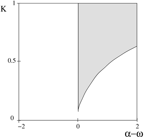
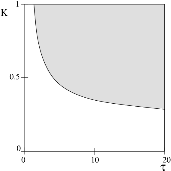
Figure 1: Birhythimicity regions (gray) for the model (1) in the parameter planes $(\alpha-\omega,K)$ and $(\tau,K).$ The fixed parameters are $\tau=10$ in the first diagram and $\omega=2,\alpha=2.5$ in the second diagram. The boundaries of the displayed regions do not depend on the parameter $\beta$ of the model.

Numerical solutions of equation (5) are displayed in Fig. 2. If the parameter $\alpha$ is kept constant and the coupling strength $K$ is varied (Fig. 2), birhythmicity is found inside the interval $0.4<K<1$. When $K\geq 1,$ the system has a stable stationary state coexisting with oscillations. The dependence of the effective oscillation frequency $\gamma$ on the difference $\alpha-\omega$ for $K=0.5$ is shown in Fig.2. Two stable limit cycles coexist within the interval $-0.1<\alpha-\omega<0.8$.

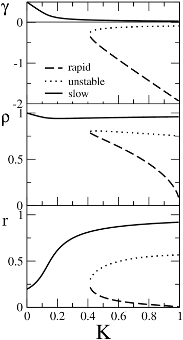
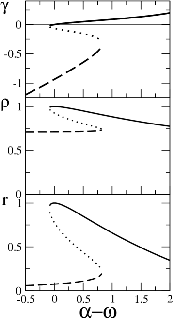
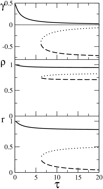
Figure 2: Bifurcation diagrams. Frequencies $\gamma$ of uniform oscillations, together with the respective amplitudes $\rho=|\eta|$ and $r=|z|$ as functions of $K$, $\alpha-\omega$ and $\tau$ for slow (bold line), rapid (dashed) and absolutely unstable (dotted) uniform oscillation modes. The parameters are (a) $\omega=2,\alpha=2.5,\tau=10$ (b) $\omega=2,K=0.5,\tau=10,$ (c) $\omega=2,\alpha=2.5,K=0.5.$

The difference between the two limit cycles becomes clear if we compare the amplitudes of oscillations of the fields $\eta$ and $z$ which are presented below in the same figures. As we have already observed, at $K=0$ only one oscillating mode is present, as we are in this limit reduced to the standard CGLE. Thus, we can expect that the branch starting at $K=0$ (which is the upper one in the bifurcation diagrams of Fig. 2) would have the strongest similarities to the CGLE, even though for finite $K$ it would be affected by the coupling to the second field. This branch is characterized by a large amplitude of the field $\eta$, which never gets significantly smaller than 1. The corresponding frequency is quite small, starting from $\gamma=0.5$ at $K=0$ and slowly decreasing as $K$ increases. Below, we refer to this attractor as corresponding to the slow limit cycle.

In contrast to this, oscillations in the lower branch have a smaller amplitude $\rho$, which decreases for higher coupling strengths $K$ and eventually vanishes at $K=1$. Note that $\gamma$ is negative for this mode and therefore such oscillations are counter-rotating with respect to the upper branch. The frequency varies significantly for this mode. Inside the birhythmicity interval, the frequency of such rapid limit cycle is always much larger (in its magnitude) than the frequency of the slow mode. A characteristic feature of the rapid limit cycle is that the amplitude $r$ of the field $z$ is very small here. This is because the oscillations of the field $\eta$ are so rapid here that the inertial field $z$ cannot respond to them. Hence, the coupling term $Kz$ in the system (1) is almost negligible for the rapid limit cycle so that the nonlocal coupling is ineffective and oscillators interact only via the local diffusional coupling in this mode.

4 The Phase Dynamics Approximation

Above, uniform oscillations in the model have been discussed. Now, we want to consider the properties of almost uniform oscillations, characterized by small phase gradients. Because the system is invariant with respect to the uniform shift of all phases, the evolution of phase distributions with small phase gradients should be slow, in contrast to fast local relaxation of the amplitude perturbations. Therefore, a reduced description, known as the phase dynamics approximation, can be constructed in such cases [1]. When birhythmicity is present, the coefficients of the phase dynamics equation are different for the two oscillation modes.

The derivation of the phase dynamics equation for this system is lengthy and has been performed by using a computer program for algebraic calculations (Mathematica). Below in this section we show the scheme of derivation and discuss the results. The complete derivation is presented in Appendix A.

We define the phases ($\phi$ and $\varphi$) and amplitudes ($\rho$ and $r$) of complex fields $\eta$ and $z$ as $\eta=\rho e^{\mathrm{i}\phi}$, $z=re^{\mathrm{i}\varphi}$. It is convenient to use instead of $\phi$ and $\varphi$ the variables $\psi=\phi-\varphi$ and $\Theta=\phi+\varphi$. Note that the phase sum $\Theta$ is the slow variable in this system. The phases of the two fields are rigidly correlated in the uniform state and their difference $\psi$ undergoes rapid relaxation, similar to oscillation amplitudes $\rho$ and $z$.

In terms of the new variables, the model (1) takes the form

$$\dot{\rho} = \rho-\rho^{3}+Kr\cos\psi-K\rho+\rho\left(-\displaystyle\frac{\nabla\Theta^{2}}{4}+\displaystyle\frac{1}{2}\beta\nabla^{2}\Theta\right)$$ (8a)

$$\dot{r} = \displaystyle\frac{\rho}{\tau}\cos{\psi}-\displaystyle\frac{r}{\tau}-\displaystyle\frac{l^{2}}{4\tau}r\nabla\Theta^{2}$$ (8b)

$$\dot{\psi} = -\omega+\alpha\rho^{2}-\left(\displaystyle\frac{kr}{\rho}+\displaystyle\frac{\rho}{\tau r}\right)\sin\psi+\displaystyle\frac{\beta}{4}\nabla\Theta^{2}+\displaystyle\frac{1}{2}\left(1-\displaystyle\frac{l^{2}}{\tau}\right)\nabla^{2}\Theta$$ (8c)

$$\dot{\Theta} = -\omega+\alpha\rho^{2}-\left(\displaystyle\frac{kr}{\rho}-\displaystyle\frac{\rho}{\tau r}\right)\sin\psi+\displaystyle\frac{\beta}{4}\nabla\Theta^{2}+\displaystyle\frac{1}{2}\left(1+\displaystyle\frac{l^{2}}{\tau}\right)\nabla^{2}\Theta$$ (8d)

Suppose now that the birhythmic system is close to one of its two oscillatory states, characterized by some amplitudes $\rho_{0}$ and $r_{0}$, and the relative phase $\psi_{0}$, whereas the phase sum $\Theta$ remains arbitrary. If the phase sum $\Theta$ is slowly varying in space, the variables $\rho$, $r$ and $\psi$ would only slightly deviate from their equilibrium values. Therefore, we can introduce small perturbations of such variables, $\rho=\rho_{0}+\delta\rho$, $r=r_{0}+\delta r$, $\psi=\psi_{0}+\delta\psi$, and linearize the equations for with respect to such perturbations. The linearized evolution equation for the phase $\Theta$ is

$$\dot{\Theta} = -\omega+\alpha\rho_{0}^{2}-\left(\frac{Kr_{0}}{\rho_{0}}-\frac{\rho_{0}}{\tau r_{0}}\right)\sin\psi_{0}$$ (9)

$$+ \delta\rho\left[2\alpha\rho_{0}+\left(\frac{Kr_{0}}{\rho_{0}^{2}}+\frac{1}{\tau r_{0}}\right)\sin\psi_{0}\right]$$

$$+ \delta r\left(-\frac{K}{\rho_{0}}-\frac{\rho_{0}}{\tau r_{0}^{2}}\right)\sin\psi_{0}+\delta\psi\left(-\frac{Kr_{0}}{\rho_{0}}+\frac{\rho_{0}}{\tau r_{0}}\right)\cos\psi_{0}$$

$$+ \frac{\beta}{4}\nabla\Theta^{2}+\frac{1}{2}\left(1+\frac{l^{2}}{\tau}\right)\nabla^{2}\Theta$$

The linearized equations for the variables $\delta\rho,\delta r,\delta\psi$ can be solved in the adiabatic approximation, because these fast variables are adjusting to slow variation of $\Theta$. Substituting the result into (9), a closed evolution equation for the phase variable $\Theta$ is derived. This equation has the form:

$$\dot{\Theta}=C_{0}+C_{1}(\nabla\Theta)^{2}+C_{2}\nabla^{2}\Theta$$ (10)

The analytical expressions for the coefficients $C_{0},$ $C_{1}$ are given in Appendix A. Note that inside the birhythmic region there are two uniform oscillation modes with different $\rho_{0}$, $r_{0}$, and $\psi_{0}$, and thus with different values of these coefficients.

The most important coefficient is $C_{2}$ because its sign controls stability of uniform oscillations with respect to phase modulation (the Benjamin-Feir instability). If $C_{2}>0$, uniform oscillations are stable, if $C_{2}<0$ they are unstable. We have computed this coefficient as functions of several model parameters, by using the obtained analytical expressions. The computed dependences are shown in Fig. 3. Two different branches correspond to the two different limit cycles. The upper curves in Fig. 3(a,b,d) are for the slow mode, whereas the lower curves are for the rapid oscillations. In Fig. 3(c), the upper curves correspond to the slow mode for larger values of the parameter $l$.

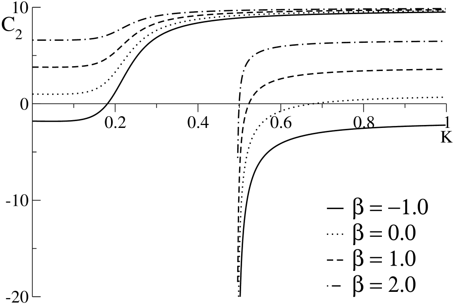
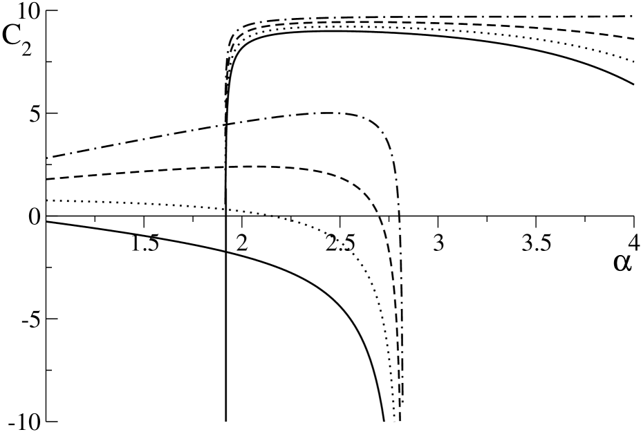
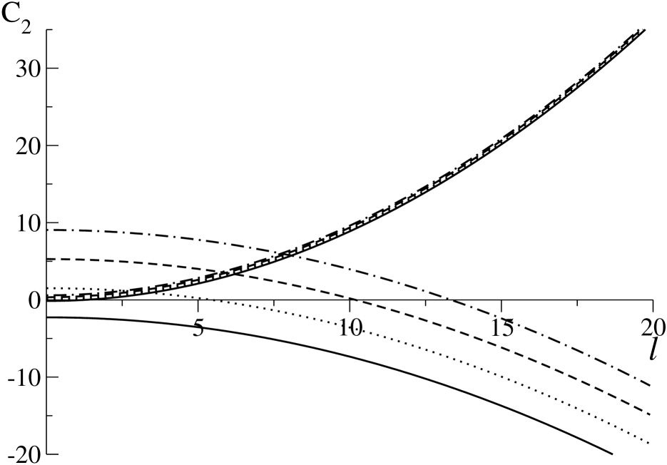
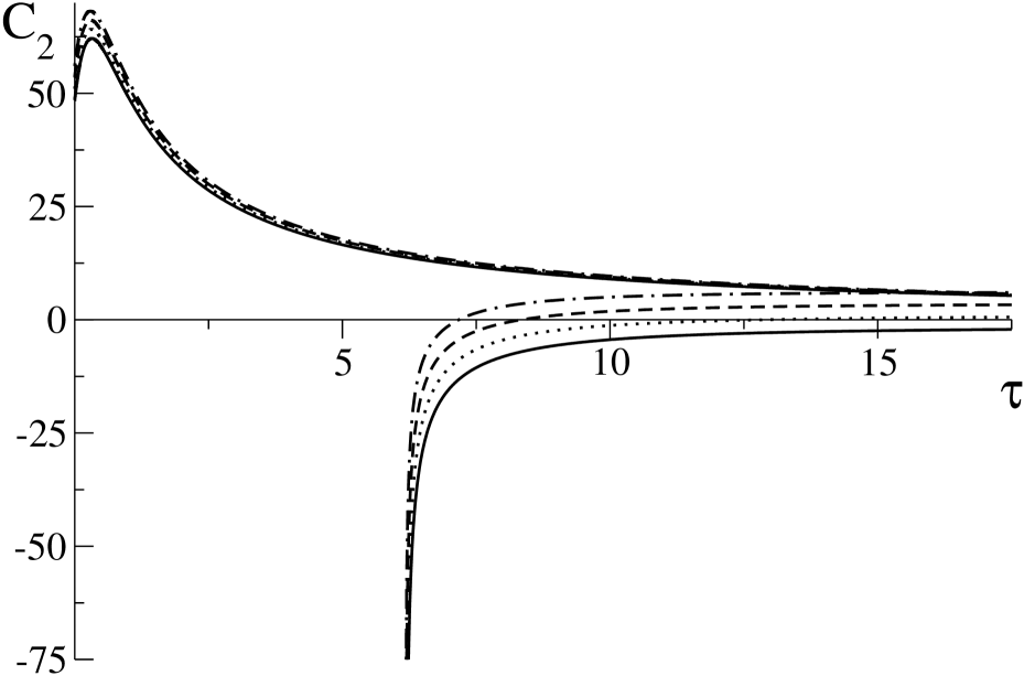
Figure 3: The coefficient $C_{2}$ of the phase dynamics equations as functions of $K,\alpha,l$ and $\tau$ for several different values of the parameter $\beta$. The upper branches in (a,b,d) and for the larger values of $l$ in (c) correspond to slow oscillations, the lower branches are for the rapid oscillations. The oscillations are unstable if $C_{2}<0$. The parameters are (a) $\alpha=2.5,$ $l=10$, $\tau=10,$ (b) $K=0.5,l=10,\tau=10,$ (c) $\alpha=2.5,$ $K=0.5,$ $\tau=10,$ (d) $\alpha=2.5,$ $K=0.5,$ $l=10;$ for all curves $\omega=2.$

Examining these plots, several observations can be made: Slow mode oscillations are always stable inside the birhythmic region, even when the system without coupling is Benjamin-Feir unstable (i.e., $1+\alpha\beta<0$ and therefore $C_{2}<0$ at $K=0$). In contrast to this, rapid oscillations are always unstable when the condition $1+\alpha\beta<0$ is satisfied. Moreover, they are unstable near the boundary of the birhythmic region, at which they first appear, even when this condition is violated. Increasing the diffusion length $l$ of the field $z$ favors instability of rapid uniform oscillations.

5 Numerical Simulations

To investigate nonlinear spatiotemporal dynamics in the considered model, simulations of equations (1a) and (1b) have been performed. For numerical integration of these equations, the fourth-order Runge-Kutta algorithm has been used. The mesh size for space discretization and the time step have been chosen to optimize the computational time for each parameter choice. Since the diffusion length and the diffusion constant of the oscillatory field have both been chosen to be equal to unity, $\Delta x$ varied between 0.3 and 0.5, while $\Delta t$ could vary between $(\Delta x)^{2}/5$ and $(\Delta x)^{2}/2$. Both one- and two-dimensional systems were investigated. No-flux boundary conditions were employed. Initial conditions varied depending on a particular simulation.

To display the results of one-dimensional simulations, space-time diagrams have been constructed. In such diagrams, time always runs along the horizontal axis and the vertical axis is corresponding to the spatial coordinate. In two dimensions, snapshots at some time moments and space-time diagrams showing evolution of the pattern along some linear cross-section are presented. The patterns are shown by using a gray scale where the white color encodes the smallest and the black color the largest values of the displayed variable.

First, the behavior of fronts separating spatial regions with two different oscillatory states in the birhythmic system has been studied (Fig. 4). The front travels towards the slow oscillating region, in such a way that the system ends up with uniform oscillations of the rapid mode. Its propagation is characterized by periodic appearance of amplitude defects which occur when the phase difference between the two oscillating regions equals $2\pi$ (see Fig 4(b)). The front moves at a constant velocity which depends on the parameters of the system. Fig. 5 shows the dependence of the front velocity on the parameter $\alpha$ for several values of the coupling strength $K$. In Fig. 5, the dependence of the front propagation velocity on the frequency difference $\Delta\gamma=\gamma_{3}-\gamma_{1}$ of two uniform oscillatory modes is presented. The front always moves faster when this difference is increased.

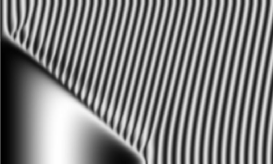
(a) Re$(\eta)$

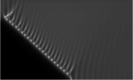
(b) $|\eta|$

Figure 4: Spatiotemporal diagrams showing front propagation in the birhythmic system with $\omega=2,\alpha=2.5,\beta=1,K=0.5,l=10,$ and $\tau=10.$ The total system length is $L=120$ and the total displayed time interval is $T=300$. Bright regions correspond to small values of displayed variables. Time runs from left to right along the horizontal axis, the spatial coordinate is varied in vertical direction.

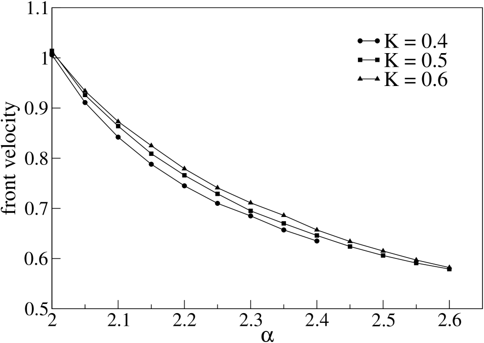
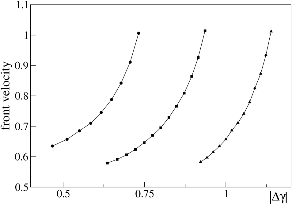
Figure 5: Front velocity as functions of the parameter $\alpha$ and difference $\Delta\gamma$ of oscillation frequencies in the two modes in the birhythmic regime. The fixed parameters are $\omega=2,\beta=1,l=10,$ and $\tau=10.$

As follows from the stability analysis of uniform oscillatory states (see, e.g., Fig. 3), rapid oscillations should be unstable with respect to phase modulation near the birhythmicity boundary and complex spatiotemporal regimes can be expected there. We have performed a series of numerical simulations, exploring pattern formation in the system within the intervals $2.55<\alpha<2.8$ and $-1<\beta<2.5$, while keeping fixed the other parameters ($\omega=2,K=0.5,l=10,$ and $\tau=10$). Each simulation started from independently chosen, completely random initial conditions.

Figure 6 is a schematic summary of these numerical investigations. The solid line is the stability boundary of rapid oscillations ($C_{2}=0$); rapid oscillations are unstable below this boundary. Slow oscillations are always stable in the considered region. Simulations have been performed for a set of parameter values indicated by symbols in this diagram.

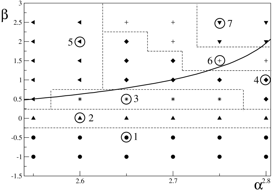
Figure 6: Schematic phase diagram. Numerical simulations of the one-dimensional model were performed at the values of $\alpha$ and $\beta$ indicated by symbols in this diagram. Depending on the observed properties of patterns, the diagram is divided into regions 1 to 6. The circles indicate the values of these parameters used to produce a typical patterns for the corresponding region, displayed in Fig. 7. The solid line shows the stability boundary of rapid uniform oscillations, given by the condition $C_{2}=0$. Other parameters are $\omega=2,K=0.5,l=10,$ and $\tau=10$.

Comparing properties of observed patterns, we can qualitatively divide them into several groups occupying different regions in the parameter plane. Each group is marked by its own symbol and the respective regions in Fig. 6 are numbered. Examples of typical spatiotemporal patterns, observed in one-dimensional simulations within each region, are displayed in Fig. 7. These simulations were all performed for a system of the total length $L=200$ and for a total time varying between 500 to 3000 time units. To clearly present the observed patterns, only parts of their entire evolution are however displayed.

	Re$(\eta)$	$|\eta|$	$|z|$
1
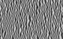
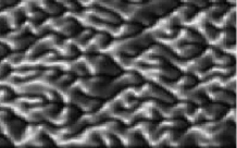
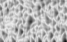
2
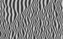
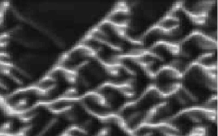
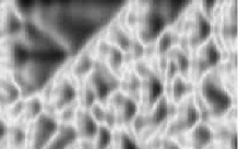
3
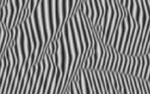
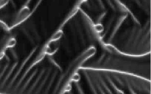
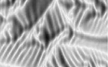
4
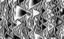
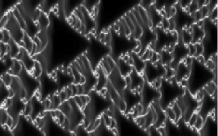
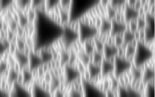
5
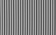
6
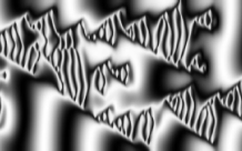
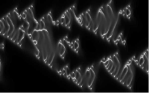
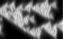
7

Figure 7: Spatiotemporal diagrams displaying evolution of Re($\eta$), $\rho=|\eta|$ and $r=|z|$ in typical patterns observed in the regions 1-6 for the one-dimensional system. The respective parameter values are given in Fig. 6. The displayed space and time intervals are (1) $L=100,$ $T=166,$ (2) $L=100,$ $T=166,$ (3) $L=100,$ $T=250,$ (4) $L=200,$ $T=500,$ (5) $L=100,$ $T=250,$ (6) $L=200,$ $T=500,$ and (7) $L=200,$ $T=250.$ The contrast level is adjusted individually in each plot to ensure best visualization of the pattern.

In region 1, the slow limit cycle is Benjamin-Feir stable, while the rapid limit cycle is unstable. The system is found here in the regime of fully developed amplitude turbulence characterized by creation of multiple amplitude defects. Increasing parameter $\beta$, we enter a region 2 closer to the stability boundary where turbulence becomes intermittent. We observed the emergence of larger groups of synchronized oscillators which become able to reach the rapid limit cycle and perform harmonical oscillations for several periods. Inside the small parameter region 3 near the stability boundary, the frequency and the amplitude of oscillations correspond almost everywhere to those of the rapid limit cycle. However, the system does not undergo complete synchronization. Lines of amplitude defects travelling through the system act as wave sources here.

In regions 5 and 7, both lying above the stability boundary of rapid oscillations, uniform oscillations are observed starting from random initial conditions. The oscillations are rapid inside region 5 and slow inside region 7. These two domains are separated by regions 4 and 6 in the parameter plane, where competition between two oscillation mode takes place leading to complex spatiotemporal regimes.

The patterns inside region 4 are characterized by a background of rapid chaotic oscillations, with small amplitude and numerous amplitude defects. On this highly desynchronized background, bursts of synchronization emerge. Such bursts consist of large groups of elements which suddenly start to oscillate together with a large amplitude and a small frequency corresponding to the stable slow limit cycle. However, these groups do not keep synchronized over a long time: after less than one oscillation period the turbulence overwhelms again. As already noticed in our discussion of birhythmicity, the amplitude of the coupling field $z$ is very small in the rapid limit cycle, while in the slow limit cycle it gets a larger value comparable to the amplitude of $\eta$. Analyzing patterns in region 4, it can be seen that during the synchronization bursts, the amplitude $|z|$ is indeed much larger than in the turbulent background. Note that such patterns with synchronization bursts have also been observed for some parameter values below the stability boundary of rapid uniform oscillations.

Region 6 lies near region 7, where slow uniform oscillations are winning the competition. Here, the patterns can be described as exhibiting bursts of desynchronization on the background of slow uniform oscillations. Inside such bursts, the coupling field $z$ is strongly decreased in amplitude and only short-range diffusive coupling between oscillators is effective.

To further illustrate this regime, phase portraits of the patterns in region 6 were constructed at different time moments. Fig. 8 shows several subsequent snapshots from the recorded video. Each point in a phase portrait represents a state of one of the oscillators. The spatial information (i.e., spatial distances between the displayed oscillators) is lost in this representation, but the motions performed by the oscillator population are seen more clearly. The two circles indicate the two coexisting limit cycles. The cycle with a smaller oscillation amplitude is rapid, whereas the cycle with a larger amplitude is slow.

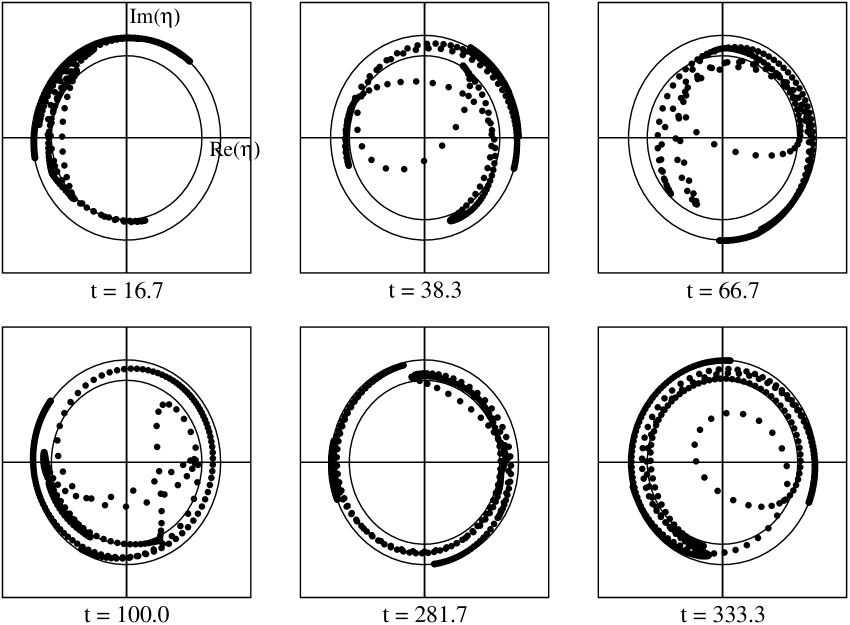
Figure 8: Selected snapshots of the phase portraits for the pattern 6 in Fig. 7. The circles show two different limits cycles in the birhythmic system.

We can see from these snapshots that the system is usually divided into two groups of oscillators, occupying the two coexisting attractors (limit cycles). Some oscillators are found in the vicinity of the origin $\eta=0$. They correspond to amplitude defects generated at the border between spatial regions with different oscillation frequencies (bright dots in the spatiotemporal plot of $|\eta|$ for pattern 6 in Fig. 7). Such defects are not present at all times, and the respective points are not, for example, seen in the phase portraits at $t=16.7$ and $t=281.7$. The oscillators sitting on the rapid limit cycle with the smaller amplitude belong to the desynchronization bursts.

For selected parameter values, two-dimensional simulations of the system have additionally been performed. Figure 9 displays the behavior of a two-dimensional system at the same parameters as for the pattern 3 in Fig. 7. The space-time diagrams in the right panels show the pattern development along a horizontal cross section. Starting from random initial conditions, a population of rotating spiral waves develops. After a transient, a stable configuration of rotating spirals is reached in two dimensions.

Figure 10 shows two-dimensional patterns corresponding to synchronization bursts (pattern 4 in Fig. 7). Inside such a burst, occupying for example the left central region in the left panels, the coupling field $z$ is increased in magnitude. The space-time diagrams (right panels) reveal that the synchronized regions with slow oscillations have only relatively short lifetimes and are replaced by irregular rapid oscillations. However, they appear again and again in the course of time.

Re$(\eta)$
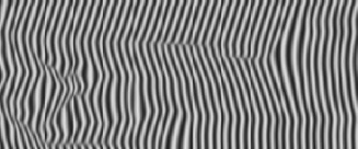
$|\eta|$
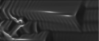
$|z|$

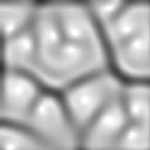
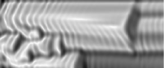
Figure 9: Multiple spiral waves in a two-dimensional system of size $120\times 120;$ the same parameter values as for the pattern 3 in Fig. 7. The right panels are space-time plots showing evolution of the pattern along one horizontal cross section; the displayed time interval is $T=480$

Re$(\eta)$
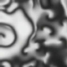
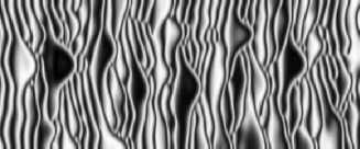
$|\eta|$
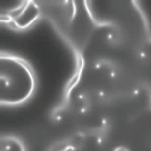
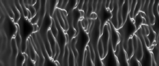
$|z|$

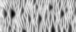
Figure 10: Bursts of synchronization in a two-dimensional system of size $120\times 120;$ the same parameter values as for the pattern 4 in Fig. 7. The right panels are space-time plots showing evolution of the pattern along one horizontal cross-section; $T=480$.

A behavior, which can be described as bursts of desynchronization, was found in our two-dimensional simulations even outside of the birhythmicity region, where only slow uniform oscillations are possible (Fig. 11 and 12). We started here with the initial condition, which is commonly used to generate rotating spirals. A rotating spiral was indeed first formed. However, some instability has then developed beginning from the its central region, where the oscillation amplitude $z$ was decreased (see Fig. 11). The development of this instability has resulted (Fig. 12) in complete destruction of the spiral and the appearance of relatively small chaotic domains on the background of almost uniform slow oscillations.

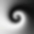
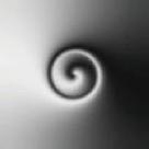
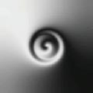
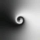
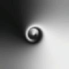
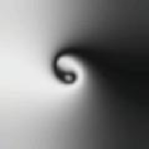
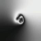
Figure 11: Instability of a rotating spiral. Simulation for a two-dimensional system of size $120\times 120$ with parameters $\omega=2,\alpha=3,\beta=1,K=0.4,l=10,$ and $\tau=10$. Subsequent snapshots of the field Re($\eta$) at times $T$ = 2.8, 10.0, 15.2, 37.2, 96.8, 119.6, 130.0, and 139.2 are presented.

Re$(\eta)$
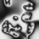
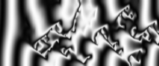
$|\eta|$
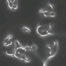
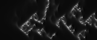
$|z|$

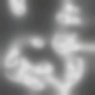
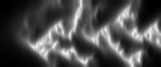
Figure 12: Bursts of desynchronization in a two-dimensional system of size $120\times 120;$ continuation of the simulation presented in Fig. 11. The parameters are $\omega=2,\alpha=3,\beta=1,K=0.4,l=10,$ and $\tau=10$; $T=720$

Typical snapshots of spatial distributions of the variables Re$(\eta)$, $|\eta|$ and $|z|$ in this pattern are displayed in the left panels in Fig. 12. Inside the domains, the coupling field $z$ is reduced in magnitude and these small spatial regions are filled with irregular rapid variations of the complex field $\eta$. Thus, they can be classified as desynchronization bursts. The space-time diagrams through one horizontal cross section of the medium (right panels in Fig. 12) show that such domains can spread or shrink, and travel through the medium. The edges of these structures are marked by the appearance of amplitude defects where $|\eta|$ is close to zero.

Remarkably, if we keep fixed all other parameter values, but eliminate diffusional coupling between the oscillators (the Laplacian term in equation (1a)), evolution starting from the same initial conditions leads to spiral waves with phase-randomized cores, similar to those which were previously considered [15, 14]. Thus, the inclusion of diffusive coupling has a strong effect on pattern formation in the system. Though patterns resembling spiral waves with phase-randomized core are indeed initially developing in the diffusively coupled case, they are unstable and, after a transient, lead to the development of intermittent spatiotemporal regimes with desynchronization bursts.

6 Discussion

Our study can be viewed as an extension of a series of detailed investigations of systems with nonlocal coupling between oscillators performed by Y. Kuramoto with his coworkers. We have chosen the model (1), which belongs to the previously discussed class, and focused our analysis on the effects of coupling inertiality and diffusion in this model. The principal effect of the inertiality in nonlocal coupling is that the system becomes birhythmic and has uniform slow and rapid oscillations as two different coexisting attractors.

For rapid oscillations, the inertial field $z$ responsible for nonlocal coupling is not excited and the system is essentially reduced to an array of only diffusively coupled oscillators with amplitudes $\eta$. In contrast to this, the nonlocal coupling field $z$ is involved in slow oscillations and nonlocal coupling between oscillators is in operation under these conditions.

Our stability analysis based on the phase dynamics equation has shown that, though slow uniform oscillations are always stable in the considered model, rapid uniform oscillations may become modulationally unstable near the birhythmicity boundary. Traveling fronts, separating spatial regions with two different oscillation modes, have been seen in our numerical simulations. Note that the fronts separating oscillating and non-oscillating regions have been recently observed in the vicinity of a subcritical Hopf bifurcation [24].

Irregular intermittent spatiotemporal regimes of two different kinds have been numerically observed. In the patterns with synchronization bursts, the background is occupied by rapid chaotic oscillations. On this background, short-living small domains with slow and rather uniform oscillations spontaneously develop. Inside such domains, the nonlocal coupling field is much larger in magnitude than for the rapidly oscillating background. The characteristic size of such domains was comparable to the nonlocality radius in the model. This kind of intermittent turbulence is to some extent similar to the behavior observed for a system near the Andronov homoclinic bifurcation, exhibiting bistability between a stationary and an oscillatory state [22, 23]. However, the developing domains are filled here not by a stationary state, but by slow oscillations.

In the spatiotemporal patterns with desynchronization bursts, the background is occupied by slow oscillations which are almost uniform. On this background, a cascade of desynchronization bursts develops. Each burst represents a localized turbulent spot filled with rapid irregular oscillations. Inside it, the nonlocal coupling field is reduced in magnitude. Such patterns correspond to the regimes of intermittent localized turbulence previously seen for the complex Ginzburg-Landau equation with global coupling [18], in the experiments with global delayed feedback in surface chemical reactions [26] and in the respective realistic simulations [27]. In some cases, they develop in the situations when rotating spiral waves with phase-randomized cores have been seen [15, 14] in systems where only nonlocal coupling was present. Birhythmicity as a cause of weak turbulence has recently been investigated in a biological model of glycolitic oscillations [25].

Stimulating discussions with Prof. Y. Kuramoto are gratefully acknowledged. We thank M. Stich for the discussion of questions related to birhythmicity.

Appendix A

Starting from system (8) we linearize the first three equations around the values $\rho_{0},r_{0},\psi_{0}$ of the uniform oscillations. The system that we obtain can be written as

$$\dot{\delta\rho} = a_{1}\delta\rho+b_{1}\delta r+c_{1}\delta\psi+d_{1}\nabla\Theta^{2}+e_{1}\nabla^{2}\Theta$$ (11a)

$$\dot{\delta r} = a_{2}\delta\rho+b_{2}\delta r+c_{2}\delta\psi+d_{2}\nabla\Theta^{2}$$ (11b)

$$\dot{\delta\psi} = a_{3}\delta\rho+b_{3}\delta r+c_{3}\delta\psi+d_{3}\nabla\Theta^{2}+e_{3}\nabla^{2}\Theta$$ (11c)

$$\dot{\Theta} = a_{4}\delta\rho+b_{4}\delta r+c_{4}\delta\psi+d_{4}\nabla\Theta^{2}+e_{4}\nabla^{2}\Theta+f_{4}$$ (11d)

where the coefficients are given in the following table

$a_{1}=1-3\rho_{0}^{2}-K$	$a_{3}=2\alpha\rho_{0}+\left[\frac{Kr_{0}}{\rho_{0}^{2}}-r_{0}\frac{1}{\tau}\right]\sin(\psi_{0})$
$b_{1}=K\cos(\psi_{0})$	$b_{3}=\sin(\psi_{0})\left[-\frac{K}{\rho_{0}}+\frac{\rho_{0}}{\tau r_{0}^{2}}\right]$
$c_{1}=-Kr_{0}\sin(\psi_{0})$	$c_{3}=\cos(\psi_{0})\left[-K\frac{r_{0}}{\rho_{0}}+\frac{\rho_{0}}{\tau r_{0}}\right]$
$d_{1}=-\frac{\rho_{0}}{4}$	$d_{3}=-l^{2}\frac{r_{0}}{4\tau}$
$e_{1}=\frac{\zeta}{2}\rho_{0}\beta$	$e_{3}=\frac{1}{2}\left(1-\frac{l^{2}}{\tau}\right)$
$a_{2}=\frac{1}{\tau}\cos(\psi_{0})$	$a_{4}=2\alpha\rho_{0}+\left[K\frac{r_{0}}{\rho_{0}^{2}}+\frac{1}{\tau\rho_{0}}\right]\sin(\psi_{0})$
$b_{2}=-\frac{1}{\tau}$	$b_{4}=\sin(\psi_{0})\left[-\frac{K}{\rho_{0}}-\frac{\rho_{0}}{\tau r_{0}^{2}}\right]$
$c_{2}=-\frac{\rho_{0}}{\tau}\sin(\psi_{0})$	$c_{4}=\cos(\psi_{0})\left[-K\frac{r_{0}}{\rho_{0}}+\frac{\rho_{0}}{\tau r_{0}}\right]$
$d_{2}=-l^{2}\frac{r_{0}}{4\tau}$	$d_{4}=\frac{\beta}{4}$
$e_{2}=0$	$e_{4}=\frac{1}{2}\left(1+\frac{l^{2}}{\tau}\right)$
$f_{4}=-\omega+\alpha\rho_{0}^{2}+\left[-K\frac{r_{0}}{R_{0}}+\frac{\rho_{0}}{\tau r_{0}}\right]\sin(\psi_{0})$

Now, since we are in the approximation where $\rho,r,\psi$ adjust adiabatically to $\Theta$, we can assume $\dot{\delta\rho}=\dot{\delta r}=\dot{\delta\psi}=0$, so that we get from (11d)

$$\delta\rho = \frac{b_{3}c_{2}d_{1}-b_{2}c_{3}d_{1}-b_{3}c_{1}d_{2}+b_{1}c_{3}d_{2}+b_{2}c_{1}d_{3}-b_{1}c_{2}d_{3}}{-a_{3}b_{2}c_{1}+a_{2}b_{3}c_{1}+a_{3}b_{1}c_{2}-a_{1}b_{3}c_{2}+a_{2}b_{1}c_{3}-a_{1}b_{2}c_{3}}\nabla\Theta^{2}$$ (12)

$$+\frac{b_{3}c_{2}e_{1}-b_{2}c_{3}e_{1}+b_{2}c_{1}e_{3}-b_{1}c_{2}e_{3}}{-a_{3}b_{2}c_{1}+a_{2}b_{3}c_{1}+a_{3}b_{1}c_{2}-a_{1}b_{3}c_{2}+a_{2}b_{1}c_{3}-a_{1}b_{2}c_{3}}\nabla^{2}\Theta$$

$$\delta r = \frac{a_{3}c_{2}d_{1}-a_{2}c_{3}d_{1}-a_{3}c_{1}d_{2}+a_{1}c_{3}d_{2}+a_{2}c_{1}d_{3}-a_{1}c_{2}d_{3}}{a_{3}b_{2}c_{1}-a_{2}b_{3}c_{1}-a_{3}b_{1}c_{2}+a_{1}b_{3}c_{2}+a_{2}b_{1}c_{3}-a_{1}b_{2}c_{3}}\nabla\Theta^{2}$$ (13)

$$+\frac{a_{3}c_{2}e_{1}-a_{2}c_{3}e_{1}+a_{2}c_{1}e_{3}-a_{1}c_{2}e_{3}}{a_{3}b_{2}c_{1}-a_{2}b_{3}c_{1}-a_{3}b_{1}c_{2}+a_{1}b_{3}c_{2}+a_{2}b_{1}c_{3}-a_{1}b_{2}c_{3}}\nabla^{2}\Theta$$

$$\delta\psi = \frac{a_{3}b_{2}d_{1}-a_{2}b_{3}d_{1}-a_{3}b_{1}d_{2}+a_{1}b_{3}d_{2}+a_{2}b_{1}d_{3}-a_{1}b_{2}d_{3}}{-a_{3}b_{2}c_{1}+a_{2}b_{3}c_{1}+a_{3}b_{1}c_{2}-a_{1}b_{3}c_{2}-a_{2}b_{1}c_{3}+a_{1}b_{2}c_{3}}\nabla\Theta^{2}$$ (14)

$$+\frac{a_{3}b_{2}e_{1}-a_{2}b_{3}e_{1}+a_{2}b_{1}e_{3}-a_{1}b_{2}e_{3}}{-a_{3}b_{2}c_{1}+a_{2}b_{3}c_{1}+a_{3}b_{1}c_{2}-a_{1}b_{3}c_{2}-a_{2}b_{1}c_{3}+a_{1}b_{2}c_{3}}\nabla^{2}\Theta.$$

These expressions can be put into the equation for $\Theta$ to get

$$\dot{\Theta}=C_{0}+C_{1}(\nabla\Theta)^{2}+C_{2}\nabla^{2}\Theta$$ (15)

where

$$C_{0} = f_{4}$$ (16)

$$C_{1} = d_{4}+\left[c_{4}(a_{3}b_{2}d_{1}-a_{2}b_{3}d_{1}-a_{3}b_{1}d_{2}+a_{1}b_{3}d_{2}+a_{2}b_{1}d_{3}-a_{1}b_{2}d_{3})\right.$$ (17)

$$-b_{4}(a_{3}c_{2}d_{1}-a_{2}c_{3}d_{1}-a_{3}c_{1}d_{2}+a_{1}c_{3}d_{2}+a_{2}c_{1}d_{3}-a_{1}c_{2}d_{3})$$

$$\left.+a_{4}(b_{3}c_{2}d_{1}-b_{2}c_{3}d_{1}-b_{3}c_{1}d_{2}+b_{1}c_{3}d_{2}+b_{2}c_{1}d_{3}-b_{1}c_{2}d_{3})\right]/$$

$$(-a_{3}b_{2}c_{1}+a_{2}b_{3}c_{1}+a_{3}b_{1}c_{2}-a_{1}b_{3}c_{2}-a_{2}b_{1}c_{3}+a_{1}b_{2}c_{3})$$

$$C_{2} = e_{4}+\left[c_{4}(a_{3}b_{2}e_{1}-a_{2}b_{3}e_{1}+a_{2}b_{1}e_{3}-a_{1}b_{2}e_{3})\right.$$ (18)

$$-b_{4}(a_{3}c_{2}e_{1}-a_{2}c_{3}e_{1}+a_{2}c_{1}e_{3}-a_{1}c_{2}e_{3})$$

$$\left.+a_{4}(b_{3}c_{2}e_{1}-b_{2}c_{3}e_{1}+b_{2}c_{1}e_{3}-b_{1}c_{2}e_{3})\right]/$$

$$(-a_{3}b_{2}c_{1}+a_{2}b_{3}c_{1}+a_{3}b_{1}c_{2}-a_{1}b_{3}c_{2}-a_{2}b_{1}c_{3}+a_{1}b_{2}c_{3})$$

References

- [1] Y. Kuramoto, Chemical Oscillations, Waves and Turbulence, (Springer, New York, 1984).
- [2] A. T. Winfree, J. Theor. Biol. 16 (1967) 15.
- [3] R. Imbihl and G. Ertl, Chem. Rev. 95 (1995) 697.
- [4] G. Veser, F. Mertens, A. S. Mikhailov, and R. Imbihl, Phys. Rev. Lett. 71 (1993) 935-939.
- [5] A. S. Mikhailov and B. Hess, J. Phys. Chem. 100 (1996) 19059–19065.
- [6] Y. Kuramoto, Prog. of Theor. Phys. 94 (1995) 321–330.
- [7] Y. Kuramoto and H. Nakao, Phys. Rev. Lett. 76 (1996) 4352–4355.
- [8] Y. Kuramoto and H. Nakao, Physica D 103 (1997) 294–313.
- [9] Y. Kuramoto, D. Battogtokh and H. Nakao, Phys. Rev. Lett.81 (1998) 3543–3546
- [10] D. Battogtokh, Prog. of Theor. Phys. 102 (1999) 947–952.
- [11] Y. Kuramoto, H. Nakao and D. Battogtokh, Physica A 288 (2000) 244–264.
- [12] D. Battogtokh and Y. Kuramoto, Phys. Rev. E 61 (2000) 3227–3230.
- [13] D. Battogtokh, Phys. Lett. A 299 (2002) 558–564.
- [14] Y. Kuramoto, in Nonlinear Dynamics and Chaos: Where do we go from here?, edited by S.J. Hogan, A.R. Champneys, B. Krauskopf, M.d. Bernardo, R.E. Wilson, H.M. Osinga, and M.E. Homer (Institute of Physics, Bristol, 2002) Chapter: Reduction methods applied to nonlocally coupled oscillator systems 800–819.
- [15] S. Shima and Y. Kuramoto, Phys. Rev. E 69 (2004) 036213.
- [16] D. Tanaka and Y. Kuramoto, Phys. Rev. E 68 (2003) 026219.
- [17] D. Battogtokh and A.S. Mikhailov, Physica D 90 (1996) 84.
- [18] D. Battogtokh, A.S. Mikhailov, and A. Preusser Physica D 106 (1997) 327.
- [19] Y. Kawamura and Y. Kuramoto, Phys. Rev. E 69 (2004) 016202.
- [20] M. Stich, M. Ipsen and A. Mikhailov, Phys. Rev. Lett. 86 (2001) 4406.
- [21] M. Stich, M. Ipsen and A. Mikhailov, Physica D 171 (2002) 19.
- [22] M. Argentina and P. Coullet, Phys. Rev. E 56 (1997) R2359-R2362.
- [23] M. Argentina and P. Coullet, Physica A 257 (1998) 45–60.
- [24] P. Coullet and L. Kramer, Chaos 14 (2004) 244.
- [25] D. Battogtokh and J.J. Tyson, Phys. Rev. E 70 (2004) 026212.
- [26] M. Kim, M. Bertram, M. Pollmann, A. von Oertzen, A.S. Mikhailov, H.H. Rotermund, and G. Ertl, Science 292 (2001) 1357.
- [27] M. Bertram and A. S. Mikhailov, Phys. Rev. E 67 (2003) 036207.
- [28] M. Bertram, C. Beta, M. Pollmann, A. S. Mikhailov, H. H. Rotermund, and G. Ertl, Phys. Rev. E 67 (2003) 036208.