Energy Gradient Theory of Hydrodynamic Instability

Abstract

A new universal theory for flow instability and turbulent transition is proposed in this study. Flow instability and turbulence transition have been challenging subjects for fluid dynamics for a century. The critical condition of turbulent transition from theory and experiments differs largely from each other for Poiseuille flows. This enigma has not been clarified so far owing to the difficulty of the problem. In this paper, a new mechanism of flow instability and turbulence transition is presented for parallel shear flows and the energy gradient theory of hydrodynamic instability is proposed. It is stated that the total energy gradient in the transverse direction and that in the streamwise direction of the main flow dominate the disturbance amplification or decay. Thus, they determine the critical condition of instability initiation and flow transition under given initial disturbance. A new dimensionless parameter $K$ for characterizing flow instability is proposed for wall bounded shear flows, which is expressed as the ratio of the energy gradients in the two directions. It is thought that flow instability should first occur at the position of $K_{\max}$ which may be the most dangerous position. This speculation is confirmed by Nishioka et al’s experimental data. Comparison with experimental data for plane Poiseuille flow and pipe Poiseuille flow indicates that the proposed idea is really valid. It is found that the turbulence transition takes place at a critical value of $K_{\max}$ of about $385$ for both plane Poiseuille flow and pipe Poiseuille flow, below which no turbulence will occur regardless the disturbance. More studies show that the theory is also valid for plane Couette flows and Taylor-Couette flows between concentric rotating cylinders. It is concluded that the energy gradient theory is a universal theory for the flow instability and turbulent transition which is valid for both pressure and shear driven flows in both parallel flow and rotating flow configurations.

Keywords: Instability; Transition; Turbulence; Energy gradient; Viscous friction.

1 Introduction

Understanding the mechanism of turbulence has been a great challenge for over a century. Now, it is still very far from approaching a comprehensive theory and the final resolution of the turbulent problem [1]. Reynolds (1883)[1] [2] did the first famous experiments on pipe flow demonstrating the transition from laminar to turbulent flows. Since then, various stability theories emerged during the past 120 years for this phenomenon, but few are satisfactory in the explanation of the various flow instabilities and the related complex flow phenomena.

The pipe Poiseuille flow (Hagen-Poiseuille) is linearly stable for all the Reynolds number $Re$ by eigenvalue analysis [3] [4] [5] [6] [7]. However, experiments showed  that the flow would become turbulence if $Re$ ($=\rho UD/\mu$) exceeds a value of $2000$. Experiments also showed that disturbances in a laminar flow could be carefully avoided or considerably reduced, the onset of turbulence was delayed to Reynolds numbers up to $Re=O(10^{5})$ [6] [7]. For $Re$ above $2000$, the characteristic of turbulence transition depends on the disturbance amplitude and frequency, below which transition from laminar to turbulent state does not occur regardless of the initial disturbance amplitude [8] [9]. Thus, it is clear that the transition from laminar to turbulence for $Re>2000$ is dominated by the behaviours of mean flow and disturbance. Only the combined effect of the two factors reaches the critical condition, could the transition occur for $Re>2000$. These are summarized in Table 1.

Linear stability analysis of plane parallel flows gives critical Reynolds number $Re$ ($=\rho V_{0}h/\mu$) of $5772$ for plane Poiseuille flow, while experiments show that transition to turbulence occurs at Reynolds number of order $1000$ [10] [3] [6] [7], even though the laminar flow could also kept to $Re=O(10^{5})$ [11]. One resolution of these paradoxes is that the domain of attraction for the laminar state shrinks for large Re (as $\mathop{\mathrm{R}e}^{\gamma}$ say, with $\gamma<0),$ so that small but finite perturbations lead to transition [6] [12]. Grossmann [7] commented that this discrepancy demonstrates that nature of the onset-of-turbulence mechanism in this flow must be different from an eigenvalue instability. Orszag and Patera [13] remarked that the mechanism of transition is not properly represented by parallel-flow linear stability analysis. They proposed a linear three-dimensional mechanism to predict the transitional Reynolds number. Some nonlinear stability theories have been proposed, for example, in [14]. However, these theories do not seem to offer a good agreement with the experimental data.

Energy method was also used in the study of flow instabilities [15] [16] [17] [4] [18] [5]. In energy method, one observes the rate of increasing of disturbance energy to study the instability of the flow system. The critical condition is determined by the maximum Reynolds number at which the disturbance energy in the system monotonically decreases. In the flow system, it is considered that turbulence shear stress interacts with the velocity gradient and the disturbance gets energy from mean flow in such a way. Thus, the disturbance is amplified and the instability occurs with the energy increasing of disturbance. Therefore, it is recognized that it is the basic state vorticity leading to instability. The energy method could not get agreement with the experiments either [16] [4] [5]. In recent years, various transition scenarios have been proposed [6] [7] [19] [20] [21] [22] [12] [23] for the subcritical transition. Although we can get a better understanding of the transition process from these scenarios, the mechanism is still not fully understood and the agreement with the experimental data is still not satisfied.

Generally, the transition from laminar flow to turbulent flow is not generated suddenly in the entire flow field but it first starts from somewhere in the flow field and then spreads out gradually from this position. As is well known in solid mechanics, the damage of a metal component generally starts from some area such as manufacturing fault, crack, stress concentration, or fatigue position, etc. In fluid mechanics, we consider that the breaking down of a steady laminar flow should also start from a most dangerous position first. The consequent questions are: (a) Where is this most dangerous position for Poiseuille flow? (b) What is the mechanism and the dominant factor for this phenomenon? (c) What parameter should be used to characterize this position? These questions are our concern. Finding the solution of these problems is important to the understanding of the phenomenon and the estimation of flow transition. Because the turbulence transition is generally resulted in by flow instability [15], we think that the critical condition of transition should be determined by the position where the flow instability first takes place. If the mechanism of flow instability is sought out and the most dangerous position is found, the critical condition of transition could be determined.

Base flow	Disturbance	Resulting flow state
$Re<2000$	No matter how large.	Disturbance decay; flow keeps laminar.
$Re\thicksim 10^{5}$	Kept low.	Flow keeps laminar.
$Re\geq 2000$	Enough large, depend on $Re$.	Transition occurs.

Table 1: Characteristic of transition of Hagen-Poiseuille flow (pipe Poiseuille flow).

In this study, we explore the critical condition of main flow for instability and turbulence transition, and not deal with the detailed process of disturbance amplification. The energy gradient theory is proposed to explain the mechanism of flow instability and turbulence transition for parallel flows. A new dimensionless parameter for characterizing the critical condition of flow instability is proposed. Comparison with experimental data for plane Poiseuille flow and pipe Poiseuille flow at subcritical transition indicates that the proposed idea is really valid.

2 Proposed Mechanism of Flow Instability

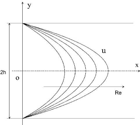
Figure 1: Velocity distribution variation with the increased Reynolds number for given fluid and geometry in plane Poiseuille flows. $Re=\rho UL/\mu,$ $L=2h,$ where $h$ is the half-width of the channel.

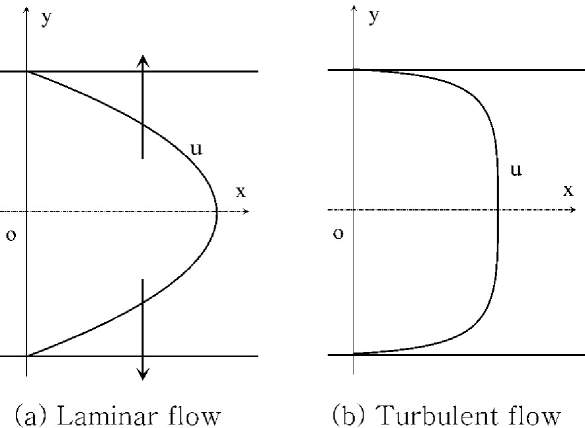
Figure 2: Velocity profiles for laminar and turbulent flows.

The plane Poiseuille flow in a channel is shown in Fig.1. For the given flow geometry and fluid property, with the increasing mean velocity $U$, the flow may transit to turbulence if the $Re$ exceeds a critical value (under certain disturbance). The velocity profiles for laminar and turbulent flows are shown respectively in Fig.2. It can be imagined that there is a “driving factor” which pulls the laminar velocity profile outward toward the walls when the transition takes place. What should be such a driving factor? From a large amount of observations, it is thought that the increase of the gradient of fluid kinematic energy in transverse direction, $\frac{\partial}{\partial y}(\frac{1}{2}V^{2})=V\frac{\partial V}{\partial y}$, may form a “driving force” to cause the increase of flow disturbance for given flow condition, while the gradient of the viscous friction force may resist or absorb the disturbance. Here, $V$ is the magnitude of local velocity. The stability of the flow depends upon the effects of these two roles. With the increasing of mean velocity $U$ for parallel flows, the energy gradient in the transverse direction increases. If this energy gradient is large enough it will lead to a disturbance amplification of the flow. The viscosity friction caused by shear stress would stabilize the flow by absorbing the velocity fluctuation. When the energy gradient in transverse direction reaches beyond a critical value, the laminar flow could not balance this disturbance and flow instability might be excited. Finally, the turbulence flow would be triggered when the transverse energy gradient continuously keeps large enough with the flow forward. The energy gradient in the transverse direction makes the exchange of energy between the fluid layers and sustains the turbulence. Therefore, it is proposed that the necessary condition for the turbulence transition is that there is an energy gradient in the transverse direction of the main flow.

Now, we prove this necessary condition is correct at least for parallel flows. If the gravitational energy is neglected, the total energy gradient in transverse direction is $\frac{\partial}{\partial y}\left(p+\frac{1}{2}\rho V^{2}\right)$. For parallel flows, $\frac{\partial p}{\partial y}=0$ and $V=u$. If this energy gradient is zero, $\frac{\partial}{\partial y}(\frac{1}{2}V^{2})=V\frac{\partial V}{\partial y}=0$, there must be $\frac{\partial V}{\partial y}=0$ due to $V\neq 0$. Thus, the rate of increase of disturbance energy will be negative due to viscous dissipation because the disturbance could not obtain energy from the base flow owing to zero velocity gradient [16] [4] [5]. Therefore, the disturbance must decay at this case. In such way, it is proved that the energy gradient in the transverse direction is a necessary condition for the flow transition.

In addition, when there is a pressure gradient in the normal direction to the flow direction, this pressure gradient could also result in a flow instability even the Reynolds number is low. Both centrifugal and Coriolis instabilities are those caused by pressure gradients. Elastic instability is also that produced by the transversal pressure gradient [25] [26]. The mechanism of instability should take into account of the effect of the variation of cross-streamline pressure for these cases, which may lead to flow instability or accelerates the instability initiation. In some cases of incompressible flows such as stratified flows, the gravitational energy should be taken into account.

For given flow geometry and fluid, it is proposed that the flow stability condition can be expressed as,

$$\frac{\partial}{\partial y}\left(\rho g_{y}y+p+\frac{1}{2}\rho V^{2}\right)<C\text{,}$$ (1)

where $g_{y}$ is the component of gravity acceleration in $y$ direction, and $C$ is a constant which is related to fluid property and geometry. The $x$ axis is along the flow direction and the $y$ axis is along the transverse direction. In this study, we first show that the proposed idea is really correct for Poiseuille flows.

3 Formulation and Theory Description

The conservation of momentum for an incompressible Newtonian fluid is (neglecting gravity force):

$$\rho(\frac{\partial\mathbf{V}}{\partial t}+\mathbf{V}\cdot\nabla\mathbf{V})=-\nabla p+\mu\nabla^{2}\mathbf{V}\text{.}$$ (2)

Using the identity,

$$\mathbf{V}\cdot\nabla\mathbf{V}=\frac{1}{2}\nabla\left(\mathbf{V}\cdot\mathbf{V}\right)-\mathbf{V}\times\nabla\times\mathbf{V}\text{,}$$ (3)

equation (2) can be rearranged as,

$$\rho\frac{\partial\mathbf{V}}{\partial t}+\nabla(p+\frac{1}{2}\rho V^{2})=\mu\nabla^{2}\mathbf{V}+\rho\mathbf{(V}\times\nabla\times\mathbf{V)}\text{,}$$ (4)

where $\rho$ is the fluid density, $t$ the time, $\mathbf{V}$ the velocity vector, $p$ the hydrodynamic pressure, $\mu$ the dynamic viscosity of the fluid. If the viscous force is zero, the above equation becomes the Lamb form of momentum equation. This equation can be found in most text books. For incompressible flow, the total pressure represents the total energy in Eq. (4). Actually, the energy equation has long been used for stability analysis as previously mentioned [18] [4] [5] [17] [16].

In previous sections, it is proposed that the instability of viscous flows depends on the relative magnitude of the energy gradient in transverse direction and the viscous friction term. A larger energy gradient in transverse direction tries to lead to amplification of a disturbance, and a large shear stress gradient in streamwise direction tends to absorb this disturbance and to keep the original laminar flow state. The transition of turbulence depends on the relative magnitude of the two roles of energy gradient amplification and viscous friction damping under given disturbance. We propose the parameter for characterizing the relative role of these effects below.

Let $d\mathbf{s}$ represent the differential length along a streamline in a Cartesian coordinate system,

$$d\mathbf{s}=d\mathbf{x}+d\mathbf{y}\text{.}$$ (5)

With dot multiplying Eq. (4) by $d\mathbf{s}$, we obtain,

$$\rho\frac{\partial\mathbf{V}}{\partial t}\cdot d\mathbf{s}+\nabla(p+\frac{1}{2}\rho V^{2})\cdot d\mathbf{s}=\mu\nabla^{2}\mathbf{V}\cdot d\mathbf{s}+\rho\mathbf{(V}\times\nabla\times\mathbf{V)}\cdot d\mathbf{s}\text{.}$$ (6)

Since $\mathbf{(V}\times\nabla\times\mathbf{V)}\cdot d\mathbf{s=}0$ along the streamline, for steady flows, we obtain the energy gradient along the streamline,

$$\partial(p+\frac{1}{2}\rho V^{2})/\partial s=\mu\nabla^{2}\mathbf{V}\cdot\frac{d\mathbf{s}}{\left|d\mathbf{s}\right|}\mathbf{=}(\mu\nabla^{2}\mathbf{V)}_{s}\text{.}$$ (7)

This equation shows that the total energy gradient along the streamwise direction equals to the viscous term $(\mu\nabla^{2}\mathbf{V)}_{s}$. For pressure driving flows, $(\mu\nabla^{2}\mathbf{V)}_{s}$ represents the energy loss due to friction. It is obvious that the total energy decreases along the streamwise direction due to viscous friction loss. The energy gradient along the transverse direction is,

$$\partial(p+\frac{1}{2}\rho V^{2})/\partial n=\frac{\partial p}{\partial n}+\rho V\frac{\partial V}{\partial n}\text{.}$$ (8)

It can be seen that the energy gradient at transverse direction depends on the velocity gradient and the velocity magnitude as well as the transversal pressure gradient.

The relative magnitude of the energy gradients in the two directions can be expressed by a new dimensionless parameter, $K,$ the ratio of the energy gradient in the transverse direction to that in the streamwise direction,

$$K=\frac{\partial E/\partial n}{\partial E/\partial s}=\frac{\partial(p+\frac{1}{2}\rho V^{2})/\partial n}{\partial(p+\frac{1}{2}\rho V^{2})/\partial s}=\frac{\partial p/\partial n+\rho V(\partial V/\partial n)}{(\mu\nabla^{2}\mathbf{V)}_{s}}\text{,}$$ (9)

where $E=p+\frac{1}{2}\rho V^{2}$ expresses the total energy, $n$ denotes the direction normal to the streamwise direction, and $s$ denotes the streamwise direction.

It is noticed that the parameter $K$ is a field variable and it represents the direction of the vector of local total energy gradient. It can be seen that when $K$ is small, the role of the viscous term in Eq.(9) is large and the flow tends to be stable. When $K$ is large, the role of numerator in Eq.(9) is large and the flow tends to be unstable. For given flow field, there is a maximum of $K$ in the domain which represents the most possible unstable location. Therefore, in the area of high value of $K$, the flow tends to be more unstable than that in the area of low value of $K$. The first instability should be initiated by the maximum of $K$, $K_{max}$, in the flow field for given disturbance. In other words, the position of maximum of $K$ is the most dangerous position. The magnitude of $K_{max}$ in the flow field symbolizes the extent of the flow approaching the instability. Especially, if $K_{max}=\infty$, the flow is certainly potential to be unstable under some disturbance. For given flow disturbance, there is a critical value of $K_{max}$ over which the flow becomes unstable. In particular, corresponding to the subcritical transition in wall bounded parallel flows, the $K_{max}$ reaches its critical value, below which no transition occurs regardless of the disturbance amplitude.  For unidirectional parallel flows, this critical value of $K_{max}$ should be a constant regardless of the fluid property and the magnitude of the geometrical parameter. Now, owing to the complexity of the flow, it is difficult to predict this critical value by theory. Nevertheless, it can be determined by the experimental data for given flows.

For parallel flows, the coordinates $s-n$ becomes the $x-y$ coordinates and the pressure gradient $\partial p/\partial n=\partial p/\partial y=0$. Thus, using the global approximation, $\partial(\frac{1}{2}\rho V^{2})/\partial y\backsim\rho U^{2}/L$, $\left(\mu\nabla^{2}\mathbf{V}\right)_{s}\backsim\partial^{2}u/\partial y^{2}\backsim U/L^{2}$, we obtain $K\backsim$ $\rho UL/\mu=Re,$ where $L$ is a characteristic length in the transverse direction. Thus, the parameter $K$ is equivalent to the Reynolds number in the global sense for parallel flows.

The negative energy gradient in the streamwise direction plays a part of resisting on or absorbing the disturbance. Therefore, it has a stable role to the flow. The energy gradient in the transverse direction has a role of amplifying disturbance. Therefore, it has a unstable role to the flow. Here, it is not to say that a high energy gradient in transverse direction necessarily leads to instability, but it has a potential for instability. Whether instability occurs also depends on the magnitude of the disturbance. From this discussion, it is easily understood that the disturbance amplitude required for instability is small for high energy gradient in transverse direction (high Re) [9].

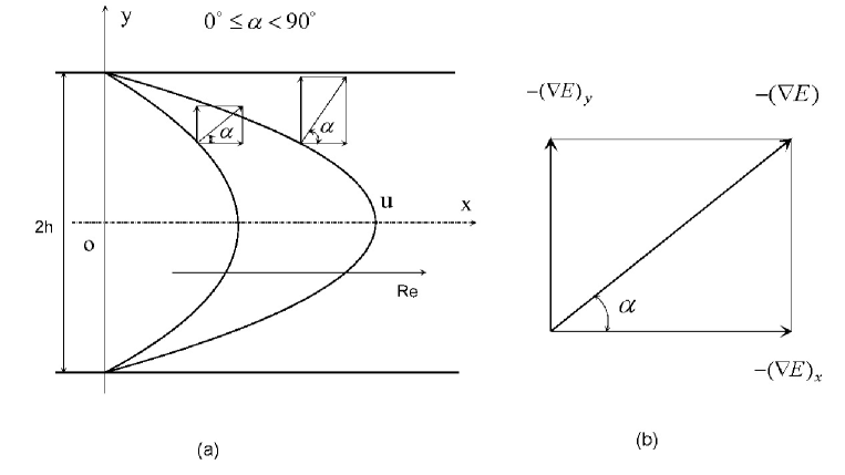
Figure 3: Schematic of energy gradient and energy angle for plane Poiseuille flows. (a) Energy angle increases with the Reynolds number; (b) Definition of the energy angle.

Figure 4: Schematic of the direction of the total energy gradient and energy angle for flow with an inflection point at which the energy angle equals 90 degree.

The value of “$\arctan K$” expresses the angle between the direction of the total energy gradient and the streamwise direction. We write that,

$$\alpha=\arctan K\text{.}$$ (10)

In this paper, the angle $\alpha$ is named as “energy angle,” as shown in Fig.3. The value of the energy angle (its absolute value) can also be used to express the extent of the flow near the instability occurrence. Fig.3 and Fig.4 show the schematic of the energy angle for some flows. There is a critical value of energy angle, $\alpha_{c},$ corresponding to the critical value of $K_{max}$. When $\alpha>\alpha_{c}$,  the flow becomes unstable. For Poiseuille flows, $0^{\circ}\leq\alpha<90^{\circ}$ and the stability depends on the magnitudes of the energy angle and the disturbance. For parallel flow with a velocity inflection, $\alpha=90^{\circ}$ ($K_{max}=\infty$) at the inflection point and the flow is therefore unstable. This is for the first time to theoretically prove that viscous flow with a velocity inflection is unstable. Inversely, as discussed before, viscous flow without velocity inflection may not be necessarily stable, depending on the flow conditions (as shown in table 1). These results are correct at least for pressure driving flows.

Fig.4 is a best explanation of inflectional instability for viscous flows. According to Eq.(9), the physics of the criterion presented in this paper is easily understood. The energy gradient in the transverse direction tries to amplify a small disturbance, while the energy loss due to friction in the streamwise direction plays a damping part to the disturbance. The parameter $K$ represents the relative magnitude of disturbance amplification due to energy gradient and disturbance damping of viscous loss. When there is no inflection point in the velocity distribution, the amplification or decay of disturbance depends on the two roles above, i.e., the value of $K.$ When there is an inflection point in the velocity distribution, the viscous term vanishes, and while the transversal energy gradient still exists at the position of inflection point. Thus, even a small disturbance must be amplified by the energy gradient at this location. Therefore, the flow will be unstable. Rayleigh (1880) [24] only proved that inviscid flow with an inflection point is unstable, while we demonstrate here that viscous flow with an inflection point is unstable. The Rayleigh’s criterion was derived from mathematics using the inviscid theory, but its physical meaning is still not clear.

It is well known that viscosity plays dual role on the flow instability and disturbance amplification [4] [18] [5] [15]. It can be seen from equation (9) that the higher the viscosity, the larger the viscous friction loss. Thus, the flow is more stable. If the values of the vorticity and the streamwise velocity are high, the transversal energy gradient will be high. Thus, the flow is more unstable. From these discussion, it is known that viscosity mainly plays a stable role to the initiation of flow instability at subcritical transition by affecting the base flow through the viscous friction of streamwise velocity. This is consistent with criterion of the Reynolds number.

Reynolds number represents the ratio of convective inertia force to the viscous force in the Navier-Stokes equations as a dimensionless parameter. However, the magnitude of the Reynolds number is only a global indication of the flow states and a rough expression for the transition condition. At same $Re$ number, the behaviour of flow instability may be different due to the different combination of the magnitude of viscosity with other parameters when $Re$ is larger than an indifference Reynolds number, as shown by the chart of the solution of the Orr-Sommerfeld equation [18] [27] [28]. The role of viscosity is complicated with the variations of flow parameters and flow conditions. The generation of turbulence is not simply caused by increasing the $Re$, but actually by increasing the value of $K$. When $Re$ increases, it inevitably leads to the increase of $K$ in the flow field. The magnitude of local disturbance for a fixed point depends not only on the apparent $Re$ number, but also on the local flow conditions. For steady Poiseuille flow, the convective inertia term is zero and the flow becomes turbulent at high $Re$. We can see that the occurrence of turbulence is not due to the convective inertia term in this case. In Poiseuille flow, the local Reynolds number is high in the core area along the centerline, but the degree of turbulence is low. In the area near the wall, the local Reynolds number is low, but the degree of turbulence is high. In uniform flows, high Reynolds number may not necessarily leads to turbulence. In summary, the Reynolds number is only a global parameter, and the $K$ is a local parameter which represents the local behaviour of the flow and best reflects the role of energy gradient.

4 Analysis on Poiseuille Flows

4.1 Plane Poiseuille Flow

Figure 5: Kinematic energy gradient and viscous force term versus the axial pressure gradient for plane Poiseuille flow for any position in the flow field. $\left|dp/dx\right|\propto U\propto Re$ for given fluid and geometry.

The instability in Poiseuille flows with increasing mean velocity $U$ can be demonstrated as below for a given fluid and flow geometry by using the energy gradient concept.

For 2D Poiseuille flow, the momentum equation is written as,

$$0=-\rho\frac{\partial p}{\partial x}+\mu\frac{\partial^{2}u}{\partial y^{2}}\text{,}$$ (11)

showing that viscous force term is proportional to the streamwise pressure gradient. The integration to above equation gives,

$$u=u_{0}\left(1-\frac{y^{2}}{h^{2}}\right)\text{,}$$ (12)

where $u_{0}=-\frac{1}{2\mu}h^{2}\frac{\partial p}{\partial x}$, is the centerline velocity, and $h$ is the channel half width.

Although the energy gradient is not explicitly shown in above equation, it can be expressed as below for any position in the flow field (noticing $v=0$),

$$\frac{\partial}{\partial y}\left(\frac{1}{2}\rho V^{2}\right)=-\frac{\rho}{2\mu^{2}}h^{2}y\left(1-\frac{y^{2}}{h^{2}}\right)\left(\frac{\partial p}{\partial x}\right)^{2}\text{.}$$ (13)

Thus, for any position in the flow field,

$$\left|\frac{\partial}{\partial y}\left(\frac{1}{2}\rho V^{2}\right)\right|\propto\left|\left(\frac{\partial p}{\partial x}\right)^{2}\right|\text{.}$$ (14)

The behaviours of the equations (11–14) are shown in Fig.5:  the viscous force term is linear, while the kinematic energy gradient increases quadratically with the pressure gradient. Therefore, at low value of mean velocity $U$, the viscous friction term could balance the disturbance amplification caused by energy gradient. At large value of $U$, the viscous friction term may not constrain the disturbance amplification caused by energy gradient and the flow may transit to turbulence.

For plane Poiseuille flows, the ratio of the energy gradient to the viscous force term, $K$, is ($\partial p/\partial y=0$),

$$K = \frac{\partial}{\partial y}\left(\frac{1}{2}\rho V^{2}\right)/\left(\mu\frac{\partial^{2}u}{\partial y^{2}}\right)=-\frac{2\rho yu_{0}}{h^{2}}u_{0}\left(1-\frac{y^{2}}{h^{2}}\right)/\left(-\mu\frac{2u_{0}}{h^{2}}\right)$$ (15)

$$= \frac{3}{2}\frac{\rho Uh}{\mu}\frac{y}{h}\left(1-\frac{y^{2}}{h^{2}}\right)=\frac{3}{4}Re\frac{y}{h}\left(1-\frac{y^{2}}{h^{2}}\right)\text{.}$$

Here, $Re=\rho UL/\mu$, and $U=\frac{2}{3}u_{0}$ has been used for plane Poiseuille flow. $u_{0}$ is the maximum velocity at centerline and $U$ is the averaged velocity. It can be seen that $K$ is proportional to $Re$ for a fixed point in the flow field.

The distribution of $u,E,$ and $K$ along the transversal direction for plane Poiseuille flow is shown in Fig.6. It is clear that there are maximum of $K$ at ${y/h=\pm 0.5774}$, as shown in Fig.6. This maximum can also be obtained by differentiating the equation (15) with $y/h$ and letting the derivatives equal to zero. Since we concern the maginitude of the $K$ and the velocity profile is symmetrical to the centerline, we refer the maximum of $K$ as its positive value thereafter. We think that the flow breakdown of the Poiseuille flow should not suddenly occur in the entire flow field, but it first takes place at the location of $K_{\max}$ in the domain, then it spreads out according to the distribution of $K$ value. The formation of turbulence spot in shear flows may be related to this procedure.

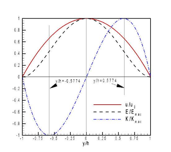
Figure 6: Velocity, energy, and $K$ along the transversal direction $y/h$ for plane Poiseuille flow, which are normalized by the their maximum.

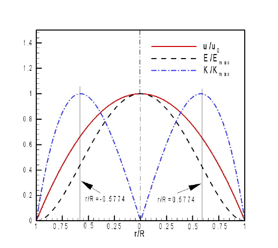
Figure 7: Velocity, energy, and $K$ along the transversal direction $r/R$ for pipe Poiseuille flow, which are normalized by the their maximum.

4.2 Pipe Poiseuille Flow

Similar analysis to the plane Poiseuille flow can be carried out for the circular Poiseuille flow. For circular pipe Poiseuille flow, the momentum equation is written as,

$$0=-\rho\frac{\partial p}{\partial z}+\mu\left(\frac{\partial^{2}u_{z}}{\partial r^{2}}+\frac{1}{r}\frac{\partial u_{z}}{\partial r}\right)\text{,}$$ (16)

showing that viscous force term is also proportional to the streamwise pressure gradient. The axial velocity is expressed as by integration on above equation,

$$u_{z}=u_{0}\left(1-\frac{r^{2}}{R^{2}}\right)\text{,}$$ (17)

where $u_{0}=-\frac{1}{4\mu}R^{2}\frac{\partial p}{\partial z}$, is the centerline velocity, $z$ is in axial direction and $r$ is in radial direction of the cylindrical coordinates, and $R$ is the radius of the pipe. The energy gradient can be expressed as below for any position in the flow field (noticing $u_{r}=0$),

$$\frac{\partial}{\partial r}\left(\frac{1}{2}\rho V^{2}\right)=-\frac{\rho}{8\mu^{2}}R^{2}r\left(1-\frac{r^{2}}{R^{2}}\right)\left(\frac{\partial p}{\partial z}\right)^{2}\text{.}$$ (18)

Similar to plane Poiseuille flow, the viscous force term is linear, while the kinematic energy gradient increases quadratically with the pressure gradient.

For pipe Poiseuille flows, the ratio of the energy gradient to the viscous force term, $K$, is ($\partial p/\partial r=0$),

$$K = \frac{\partial}{\partial r}\left(\frac{1}{2}\rho V^{2}\right)/\mu\left(\frac{\partial^{2}u_{z}}{\partial r^{2}}+\frac{1}{r}\frac{\partial u_{z}}{\partial r}\right)=-\frac{2\rho ru_{0}}{R^{2}}u_{0}\left(1-\frac{r^{2}}{R^{2}}\right)/\left(-\mu\frac{4u_{0}}{R^{2}}\right)$$ (19)

$$= \frac{\rho UR}{\mu}\frac{r}{R}\left(1-\frac{r^{2}}{R^{2}}\right)=\frac{1}{2}Re\frac{r}{R}\left(1-\frac{r^{2}}{R^{2}}\right)\text{.}$$

Here, $Re=\rho UD/\mu$, and $U=\frac{1}{2}u_{0}$ has been used for pipe Poiseuille flow. $u_{0}$ is the maximum velocity at centerline and $U$ is the averaged velocity.

The distribution of $K$ along the transversal direction for pipe Poiseuille flow is the same as that for plane Poiseuille flow if it is normalized by its maximum and $y/h$ is replaced by $r/R$, and the maximum of $K$ also occurs at ${r/R=0.5774}$, as shown in Fig.7.

5 Comparison with Experiments

Flow type	Authors	$Re_{c}$	$Re_{c}$
Poiseuille pipe			$Re=\rho UD/\mu$
	Reynolds (1883)		$2300$
	Petal & Head (1969)		$2000$
	Darbyshire & Mullin(1995)		$1760\thicksim 2300$
	Most literature cited		$2000$
Poiseuille plane		$Re=\rho UL/\mu$	$Re=\rho u_{0}h/\mu$
	Davies & White (1928)	$1440$	$1080$
	Patel & Head (1969)	$1350$	$1012$
	Carlson et al (1982)	$1340$	$1005$
	Alavyoon et al (1986)	$1466$	$1100$
	Most literature cited		$1000$

Table 2: Collected experimental data of the critical Reynolds number for plane Poiseuille flow and pipe Poiseuille flow. U is the averaged velocity. $u_{0}$=2U, and D is the diameter of the pipe for pipe Poiseuille flow. $u_{0}$=1.5U, L =2h, and L is the hight of the channel for plane Poiseuille flow.

Experiments for Poiseuille flows indicated that when the Reynolds number is below a critical value, the flow is laminar regardless of the disturbances. For circular Poiseuille flow (Hagen-Poiseuille), Reynolds (1883) [2] carried out the first systematic experiment on the flow transition and found that the critical Reynolds number for transition to turbulence is about $Re_{c}=\rho UD/\mu=2300$, where the $U$ is the averaged velocity and $D$ is the diameter of the pipe. Now, the most accepted critical value is $Re_{c}=\rho UD/\mu=2000$ which is demonstrated by numerous experiments [28]. All the collected data could be put in a range of $1760$ to $2300$ [9]. There are also experimental data for the transition for plane Poiseuille flows in the literature. Davies and White [29] showed that the critical Reynolds number for transition to turbulence is $Re_{c}=\rho UL/\mu=1440$ for plane Poiseuille flow, where the $U$ is the averaged velocity and $L=2h$ is the width of the channel. Patel and Head [30] obtained a critical value for turbulence transition, $Re_{c}=2000$ for pipe Poiseuille flow, and $Re_{c}=1350$ for channel flow through detailed measurements. Carlson et al. [31] found the transition at about $Re_{c}=1340$ for plane Poiseuille flow using flow visualization technique. Alavyoon et al.’s [32] experiments show that the transition to turbulence for plane Poiseuille flow occurs around $Re_{c}=\rho u_{0}h/\mu=1100$. The most accepted value of minimum $Re_{c}$ for plane Poiseuille flow is about $Re_{c}=\rho u_{0}h/\mu\thickapprox 1000$ [6] [7]. All the collected experimental data are listed in Table 2. Although these experiments are done at various different environmental conditions, they are all near a common accepted value of critical Reynolds number. In the following, we show that there is a critical value of $K_{\max}$ at which the flow becomes turbulent. In order to more exactly compare plane Poiseuille flow to pipe Poiseuille flow at same experimental conditions, we prefer here to use Patel and Head’s data [30] to evaluate the parameters at the critical conditions. Patel and Head’s data are also the best to fit all of the data and are cited by most literature.

Now, we calculate the critical value of $K_{\max}$ at the transition condition for both plane Poiseuille flow and pipe Poiseuille flow using Eqs.(15) and (19), respectively. For plane Poiseuille flow,  one obtains $K_{\max}{=389}$ at the critical Reynolds number ${Re}_{c}{=1350}$. For pipe Poiseuille flow, one obtains $K_{\max}{=385}$ at the critical Reynolds number ${Re}_{c}{=2000}$. These results are shown in Table 3. In this table, the critical Reynolds number obtained from energy method is also listed. From the comparison of critical values of $K_{\max}$ for plane Poiseuille flow and pipe Poiseuille flow, we find that although the critical Reynolds number is different for the two flows, the turbulence transition takes place at the same $K_{\max}$ value, about $385\backsim 389$. This demonstrated that $K_{\max}$ is really a dominating parameter for the transition, and $K_{\max}$ is a better expression than the $Re$ number for the transition condition. We can further conclude that energy gradient theory is better than the linear stability theory for the prediction of critical Reynolds number of subcritical transition. In this way, the proposed idea is verified for wall bounded parallel shear flows. Therefore, it may be presumed that the transition of turbulence in other complicated shear flows would also depend on the $K_{\max}$ in the flow field.

Flow type	$Re$ expression	Eigenvalue analysis	Energy	Experiments	$K_{\max}$ at Exp
		$Re_{c}$	method $Re_{c}$	$Re_{c}$	$Re_{c}$ value
Poiseuille pipe	$Re=\rho UD/\mu$	stable for all $Re$[7]	81.5	$2000$[30]	$385$
Poiseuille plane	$Re=\rho UL/\mu$	$7696$[10]	68.7	$1350$[30]	$389$
	$Re=\rho u_{0}h/\mu$	$5772$[10]	49.6	$1012$[30]	$389$
Plane Couette	$Re=\rho u_{h}h/\mu$	stable for all $Re$[7]	20.7	$370$[37, 38]	$370$

Table 3: Comparison of the critical Reynolds number and the ratio of the energy gradient to the viscous force term, $K_{\max}$ for plane Poiseuille flow and pipe Poiseuille flow. The critical Reynolds number by energy method is taken from Schmid and Henningson (2001).

Nishioka et al (1975)’s famous experiments [11] for plane Poiseuille flow showed details of the outline and process of the flow breakdown. The measured instantaneous velocity distributions suggest that the break down of the flow is a local phenomenon, at least in its initial stage. As in Fig.8, the base flow is laminar and the instantaneous distribution of the velocity breaks at the position $y/h=0.50$ ($T=4$ to $6$) to $0.62$ ($T=8$ to $9$) by showing an oscillation of velocity in $y/h=0.50\thicksim 0.62$. They show an inflectional velocity in this range of $y/h$. This result means that the flow breakdown first occurs in the range of $y/h=0.50\thicksim 0.62$. This coincides to the prediction of our theory, i.e., the position of $K_{\max}$ is the most dangerous point which occurs at $y/h=0.5774$. These results are enough to confirm the theory of “energy gradient” valid at least for Poiseuille flows (pressure driving flow).

For pipe flow, in a recent study [33], Wedin and Kerswell showed that there is the presence of the “shoulder” in the velocity profile at about $r/R=0.6$ from their solution of travelling waves. They suggested that this corresponds to where the fast streaks of traveling waves reach from the wall. It can be construed that this kind of velocity profile as obtained by simulation is similar to that of Nishioka et al’s experiments for channel flows. The location of the “shoulder” is about same as that for $K_{\max}$. According to the present theory, this “shoulder” may then be intricately related to the distribution of energy gradient. The solution of traveling waves has been confirmed by experiments more recently [34].

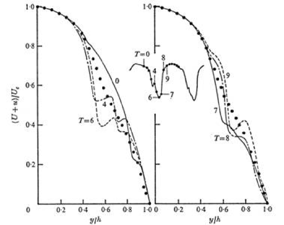
Figure 8: Instantaneous velocity distributions in a plane Poiseuille flow (Nishioka et al. 1975) [11]. Time T corresponding to each distribution is noted on the trace of the u fluctuation at y/h=0.6, sketched in the figure. Solid circle is the mean velocity. Uc is the velocity on the channel center-plane. y/h=0 is at the center-plane and y/h=1 is at the wall. Instantaneous velocity U+u at a point is composed of the mean velocity U and the fluctuation velocity u. (Courtesy of Nishioka; Use permission by Cambridge University Press).

The energy gradient theory can also be used to explain the reason why it is not appropriate to scale the outer flow or overlap profiles of channel flow and those of pipe flow at the same Reynolds number turbulent flows[35].  This is easily understood by the fact that pipe Poiseuille flow has a same velocity and energy gradient distributions in the radial direction as the plane Poiseuille flow has in the $y$ direction, but the former has a smaller hydraulic diameter than the latter and has more viscous friction. Therefore, the scaling should be carried out at the same $K_{\max}$ value, but not at the same Reynolds number (Fig.8).  At a same Reynolds number, for example, say, $1000$, the plane Poiseuille flow reaches the critical $Re$ number for transition, while pipe Poiseuille flow is far from the critical $Re$ number, as shown in Fig.9a. The flow state at these two flows are definitely different at this Re number. This principle also applies to turbulence flow range. If we compare the two type of flows at same $K_{\max}$ value, they should have the same flow behaviour (Fig.9b).

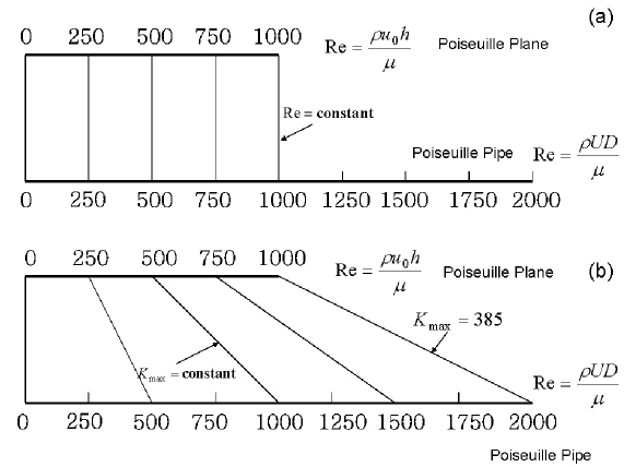
Figure 9: Scaling of plane Poiseuille flow with pipe Poiseuille flow. (a) Keeping the $Re$ is constant. (b) Keeping the $K_{\max}$ is constant.   The correlation should be carried out at the same $K_{\max}$ vaue (b), rather at the same Re (a).

In a separating paper [36] (owing to the space limit here), we apply the energy gradient theory to the shear driving flows, and show that this theory is also correct for plane Couette flow. We obtain $K_{\max}=370$ at the critical transition condition determined by experiments below which no turbulence occurs (see Table 3). This value is near the value for Poiseuille flows, $385\backsim 389$. The minute difference in the number is not important because there is some difference in the determination of the critical condition. For example, the judgement of transition is from the chart of drag coefficient in Patel and Head [30], while visualization method is used in [37, 38]. These results demonstrate that the critical value of $K_{\max}$ at subcritical transition for wall bounded parallel flows including both pressure driven and shear driven flows is about $370\backsim 389$.

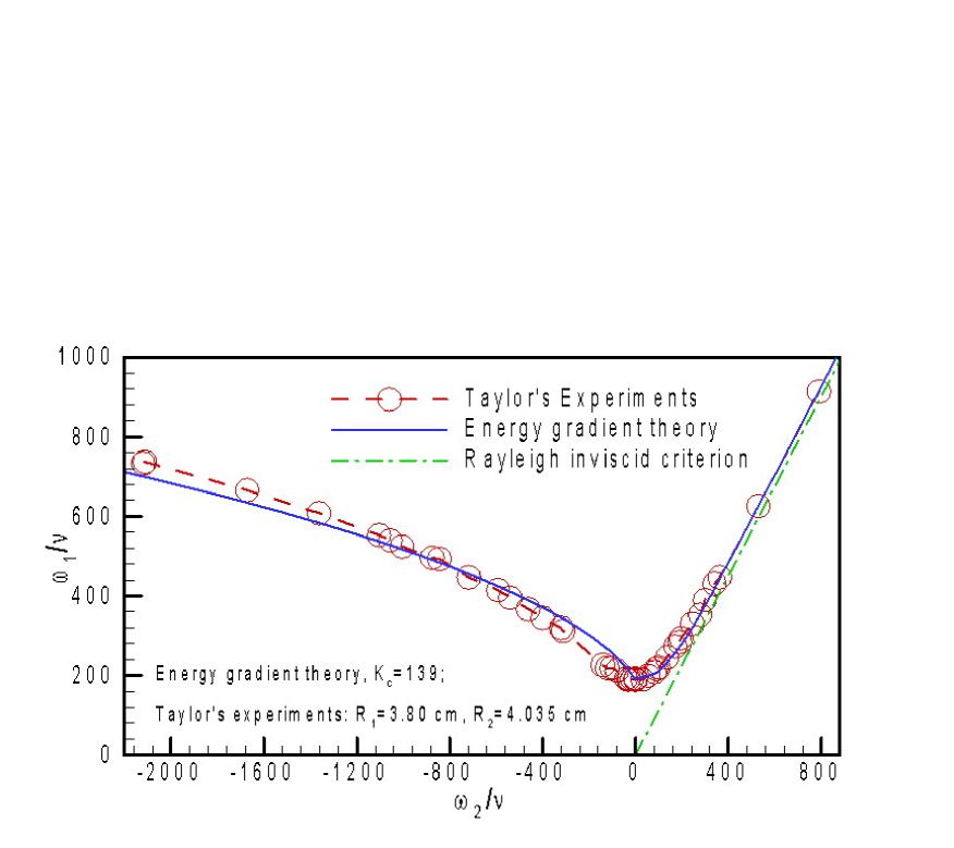
Figure 10: Comparison of the theory with the experimental data for the instability condition of Taylor-Couette flow between concentric rotating cylinders ($R_{1}$=3.80cm, $R_{2}$=4.035 cm). $R_{1}$: radius of the inner cylinder; $R_{2}$: radius of the outer cylinder. $\omega_{1}$ and $\omega_{2}$ are the angular velocities of the inner and outer cylinders, respectively. The critical value of the energy gradient parameter Kc=139 is determined by the experimental data at $\omega_{2}=0$ and $\omega_{1}\neq 0$ (the outer cylinder is fixed, the inner cylinder is rotating). With $K_{c}$=139, the critical value of $\omega_{1}/\nu$ versus $\omega_{2}/\nu$ is calculated using the energy gradient thoery for $\omega_{2}/\nu$ = -2200—900 [39].

More recently, the energy gradient theory is applied to the Taylor-Couette flow between concentric rotating cylinders [39]. The detailed derivation for the calculation of the energy gradient parameter is provided in the study. The theoretical results for the critical condition of primary instability obtain very good agreement with Taylor’s experiments (1923) [40] and others, see Fig.10. Taylor (1923) used mathematical theory and linear stability analysis and showed that linear theory obtained agreement with the experiments. However, as is well know and discussed before, linear theory is failed for wall bounded parallel flows. As shown in this paper, the present theory is valid for all of these said flows. Therefore, it is concluded that the energy gradient theory is a universal theory for the flow instability and turbulent transition which is valid for both pressure and shear driven flows in both parallel flow and rotating flow configurations.

The Rayleigh-Benard convective instability and the stratified flow instability could also be considered as being produced by the energy gradient transverse to the flow (thermal or gravitational energy). The energy gradient theory can be not only used to predict the generation of turbulence, but also it may be applied to the area of catastrophic event predictions, such as weather forecast, earthquakes, landslides, mountain coast, snow avalanche, motion of mantle, and movement of sand piles in desert, etc. The breakdown of these mechanical systems can be universally described in detail using this theory. In a material system, when the maximum of energy gradient in some direction is greater than a critical value for given material properties, the system will be unstable. If there is a disturbance input to this system, the energy gradient may amplify the disturbance and lead to the system breakdown. This problem will be further addressed in future study.

6 Conclusions

The mechanism for the flow instability and turbulent transition in parallel shear flows is studied in this paper. The energy gradient theory is proposed for the flow instability. The theory is applied to plane channel flow and Hagen-Poiseuille flow. The main conclusions of this study are as follows:

1. A mechanism of flow instability and turbulence transition is presented for parallel shear flows. The theory of energy gradient is proposed to explain the mechanism of flow instability and turbulence transition. It is stated that the energy gradient in transverse direction tries to amplify the small disturbance, while viscous friction in streamwise direction could resist or absorb this small disturbance. Initiation of instability depends upon the two roles for given initial disturbance. Viscosity mainly plays a stable role to the initiation of flow instability by affecting the base flow.

2. A universal criterion for the flow instability initiation has been formulated for wall shear flows. A new dimensionless parameter characterizing the flow instability, $K$, which is defined as the ratio of the energy gradients in transverse direction and that in streamwise direction, is proposed for wall bounded shear flows. The most dangerous position in the flow field can be represented by the maximum of $K$. The initiation of flow breakdown should take place at this position first. This idea is confirmed by Nishioka et al.’s experiments.

3. The concept of energy angle is proposed for flow instability. This concept helps to understand the mechanism of viscous instabilities. Using the concept of energy gradient and energy angle, it is theoretically demonstrated for the first time that viscous flow with a velocity inflection is unstable.

4. It is demonstrated that there is a critical value of the parameter $K_{\max}$ at which the flow transits to turbulence for both plane Poiseuille flow and pipe Poiseuille flow, below which no turbulence exists. This value is about $K_{\max}{=385\backsim 389}$. Although the critical Reynolds number is different for the two flows, the turbulence transition takes place at the same $K_{\max}$ value.

5. The energy gradient theory is a universal theory for the flow instability and turbulent transition which is valid for both pressure and shear driven flows in both parallel flow and rotating flow configurations.

Acknowledgment

The author would like to thank Professors N Phan-Thien (National University of Singapore) and JM Floryan (University of West Ontario) for their comments on the first version of the manuscript.

References

- [1] J.L.Lumley and A.M. Yaglom, A Century of Turbulence, Flow, Turbulence and Combustion, 66, 241-286 (2001).
- [2] O. Reynolds, An experimental investigation of the circumstances which determine whether the motion of water shall be direct or sinuous, and of the law of resistance in parallel channels, Phil. Trans. Roy. Soc. London A, 174, 935-982 (1883).
- [3] L.D.Landau and E.M.Lifshitz, Fluid Mechanics, 2nd Ed., (Pergamon, Oxford, 1987), pp.95-191.
- [4] P.G.Drazin and W.H.Reid, Hydrodynamic Stability, (Cambridge University Press, Cambridge, 1981), pp.1-250.
- [5] P.J.Schmid, and D.S.Henningson, Stability and transition in shear flows, (Springer, New York, 2001).
- [6] L.N.Trefethen, A.E. Trefethen, S.C.Reddy, T.A.Driscoll, Hydrodynamic stability without eigenvalues, Science, 261, 578-584 (1993).
- [7] S.Grossmann, The onset of shear flow turbulence. Reviews of modern physics, 72, 603-618 (2000).
- [8] I.J.Wygnanski, and F.H. Champagne, On transition in a pipe. Part 1. The origin of puffs and slugs and the flow in a turbulent slug. J. Fluid Mech. 59, 281-335 (1973).
- [9] A.G.Darbyshire and T.Mullin, Transition to turbulence in constant-mass-flux pipe flow, J. Fluid Mech, 289, 83-114 (1995).
- [10] S.A.Orszag, Accurate solution of the Orr-Sommerfeld stability equation, J. Fluid Mech, 50, 689-703 (1971).
- [11] M. Nishioka, S Iida, and Y.Ichikawa, An experimental investigation of the stability of plane Poiseuille flow, J. Fluid Mech, 72, 731-751 (1975).
- [12] S.J. Chapman, Subcritical transition in channel flows, J. Fluid Mech, 451, 35-97 (2002).
- [13] S.A.Orszag and A.T. Patera, Subcritical transition to turbulence in plane channel flows, Physical review letters, 45(1980) 989-993.
- [14] J.T.Stuart, Nonlinear Stability Theory, Annual Review of Fluid Mechanics, 3, 347-370 (1971).
- [15] C.-C. Lin, The Theory of Hydrodynamic Stability, Cambridge Press,1955. Cambridge,1-153.
- [16] R.Betchov, and W.O.Criminale,Jr., Stability of parallel flows, Academic Press,New York,1967, 168-170.
- [17] D.D.Joseph, Stability of fluid motions, Vol.1 and 2, Berlin : Springer-Verlag , 1976.
- [18] J.O.Hinze, Turbulence, 2nd Ed., (McGraw-Hill, New York, 1975), pp.586-770.
- [19] F.Waleffe, Transition in shear flows, nonlinear normality versus nonnormal linearity, Phys. Fluids, 7, 3060–3066 (1995).
- [20] J.S.Baggett, and L.N.Trefethen, Low-dimensionalmodes of subcritical transition to turbulence, Phys. Fluids, 9, 1043-1053 (1997).
- [21] O.Y.Zikanov, On the instability of pipe Poiseuille flow, Phys. Fluids, 8, 2923-2932 (1996).
- [22] S.C. Reddy, P.J. Schmid, J.S.Baggett, and D.S. Henningson, On stability of streamwise streaks and transition thresholds in plane channel flows, J. Fluid Mech, 365, 269-303 (1998).
- [23] A.Meseguer, Streak breakdown instability in pipe Poiseuille flow, Phys. Fluids, 15, 1203-1213 (2003).
- [24] L. Rayleigh, On the stability or instability of certain fluid motions, Proc. Lond. Maths. Soc. 11 57-70 (1880).
- [25] E.S.G.Shaqfeh, Purely elastic instabilities in viscoelastic flows, Annual Review of Fluid Mechanics, 28, 129-186 (1996).
- [26] H.-S.Dou and N. Phan-Thien, Numerical simulation of viscoelastic flows past a linear array of cylinders by parallel compuation, Computational Fluid Dynamics 2002, S.Armfield, P.Morgan, and K. Srinivas Eds., (Springer, Berlin, 2002),323-328.
- [27] F.M. White, Viscous Fluid Flow. (McGraw-Hill, New York, 2nd Ed., 1991).
- [28] H.Schlichting and K.Gersten, Boundary Layer Theory, (Springer, 8th Ed., Berlin, 2000), pp.415-494.
- [29] S.J.Davies and C.M.White, An experimental study of the flow of water in pipes of rectangular section, Proc. Roy. Soc. A, 119, 92-107 (1928).
- [30] V.C.Patel, and M.R.Head, Some observations on skin friction and velocity profiles in full developed pipe and channel flows, J. Fluid Mech, 38, 181-201 (1969).
- [31] D.R.Carlson, S.E.Widnall, M.F.Peeters, A flow-visualization study of transition in plane Poiseuille flow, J. Fluid Mech, 121, 487-505 (1982).
- [32] F.Alavyoon, D.S.Henningson, P.H.Alfredsson, Turbulent spots in plane Poiseuille flow–flow visualization, Phys. Fluids, 29, 1328-1331 (1986).
- [33] H. Wedin, and R.R. Kerswell, Exact coherent structures in pipe flow: travelling wave solutions, J. Fluid Mech. 508, 333-371 (2004).
- [34] B. Hof, C.W. H. van Doorne, J.Westerweel, F.T. M. Nieuwstadt, H.Faisst, B.Eckhardt, H.Wedin, R.R. Kerswell, F.Waleffe, Experimental observation of nonlinear traveling waves in turbulent pipe flow, Science, 305 (2004), Issue 5690, 10 September 2004, 1594-1598.
- [35] M. Wosnik, L. Castill, W.K. George, A theory for turbulent pipe and channel flows, J. Fluid Mech, 421, 115-145 (2000).
- [36] H.-S. Dou, B.C.Khoo, K.S.Yeo, and N.Phan-Thien, Instability of plane couette flow, Technical Report, National University of Singapore, 2003.
- [37] F. Daviaud, J. Hegseth, and P. Berge’, Subcritical transition to turbulence in plane Couette flow, Phys. Rev. Lett. 69, 2511-2514 (1992).
- [38] N. Tillmark and P. H. Alfredsson, Experiments on transition in plane Couette flow, J. Fluid Mech. 235, 89 –102 (1992).
- [39] H.-S. Dou, B.C.Khoo, K.S.Yeo, and N.Phan-Thien, Instability of Taylor-Couette flow between rotating concentric cylinders, submitted to a Journal, Nov., 2004.
- [40] G. I. Taylor, Stability of a Viscous Liquid Contained between Two Rotating Cylinders, Philosophical Transactions of the Royal Society of London. Series A, Vol. 223. (1923), 289-343.