Desynchronized wave patterns in synchronized chaotic regions of coupled map lattices

Abstract

We analyze the size limits of coupled map lattices with diffusive coupling at the crossover of low-dimensional to high-dimensional chaos. We investigate the existence of standing-wave-type periodic patterns, within the low-dimensional limit, in addition to the stable synchronous chaotic states depending upon the initial conditions. Further, we bring out a controlling mechanism to explain the emergence of standing-wave patterns in the coupled map lattices. Finally, we give an analytic expression in terms of the unstable periodic orbits of the isolated map to represent the standing-wave patterns.

I Introduction

Coupled dynamical systems often arise in nature whenever a collective or cooperative phenomenon is favoured Lakshmanan and Murali (1996); Pikovsky et al. (2001); Lakshmanan and Rajasekar (2003); Muruganandam et al. (1999). In particular, the coupled map lattice with diffusive coupling (CML) provides a prototype model to study various features associated with the cooperative evolution of constituent systems Kaneko (1986, 1992); Lind et al. (2002); Francisco and Muruganandam (2003); Kaneko and Tsuda (2000). One of the important properties of such CMLs is that they exhibit size instability, that is, there is a critical size on the number of constituents for which stable synchronous chaotic state exists. Increasing the number of constituents beyond this limit leads to the occurrence of spatially incoherent behaviour (eg., high-dimensional chaos). For example, Bohr and Christensen Bohr and Christensen (1989) have studied such size instability behaviour in a two-dimensional coupled logistic lattice. Similar desynchronization has been found in arrays of coupled systems represented by nonlinear oscillators Muruganandam et al. (1999); Heagy et al. (1994); Pecora and Carroll (1998); Restrepo et al. (2004). The stability of synchronous chaos in coupled dynamical systems plays an important role in the study of pattern formation, spatiotemporal chaos, etc. Muruganandam et al. (1999); Heagy et al. (1994); Bohr and Christensen (1989); Rangarajan and Ding (2002); Chen et al. (2003).

In general, these studies on size instability are valid in most situations. However, we have noted that in certain circumstances there is an ambiguity in dealing with these systems below the critical system sizes. To be specific, there exist certain nontrivial ranges of initial conditions for which the CML admits spatial and temporally periodic solutions in contrast to the usually expected stable synchronous chaos. In this brief report, we show numerically the coexistence of such periodic states with the stable synchronous chaotic state well below the critical system size and explain the underlying mechanism.

II Size instability in Coupled Map Lattices with diffusive coupling

Consider an one-dimensional coupled map lattice with nearest-neighbour diffusive coupling Kaneko (1986, 1992)

$$x_{n+1}^{j}=f(x_{n}^{j})+\epsilon\left[f(x_{n}^{j-1})+f(x_{n}^{j+1})-2f(x_{n}^{j})\right],$$ (1)

where $j$ $(=0,1,2,\cdots,L-1)$ represents the lattice sites and $L$ is the system size, subject to periodic boundary conditions.

The stability analysis of the synchronized chaotic state defined by $s_{n}=x^{0}=x^{1}=\cdots=x^{L-1}$ in the above CML using the procedure derived originally for coupled oscillators by Heagy et al Heagy et al. (1994), gives the relation connecting transverse Lyapunov exponents (TLEs), in terms of the Lyapunov exponent of single (isolated) map, $\lambda^{0}$ as

$$\lambda^{k}=\lambda^{0}+\ln\left[1-4\epsilon\text{sin}^{2}\left(\frac{\pi k}{L}\right)\right].$$ (2)

The synchronous state is stable only if the TLEs ($\lambda^{k}$, $k=1,2,\cdots\,L-1$) are all negative.

The above relation (2) can also be obtained by means of a direct perturbation of the form

$$x_{n}^{j}=s_{n}+\delta\,\exp\left(i\frac{2\pi k}{L}\right)\,\exp\left(\lambda^{k}n\right),\;\;\delta\ll 1,$$ (3)

as considered by Bohr and Christensen Bohr and Christensen (1989).

The synchronous state loses its stability when the long waves (lowest mode) are unstable Bohr and Christensen (1989). This means that for $\lambda^{1}>0$ the synchronous state is unstable. Thus, substituting $\lambda^{1}=0$ in Eq. (2), one obtains the maximum/critical lattice size $(L_{c})$ that supports stable synchronous state as

$$L_{c}=\text{int}\left(\frac{\pi}{\text{sin}^{-1}\left(\sqrt{\frac{1-e^{-\lambda_{0}}}{4\epsilon}}\right)}\right).$$ (4)

Now, let us consider a coupled logistic lattice with diffusive coupling (CLL) where each lattice site in Eq. (1) is occupied by the logistic map

$$f(x)=\mu x(1-x),\;\;x\in(0,1),\;\;\mu\in(0,4).$$ (5)

In particular for the choice $\mu=3.5732$, the Lyapunov exponent of single (isolated) map is positive (i.e., $\lambda^{0}\sim 0.057>0$) and chaotic. In this case, for coupling strength $\epsilon=0.2$, the critical lattice size ($L_{c}$) is found to be $11$ from Eq. (4). That is, upto the lattice size $11$ the CLL exhibits synchronous chaos and for lattice size $\geq 12$ the synchronization is found to be lost, thereby confirming the size instability in the diffusively coupled logistic lattices.

III Existence of Multiple stable states in Coupled Map Lattices

When random initial conditions are assumed, in most cases, the above CLL with diffusive coupling exhibits stable synchronous chaos for $2\leq L\leq 11$ as predicted by Eq. (4). However, there are certain ranges of initial conditions for which CLL shows some interesting asynchronous spatiotemporal patterns even for $L<L_{c}$. For

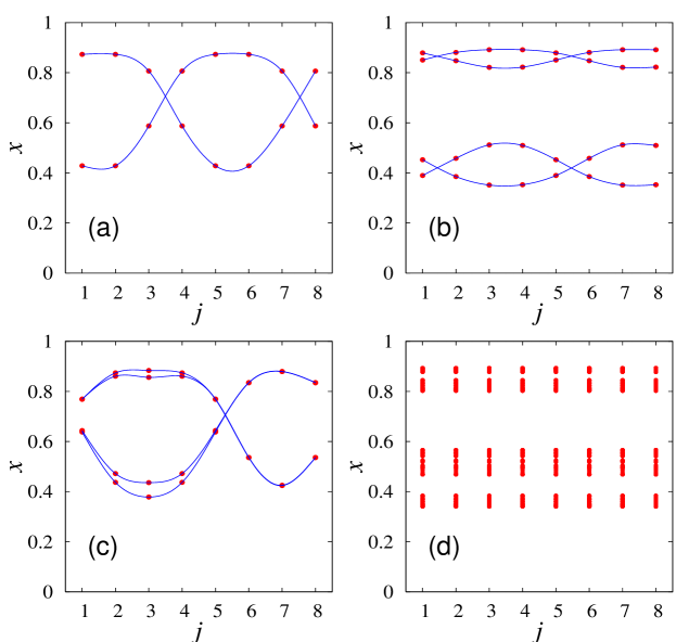
Figure 1: The possible spatiotemporal patterns in coupled logistic lattice (1) and (5) with $L=8$ for different initial conditions. (a) single standing wave, (b) double standing waves (c) single standing wave with a temporal period-2 orbit in one half and period-4 orbit in the other half of the lattice and (d) synchronized chaos.

example, for $L=8$ and with the choice of initial conditions $\{x^{j}_{0}\}_{j=0}^{L-1}=$ $\{0.1$, $0.01$, $0.7$, $0.2$, $0.65$, $0.1$, $0.15$, $0.001\}$ or several nearby initial conditions, the CLL exhibits a standing wave type pattern as shown in Fig. 1(a). But for the same lattice size, if we choose a different set of initial conditions, $\{x^{j}_{0}\}_{j=0}^{L-1}=$ $\{0.0004$, $0.0001$, $0.0003$, $0.0005$, $0.00045$, $0.00018$, $0.00016$, $0.00001\}$ or the nearby points, two standing waves with different amplitudes are produced within the CLL as in Fig. 1(b). Similarly a disturbed standing wave pattern as shown in Fig. 1(c) is possible to be exhibited by the CLL for many choices of initial conditions. A synchronous chaos, as one would expect for $L=8$ from the theory, is also exhibited by the CLL as depicted in Fig. 1(d), for most of the random choices of initial conditions. This kind of multiple stable solutions is also observed in the CLL for other lattice sizes, namely $L=6$, $7$, $9$ and $10$ which are also less than $L_{c}$. The occurrence of various spatiotemporal patterns for different lattice sizes of the CLL and their percentage of occurrence are shown in Table 1. In order to quantify the percentage of occurrence of different spatiotemporal patterns, we have used $10^{6}$ sets of random initial conditions (i.c.’s) in the interval $0$ to $1$ and identified the number of i.c.’s which lead to a specific pattern as indicated in Table 1. We have further confirmed our assertion by analyzing the same systems in different computing environments such as Intel Pentium 4, Sun Sparc server/workstation and Compaq Alpha workstation.

In addition, by considering the whole CML of size $L$ as a single $L$-dimensional map we have verified that the above spatiotemporal periodic structures are essentially the stable fixed points of this map. For example, the periodic structure in Fig. 1(a) represents a fixed of point of period-2 of the eight-dimensional map and the eigenvalues of the corresponding Jacobian matrix all are having magnitude less than unity. In a similar fashion one can verify that all the periodic structures are the stable fixed points of corresponding periods. Thus, in addition to the stable synchronized manifold, there exists other invariant sets corresponding to stable periodic structures.

Table 1: The possible spatiotemporal patterns for different lattice sizes and their percentage of occurrence for the coupled logistic lattice sampled over a set of $10^{6}$ random initial conditions (IC’s). The parameters are fixed as $\mu=3.5732$ in Eq. (5) and $\epsilon=0.2$ in Eq. (1). Here, SW: standing wave, sync.: synchronized.

size	spatiotemporal	% of	size	spatiotemporal	% of
($L$)	patterns	IC’s	($L$)	patterns	IC’s
$6$	single SW	$9$	$10$	double SWs	$43$
	sync. chaos	$91$		sync. chaos	$45$
$7$	single SW	$22$		others	$12$
	sync. chaos	$78$	$11$	double SWs	$48$
$8$	single SW	$21$		four SWs	$2$
	double SWs	$10$		sync. chaos	$34$
	sync. chaos	$66$		others	$16$
	others	$3$	$12$	double SWs	$24$
$9$	double SWs	$38$		four SWs	$28$
	sync. chaos	$54$		sync. chaos	$0.2$
	others	$8$		others	$47.8$

IV Emergence of standing wave patterns by controlling

The extraordinary behaviour of the CML with diffusive coupling showing standing wave patterns well below the critical lattice size ($L_{c}$) can be explained as follows. The second term in the right hand side of Eq. (1), can be considered as a kind of force or perturbation applied to every lattice point in the CML and we call it as the coupling force. In fact this force on a particular lattice point is developed either due to a mismatch in the parameters of the neighbouring lattice points or due to differences in their initial conditions or both. If the neighbouring lattice points are identical then this force is formed due to variation in the initial conditions and our system indeed falls under this category. In general, the strength of the coupling force at all the lattice points approaches zero when they oscillate towards synchronization with their neighbours, and usually this will happen for $L\leq L_{c}$. But in the case of $L>L_{c}$, this force at every lattice point oscillates periodically or in a chaotic manner, giving rise to various spatiotemporal patterns, including standing waves. However, as we have pointed out above that under certain circumstances, (i.e., for certain ranges of initial conditions), even for $L<L_{c}$, the coupling force of each and every lattice point oscillates periodically with different amplitudes and thereby makes the CML to exhibit spatiotemporal periodic (standing wave) solutions. In general, the periodic oscillations in the coupling force may be of any period and this fixes the number of standing waves produced within the lattice.

In order to understand the mechanism behind the emergence of spatiotemporal periodic structure, let us now consider a specific case of the periodically oscillating coupling force of period two, that is, the force oscillating between two fixed amplitudes, say, $k_{1}$ and $k_{2}$ so that a single standing wave is formed in the CML. Then the amplitudes of the coupling force at the $j^{th}$ lattice site will alternate between the numerical values $k^{j}_{1}$ and $k^{j}_{2}$, where $j=1,2,\ldots,L$. Thus, the evolution of $j^{th}$ map in the CML can be effectively described by the equation

$$x^{j}_{n+1}\,=f(x^{j}_{n})+k^{j}_{1},\;\; x^{j}_{n+2}\,=f(x^{j}_{n+1})+k^{j}_{2}.$$ (6)

For a given lattice point $j$, this is nothing but a single logistic map with a periodic kick of period-2 (modified map). It is now obvious to note from Eqs. (6) and (1) that the original coupled map lattice exhibiting a standing wave pattern can be decomposed into $L$ number of modified maps such that the dynamics of (1) is essentially mimicked by the set (6). Thus studying the evolution of $L$ decoupled modified maps (6) with allowed sets of values for $k^{j}_{1}$ and $k^{j}_{2}$ is equivalent to that of the original CML, given by Eq. (1).

In general, a chaotically evolving system can be controlled to a stable periodic orbit by the addition of an appropriate constant or periodic external bias Pyragas (1993); Loskutov and Shismarev (1994); Lakshmanan and Rajasekar (2003); A. Venkatesan, S. Parthasarathy, and M. Lakshmanan (2003); Palaniyandi and Lakshmanan (2005). As a consequence, one can expect a stable fixed point solution for the modified map (6) for appropriate forcing amplitudes ($k_{1}$ and $k_{2}$), with same set of parameters for which the original map, $x^{j}_{n+1}=f(x^{j}_{n})$, exhibits chaotic solution. Thus there exists a possibility for obtaining periodic solutions of period two for the constituent map within the CML even though its parameter is in the chaotic region of the individual map.

In the case of coupled logistic lattice with parameters mentioned in the previous section, the allowed region of forcing amplitudes which lead the decoupled modified map (6) to exhibit period two solution is shown in Fig. 2. For $L=8$, we have calculated the amplitudes of the coupling force [that is, the second term in the right hand side of Eq. (1)] of period-$2$ for the initial conditions, $\{x^{j}_{0}\}_{j=0}^{L-1}=$ $\{0.1$, $0.01$, $0.7$, $0.2$, $0.65$, $0.1$, $0.15$, $0.001\}$, and these are shown in Table 2. Now one can easily check that these amplitudes of the coupling force fall in the region specified by the phase diagram shown in Fig. 2. Also, the shift invariant property of the

Figure 2: The phase diagram in the $k_{1}-k_{2}$ plane for the modified map (6) with $f(x)=\mu x(1-x)$, $\mu=3.5732$, showing the regions which correspond to the periodic solution of period $2$ (dark region).

CLL ensures that there is no temporal variation if we shift the initial conditions of each lattice point in the CML to its neighbour spatially. In this case, the wave pattern will also make only a corresponding shift. We have made similar investigations for higher periodic standing waves which lead to same type of conclusions based on the appropriate periodic nature of the coupling force.

Table 2: Amplitudes of the coupling force $k_{1}$ and $k_{2}$ in the coupled map lattices for $L=8$ with period-$2$ for initial conditions, $\{x^{j}_{0}\}_{j=0}^{L-1}=$ $\{0.1$, $0.01$, $0.7$, $0.2$, $0.65$, $0.1$, $0.15$, $0.001\}$.

lattice	$k_{1}^{j}$	$k_{2}^{j}$	lattice	$k_{1}^{j}$	$k_{2}^{j}$
site(j)	($\times 10^{-2}$)	($\times 10^{-2}$)	site(j)	($\times 10^{-2}$)	($\times 10^{-2}$)
$1$	$-0.17626$	$3.24717$	$5$	$3.24717$	$-0.17626$
$2$	$-5.98282$	$2.91190$	$6$	$2.91190$	$-5.98282$
$3$	$2.91190$	$-5.98282$	$7$	$-5.98282$	$2.91190$
$4$	$3.24717$	$-0.17626$	$8$	$-0.17626$	$3.24717$

So, if it is possible to control the coupling force to fall in the region which corresponds to a periodic solution, then one can obtain standing wave patterns irrespective of the size of the lattices. This is in fact possible by choosing appropriate initial conditions to each lattice point and this explains the occurrence of standing waves (asynchronous) as shown in Figs. 1(a) and 1(b) in the CLL well below the critical lattice size ($L_{c}$). Similar explanation holds good for Fig. 1(c). The same principle is involved in the occurrence of standing waves even for $L>L_{c}$ Kaneko (1992).

V Analytical expression for standing wave patterns

From a careful numerical analysis, we have observed that the nodes and antinodes of standing waves are formed at or very close to the UPOs

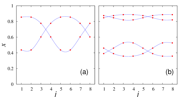
Figure 3: Standing wave patterns obtained from Eq. (7) for $L=8$: (a) standing wave with period-1 UPO at nodes and period-2 UPO at antinodes and (b) period-2 UPO at nodes and period-4 UPO at antinodes.

of the isolated logistic map. Keeping this in mind, we propose an expression for the standing wave pattern Main (1993) of the form

$$x^{j}=u_{k}+A_{k}\sin\left(\frac{m\pi(j-\delta)}{L}\right)\cos\left(\pi i\right),$$ (7)

where,

$$A_{k}=\left\{\begin{array}[]{ll}A^{\mbox{\scriptsize max}}_{k},&\text{~{}~{}~{}if }\sin\left(\frac{m\pi(j-\delta)}{L}\right)\cos\left(\pi i\right)>0\\ A^{\mbox{\scriptsize min}}_{k},&\text{~{}~{}~{}if }\sin\left(\frac{m\pi(j-\delta)}{L}\right)\cos\left(\pi i\right)<0\end{array}\right.$$ (9)

where the discrete index $j=0,1,2,\cdots,L-1$ corresponds to the lattice site, $m$ denotes the mode of the waves, and $k$ and $i$ represent the nodes and antinodes of different standing waves present in the pattern, which can take values from $1$ to $p$ and $1$ to $2p$, respectively and $p$ is the period of UPO. Also in the above equation (7), $u_{k}$’s represent the values of the UPOs of the isolated logistic map at the node of the $k$-th standing wave, and $A^{\mbox{\scriptsize max}}_{k}$ and $A^{\mbox{\scriptsize min}}_{k}$ are the absolute values of the differences between UPOs at the node and UPOs at high and low amplitudes at the antinodes of the $k$th standing waves, respectively. The wave patterns with one and two number of standing waves obtained using Eq. (7) for $L=8$ are shown in Fig. 3, whereas for the same lattice size, the numerically obtained pattern which have been discussed in Sec. III is shown in Figs. 1(a) and 1(b). One observes that these two figures coincide very closely.

VI Summary and Conclusion

In this report, we have pointed out that coupled map lattices with diffusice coupling exhibit multiple stable states for the same set of parameters with respect to the initial conditions. It has also been shown that by choosing appropriate initial conditions, one can obtain different standing wave type patterns for such coupled map lattices even for lattice size much less than the critical system size $L_{c}$, where one normally would expect synchronized chaos. In addition, we have proposed the mechanism behind the occurrence of such standing wave patterns.