Acceleration and vortex filaments in turbulence

Abstract

We report recent results from a high resolution numerical study of fluid particles transported by a fully developed turbulent flow. Single particle trajectories were followed for a time range spanning more than three decades, from less than a tenth of the Kolmogorov time-scale up to one large-eddy turnover time. We present some results concerning acceleration statistics and the statistics of trapping by vortex filaments.

Lagrangian statistics of particles advected by a turbulent velocity field, $\bm{u}(\bm{x},t)$, are important both for their theoretical implications K65 and for applications, such as the development of phenomenological and stochastic models for turbulent mixing pope . Despite recent advances in experimental techniques for measuring Lagrangian turbulent statistics cornell ; pinton ; ott_mann ; leveque , direct numerical simulations (DNS) still offer higher accuracy albeit at a slightly lower Reynolds number yeung ; BS02 ; IK02 . Here, we describe Lagrangian statistics of velocity and acceleration in terms of the multifractal formalism. At variance with other descriptions based on equilibrium statistics (see e.g. beck ; aringazin ; arimitsu , critically reviewed in GK03 ), this approach has the advantage of being founded on solid phenomenological grounds. Hence, we propose a derivation of the Lagrangian statistics directly from the Eulerian statistics.

We analyze Lagrangian data obtained from a recent Direct Numerical Simulation (DNS) of forced homogeneous isotropic turbulence biferale04 ; biferale04b which was performed on $512^{3}$ and $1024^{3}$ cubic lattices with Reynolds numbers up to $R_{\lambda}\sim 280$. The Navier-Stokes equations were integrated using fully de-aliased pseudo-spectral methods for a total time $T\approx T_{L}$. Two millions of Lagrangian particles (passive tracers) were injected into the flow once a statistically stationary velocity field had been obtained. The positions and velocities of the particles were stored at a sampling rate of $0.07\tau_{\eta}$. The velocity of the Lagrangian particles was calculated using linear interpolation. Acceleration was calculated both as the derivative of the particle velocity and by direct computation from all three forces acting on the particle (i.e. pressure gradients, viscous forces and large scale forcing): the two measurements were found to be in very good agreement. Finally, the flow was forced by keeping the total energy constant in each of the first two wavenumber shells. For more details on the simulation, see biferale04 ; biferale04b .

I Velocity and acceleration statistics

Velocity statistics along a particle trajectory can be measured by means of the Lagrangian structure functions, $S_{p}(\tau)=\langle(\delta_{\tau}v)^{p}\rangle$ where $\delta_{\tau}v$ is the Lagrangian increment of one component of the velocity field in a time lag $\tau$. A simple way to link the Lagrangian velocity increment, $\delta_{\tau}v$, to the Eulerian one, $\delta_{r}u$, is to consider the velocity fluctuations along a particle trajectory as the superposition of different contributions from eddies of all sizes. In a time-lag $\tau$ the contributions from eddies smaller than a given scale, $r$, are uncorrelated, and we may write $\delta_{\tau}v\sim\delta_{r}u$. Assuming that typical eddy turn over time $\tau$ at a given spatial scale $r$ can be expressed as $\tau_{r}\sim r/\delta_{r}u$, one obtains:

$$\delta_{\tau}v\sim\delta_{r}u\qquad\tau\sim\frac{L^{h}_{0}}{v_{0}}r^{1-h},$$ (1)

where $h$ is the local scaling exponent characterizing the Eulerian fluctuation in the multifractal phenomenology frisch . Also, $L_{0},v_{0}$ are the integral scale and the typical velocity, respectively. With respect to the the usual multifractal phenomenology of fully developed turbulence, the presence of a fluctuating eddy turn over time is the only extra additional ingredient to take into account in the Lagrangian reference frame.

Using (1), one can estimate the Lagrangian velocity structure function:

$$S_{p}(\tau)\sim\langle v_{0}^{p}\rangle\int_{h\in I}\mbox{d}h\left(\frac{\tau}{T_{L}}\right)^{\frac{hp+3-D(h)}{1-h}},$$ (2)

where the factor $(\tau/T_{L})^{(3-D(h))/(1-h)}$ is the probability of observing an exponent $h$ in a time-lag $\tau$, and $D(h)$ is the dimension of the fractal set where the exponent $h$ is observed. The Lagrangian scaling exponents $\zeta_{L}(p)$ can be estimated by a saddle point approximation, for $\tau\ll T_{L}$:

$$\zeta_{L}(p)=\inf_{h}\left(\frac{hp+3-D(h)}{1-h}\right).$$ (3)

We would like to stress that for the $D(h)$ curve we have chosen that of the Eulerian statistics. In other words, the prediction (3) is free of any additional parameter once the Eulerian statistics are assumed borgas93 ; BDM02 ; biferale04 .

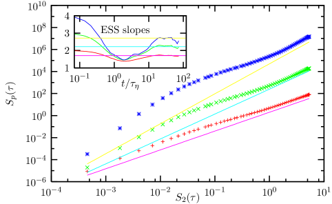
Figure 1: ESS plot of Lagrangian velocity structure function $S_{p}(\tau)$ versus $S_{2}(\tau)$. Symbols refer to the DNS data for $p=8,6,4$ from top to bottom. Lines have slopes $\zeta_{L}(p)/\zeta_{L}(2)$ given by the multifractal prediction (3) with a $D(h)$ curve taken from the She-Leveque prediction she_leveque . In the inset, we show the local slopes versus time $\tau/\tau_{\eta}$, and their comparison with the respective multifractal prediction (straight lines).

In Fig. (1), we present the Extended Self Similarity (ESS) ess log-log plot of $S_{p}(\tau)$ versus $S_{2}(\tau)$ as calculated from our DNS. The logarithmic local slopes shown in the inset display a deterioration of scaling quality for small times. We explain this strong bottleneck for time lags, $\tau\in[\tau_{\eta},10\tau_{\eta}]$, in terms of trapping events inside vortical structures biferale04 : a dynamical effect which may strongly affect scaling properties and which a simple multifractal model cannot capture. For this reason, scaling properties are recovered only using ESS and for large time lags, $\tau>10\tau_{\eta}$. In this interval a satisfactory agreement with the multifractal prediction (3) is observed, namely from the multifractal model one can estimate $\zeta_{L}(4)/\zeta_{L}(2)=1.71,\zeta_{L}(6)/\zeta_{L}(2)=2.26,\zeta_{L}(8)/\zeta_{L}(2)=2.72$ while from our DNS we measured $\zeta_{L}(4)/\zeta_{L}(2)=1.7\pm 0.05,\zeta_{L}(6)/\zeta_{L}(2)=2.2\pm 0.07,\zeta_{L}(8)/\zeta_{L}(2)=2.75\pm 0.1$.

A similar phenomenological argument can be used to make a prediction for the acceleration probability density function (pdf). The acceleration can be defined as:

$$a\equiv\frac{\delta_{\tau_{\eta}}v}{\tau_{\eta}}.$$ (4)

As the Kolmogorov scale itself, $\eta$, fluctuates in the multifractal formalism: $\eta(h,v_{0})\sim\left(\nu L_{0}^{h}/v_{0}\right)^{1/(1+h)},$ so does the Kolmogorov time scale, $\tau_{\eta}(h,v_{0})$. Using (1) and (4) evaluated at $\eta$, we get for a given $h$ and $v_{0}$:

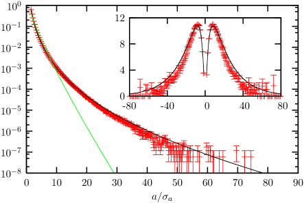
Figure 2: Log-linear plot of the acceleration pdf. The crosses are the DNS data, the solid black line is the multifractal prediction and the green line is the K41 prediction. The statistical uncertainty in the pdf is quantified by assuming that fluctuations grow proportional to the square root of the number of events. Inset: ${\tilde{a}}^{4}{\cal P}({\tilde{a}})$ for the DNS data (crosses) and the multifractal prediction.

$$a(h,v_{0})\sim\nu^{\frac{2h-1}{1+h}}v_{0}^{\frac{3}{1+h}}L_{0}^{-\frac{3h}{1+h}}.$$ (5)

The pdf of the acceleration can be derived by integrating (5) over all $h$ and $v_{0}$, weighted with their respective probabilities, $(\tau_{\eta}(h,v_{0})/T_{L}(v_{0}))^{(3-D(h))/(1-h)}$ and ${\cal P}(v_{0})$. It remains to specify a form for the large scale velocity pdf, which we assume to be Gaussian: ${\cal P}(v_{0})=1/\sqrt{2\pi\sigma^{2}_{v}}\,\exp(-v_{0}^{2}/2\sigma^{2}_{v})$, where $\sigma^{2}_{v}=\left<v_{0}^{2}\right>$. Integration over $v_{0}$ gives:

$${\cal P}(a)\sim \int_{h\in I}\mbox{d}h\,a^{\frac{h-5+D(h)}{3}}\nu^{\frac{7-2h-2D(h)}{3}}L_{0}^{D(h)+h-3}\sigma_{v}^{-1}\times$$ (6)

$$\quad\exp\left(-\frac{a^{\frac{2(1+h)}{3}}\nu^{\frac{2(1-2h)}{3}}L_{0}^{2h}}{2\sigma^{2}_{v}}\right).$$

In order to compare the DNS data with the multifractal prediction we normalize the acceleration by the rms acceleration $\sigma_{a}=\langle a^{2}\rangle^{1/2}\propto R_{\lambda}^{\chi}$. In terms of the dimensionless acceleration, $\tilde{a}=a/\sigma_{a}$, (6) becomes

$${\cal P}(\tilde{a})\sim\int_{h\in I}\tilde{a}^{\frac{(h-5+D(h))}{3}}R_{\lambda}^{y(h)}\exp\!\left(-\frac{1}{2}\tilde{a}^{\frac{2(1+h)}{3}}R_{\lambda}^{z(h)}\right)\,\mbox{d}h,$$ (7)

where $y(h)=\chi(h-5+D(h))/6+2(2D(h)+2h-7)/3$, $z(h)=\chi(1+h)/3+4(2h-1)/3$ and $\chi=\sup_{h}\left(2(D(h)-4h-1)/(1+h)\right)$. For more details on how the numerical integration of (6) is made we refer the reader to biferale04b .

In Fig. (2) we compare the acceleration pdf computed from the DNS data with the multifractal prediction (7). The large number of Lagrangian particles used in the DNS ($\sim 10^{6}$) allows us to detect events up to $80\sigma_{a}$. The accuracy of the statistics is improved by averaging over the total duration of the simulation and all spatial directions, since the flow is stationary and isotropic at small-scales. Also shown in Fig. (2) is the K41 prediction for the acceleration pdf ${\cal P}_{K41}(\tilde{a})\sim\tilde{a}^{-5/9}\exp\left(-\tilde{a}^{8/9}/2\right)$ which can be recovered from (7) with $h=1/3$, $D(h)=3$ and $\chi=1$. As evident from Fig. (2), the multifractal prediction (7) captures the shape of the acceleration pdf much better than the K41 prediction. What is remarkable is that (7) agrees with the DNS data well into the tails of the distribution – from the order of one standard deviation $\sigma_{a}$ up to order $70\sigma_{a}$. This result is obtained using the She-Lévêque model for the curve $D(h)$ she_leveque .

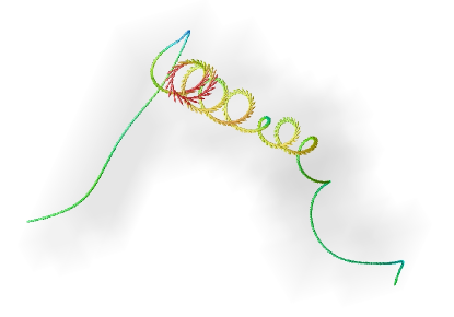
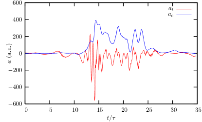
Figure 3: (Left panel) Trajectories with an intense value of the acceleration have been selected: as it can be seen, this corresponds to select tracers trapped into vortex filaments. Arrows and colors encode the velocity (magnitude and direction) of the particle. Rendering is realized with OpenDX. The movie (see multimedia enhancement) shows the flow as seen by riding this particle, before and during the trapping event. (Right panel) We show, in natural units, the behavior of one component of the centripetal and of the longitudinal acceleration (for details see the text). Notice the strong sign persistence of the centripetal acceleration with respect to the longitudinal one.

II Acceleration tails and spiraling motion

This and previous work cornell ; pinton ; biferale04 has collected evidence which highlights the relevance to Lagrangian turbulence of strong spiraling motions corresponding to trapping events, i.e. passive particles trapped in small scale vortex filaments. So we identify the strong bottleneck effect visible in Figure 1 and also the presence of extremely rare fluctuations in the pdf of the acceleration (see Figure 2). To illustrate better these strong events, we plot one of them in Figure 3. As is evident, the particle while moving slowly and smoothly, at some point gets trapped in a vortex filament and starts a spiraling motion characterized by huge values of the acceleration and by a “quasi-monochromatic” signal on all the velocity field components. Here, we suggest a way to characterize such events. This is of course a difficult task because not all the “trapping events” are so clearly detectable as that shown in Figure 3.

Indeed the motion of a particle in a turbulent field will be characterized by different accelerations and decelerations, not necessarily associated with spiraling motion (on average the mean value of the acceleration will be zero). In a spiraling motion the velocity ${\bm{v}}$ and acceleration ${\bm{a}}$ are orthogonal. Furthermore in a circular uniform motion the angular velocity, $\omega$, can be related to the centripetal acceleration $a_{c}=\omega^{2}r$ and to the linear velocity $v=\omega r$. We expect that in trapping events such as the one depicted in Fig. (3) the centripetal acceleration is intense and much more persistent than the longitudinal acceleration (i.e. the acceleration in the direction of the motion). To make this statement quantitative, we have studied the average of the centripetal, ${\bm{a}}_{c}={\bm{a}\times\hat{\bm{v}}}={\bm{a}\times{{\bm{v}}\over{|{\bm{v}}|}}}$, and longitudinal acceleration, ${\bm{a}}_{l}=({\bm{a}\cdot\hat{\bm{v}}}){\hat{\bm{v}}}$, over a time window which can vary up to $9\tau_{\eta}$, $\Delta=\{0.1,3,9\}\tau_{\eta}$:

$${\bm{a}}^{\Delta}_{c}(t)\equiv\left\langle{\bm{a}}_{c}\right\rangle_{\Delta}={1\over\Delta}\int_{t}^{t+\Delta}dt^{\prime}{\bm{a}}_{c}(t^{\prime});$$ (8)

$${\bm{a}}^{\Delta}_{l}(t)\equiv\left\langle{\bm{a}}_{l}\right\rangle_{\Delta}={1\over\Delta}\int_{t}^{t+\Delta}dt^{\prime}{\bm{a}}_{l}(t^{\prime}).$$ (9)

We expect that the pdfs of the averaged centripetal and longitudinal acceleration will behave very differently with increasing the window size, $\Delta$. In particular, the strong persistence of the centripetal acceleration up to $10\tau_{\eta}$ suggests that the centripetal pdf ${\cal P}({\bm{a}}^{\Delta}_{c})$ should remain almost unchanged when varying $\Delta$, while the longitudinal one ${\cal P}({\bm{a}}^{\Delta}_{l})$ should become less and less intermittent. This is what we show in Fig. (4).

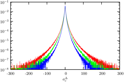
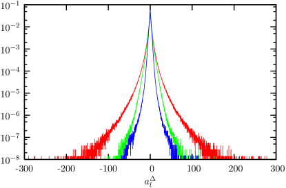
Figure 4: Pdf of the averaged centripetal $a_{c}$ (left panel), and longitudinal $a_{l}$ (right panel) acceleration components. The acceleration is averaged over a time window of size $\Delta=\{0.1,3,9\}\tau_{\eta}$ (respectively corresponding to colors red, green and blue).

In order to investigate further the role of trapping in vortices, we can define a typical radius of gyration $r_{c}$ and its typical eddy turnover time $\tau_{c}$, as:

$$r_{c}={|{\bm{v}}|^{2}\over{\left|{\bm{a}}\times{\hat{\bm{v}}}\right|}}\;\;\;\;\;\;\;\mbox{and}\;\;\;\;\;\;\;\tau_{c}={{\left|{\bm{v}}\right|}\over{\left|{\bm{a}}\times{\hat{\bm{v}}}\right|}}$$ (10)

Notice that using ${\bm{a}}\times{\hat{\bm{v}}}$ corresponds to selecting the centripetal values of the acceleration and hence augmenting the signal/noise ratio of spiraling motions with respect to the background of turbulent motions. The previous expressions applied to a typical vortex filament give $r_{c}\sim\eta$ and $\tau_{c}\sim\tau_{\eta}$. Similarly one may define a typical time based on the “longitudinal acceleration”: $\tau_{l}={{\left|{\bm{v}}\right|}/{\left|({\bm{a}}\cdot{\hat{\bm{v}}})\hat{\bm{v}}\right|}}$. Incoherent fluctuations with typical times of the order of $\tau_{\eta}$ should be averaged out once we measure the mean centripetal and longitudinal accelerations averaged over a window with $\Delta>\tau$ in expression (10). On the other hand, the signal coming from coherent vortex should not be affected by the averaging procedure and keeps its value: as a consequence, we should see events with $\tau_{c}\sim\tau_{\eta}$ even upon averaging. Going through Figure 5 we can observe, with increasing window size, the different behaviors of the pdfs of the centripetal and longitudinal characteristic times, $\tau_{c}$ and $\tau_{l}$ respectively. It is interesting to notice that the left tail of the centripetal pdf is quite robust, showing the presence of characteristic times of the order of $\tau_{c}\sim\tau_{\eta}$ even after averaging over a window with $\Delta=9\tau_{\eta}$. On the other hand the longitudinal characteristic times of order $\tau_{l}\sim\tau_{\eta}$ soon disappear as long as $\Delta\geq\tau_{\eta}$. We interpret this as further evidence of the importance of trapping in vortex filaments.

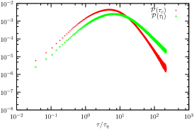
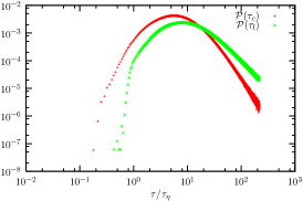
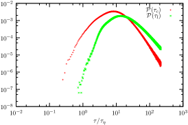
Figure 5: Pdf of the characteristic time estimated from the centripetal (in red) and longitudinal (in green) accelerations (in units of $\tau_{\eta}$) ${\cal P}(\tau_{c})$ and ${\cal P}(\tau_{l})$ respectively, for $\Delta=0.1\tau_{\eta}$ (left panel); $\Delta=3\tau_{\eta}$ (central panel); $\Delta=9\tau_{\eta}$ (right panel).

III Conclusions

We have presented results on the Lagrangian single-particle statistics from DNS of fully developed turbulence. In particular we have shown that (i) in the large time lag limit, $10\tau_{\eta}<\tau<T_{L}$, velocity structure functions are well reproduced by a standard adaptation of the Eulerian multifractal formalism to the Lagrangian framework; (ii) the acceleration statistics are also well captured by the multifractal prediction; (iii) for time lags of the order of the Kolmogorov time scale, $\tau_{\eta}$, up to time lags $10\tau_{\eta}$, the trapping by persistent vortex filaments may strongly affect the particle statistics. The last statement is supported both by the scaling of the Lagrangian statistics and by a new analysis based on the centripetal and longitudinal acceleration statistics.

References

References

- (1) Kraichnan RH 1965 Phys. Fluids 8 575.
- (2) Pope SB 2000 Turbulent Flows (Cambridge University Press, Cambridge).
- (3) La Porta A, Voth GA, Crawford AM, Alexander J and Bodenshatz E 2001 Nature 409 1017. Voth GA et al 2002 J. Fluid Mech. 469 121. Mordant N et al. 2003 Physica D 193 245.
- (4) Mordant N et al. 2003 J. Stat. Phys. 113 701. Mordant N et al. 2002 Phys. Rev. Lett. 89 254502. Mordant N et al. 2001 Phys. Rev. Lett. 87 214501.
- (5) Ott S and Mann J 2000 J. Fluid Mech. 422 207.
- (6) Chevillard L, Roux SG, Leveque E et al. 2003 Phys. Rev. Lett. 91 214502.
- (7) Yeung PK 2002 Ann. Rev. Fluid Mech. 34 115. Yeung PK 2001 J. Fluid Mech. 427 241. Vedula P and Yeung PK 1999 Phys. Fluids 11 1208.
- (8) Boffetta G. and Sokolov IM 2002 Phys. Rev. Lett. 88 094501.
- (9) Ishihara T and Kaneda Y 2002 Phys. Fluids 14 L69.
- (10) Beck C 2003 Europhys. Lett. 64 151. Beck C 2001 Phys. Lett. A 27 240.
- (11) Aringazin AK and Mazhitov MI 2003 Phys. Lett. A 313 284.
- (12) Arimitsu T and Arimitsu N 2003 Physica D 193 218.
- (13) Gotoh T and Kraichnan RH 2004 Physica D 193 231.
- (14) Biferale L, Boffetta G, Celani A, Lanotte A and Toschi F 2004 Particle trapping in fully developed turbulence http://arxiv.org/abs/nlin.CD/0402032.
- (15) Biferale L, Boffetta G, Celani A, Devenish BJ, Lanotte A, and Toschi F 2004 Phys. Rev. Lett. 93 064502.
- (16) Frisch U 1995 Turbulence: the legacy of A.N. Kolmogorov (Cambridge University Press, Cambridge).
- (17) Borgas MS 1993 Phil. Trans. R. Soc. Lond. A 342 379.
- (18) Boffetta G et al. 2002 Phys. Rev. E 66 066307.
- (19) Benzi R, Ciliberto S, Tripiccione R, Baudet C, Massaioli F and Succi S 1993 Phys. Rev. E 48 R29
- (20) She ZS and Lévêque E 1994 Phys. Rev. Lett. 72 336.