Characterization of chaotic dynamics in the vocalization of Cervus Elaphus Corsicanus

Angelo Facchini a.facchini@unisi.it Department of Chemical and Biosystems Sciences, University of Siena
Via della Diana 2/A 53100 Siena, Italy. Simone Bastianoni bastianoni@unisi.it Department of Chemical and Biosystems Sciences, University of Siena
Via della Diana 2/A 53100 Siena, Italy. Nadia Marchettini marchettini@unisi.it Department of Chemical and Biosystems Sciences, University of Siena
Via della Diana 2/A 53100 Siena, Italy. Mauro Rustici Corresponding Author rustici@uniss.it Department of Chemistry, University of Sassari, Via Vienna 2-I 07100 Sassari, Italy.

Abstract

Chaos, oscillations, instabilities, intermittency represent only some nonlinear examples apparent in natural world. These phenomena appear in any field of study, and advances in complex and nonlinear dynamic techniques bring about opportunities to better understand animal signals.

In this work we suggest an analysis method based on the characterization of the vocal fold dynamics by means of the nonlinear time series analysis, and by the computations of the parameters typical of chaotic oscillations: Attractor reconstruction, Spectrum of Lyapunov Exponents and Maximum Lyapunov Exponent was used to reconstruct the dynamic of the vocal folds. Identifying a sort of of vocal fingerprint can be useful in biodiversity monitoring and understanding the health status of a given animal.

This method was applied to the vocalization of the Cervus Elaphus Corsicanus, the Sardinian Red Deer.

pacs:

05.45.T, 43.80.ka [WA], 43.25.Rq [MFH], 43.72.Ar [DDO]

I Introduction

The physical and physiological mechanism of sound production are important to understanding mammal vocalization which ranges from periodic vocal fold vibrations to completely aperiodic vibration and atonal noise. Between these two extremes, a large amount of phenomena have been observed and reported m2 ; m4 : biphonation, cycles, subharmonic and chaotic behavior. These behaviors can be predicted by theoretical models. For example, the two mass model (the most accepted for mammal apparatus of phonation) can exhibit irregular oscillations 2masse ; jasa110-7 . The apparatus of phonation can be investigated through the characterization of the animal vocalization, where vocal nonlinearity can be used. According to Tokudatoku the nonlinear analysis of human speech signal has been carried out extensively, while nonlinear characteristics for animal voice signals have not yet been investigated.

Using the methods of nonlinear time series analysis we wished to understand the mechanics of the vocal folds starting from the vocalization time series. The characterization of the vocal signal as a chaotic time series can give important information on the health status of the animal, since the oscillation modes are related to the status of the throat tissues and to the strength of the animal. Furthermore tissues shapes of vocal apparatus are different among the animals and the characterization of several chaotic signals can be used in the monitoring of biodiversity.

The last remaining populations of a sub-specie of the red deer: the Sardinian deer (Cervus Elaphus Corsicanus) are found in the well preserved evergreen forest of Monte Arcosu in Sardinia (a protected area owned by WWF Italy). The Cervus Elaphus is the largest and most phylogenetically advanced species of Cervus. Head and body length is 1.65-2.65m, tail length is 0.11-0.27m, height at the shoulder is 0.75-0.15m, and weight is 75-340 kg. The largest and strongest male generally has the largest harem. In order to maintain this position of superiority he must constantly keep the distance with rival males by bellowing out, and chasing off potential rivals who come near his females. After vocalizing, the largest remaining males size each other up, and if antler and body size are comparable, they battle for the females. Their antlers lock and each male attempts to forcefully push the other away. The strongest and most powerful male wins and secures a harem (group) of females for mating. In this work an extensive characterization of the vocalization of Cervus Elaphus Corsicanus is presented by means of Lyapounov exponents of the chaotic oscillation evidence of registered sounds.

II Material

A number of different signals corresponding to different sound emissions were considered. Only clear and low noise sound emissions have been analyzed, in order to focus exclusively on meaningful vocalizations, and to avoid spurious effect. The vocalizations were recorded from adult males in their natural environment and digitized with a sampling frequency of 22050 Hz. Fig.1(b) shows a small portion of the analyzed signal and in Fig.1(d), the spectrogram (512 points FFT) of the signal is shown.

Discrete Fourier Transform (Fig.1(c)) was used to perform a preliminary spectral analysis on vocalization units. The presence of regions with high density of unresolved frequencies is a necessary, even if not sufficient, condition for the occurrence of chaotic dynamical regimes ott93 . Non-linear dynamics analysis were, therefore, was limited to signal units characterized by broad-band features in the frequency domain. Results reported in the present work refer to a single signal 0.420s long. The time series examined consists of a 9455 points sampled at 22050Hz.

III Computational methods

The analysis of the time series was performed using the software package TISEAN¹¹1The TISEAN software package is publicy available at http://www.mpipks-dresden.mpg.de/ $\sim$ tisean/TISEAN $\_2.1$ /index.html. (TIme SEries ANalysis) Kantz97 , valued as the most well known and robust algorithm set for nonlinear time series analysis. Typical steps are attractor reconstruction from time series and the characterization of the chaotic dynamic by means of Lyapunov exponents and maximum Lyapunov exponent (MLE).

III.1 Attractor reconstruction

The attractor of underlying dynamics has been reconstructed in phase space by applying the time delay vector method ott93 ; aba96 .

Starting from a time series $s(t)=[s_{1},\dots,s_{N}]$ the system dynamic can be reconstructed using the delay theorem by Takens and Mañe. The reconstructed trajectory $\mathbf{X}$ can be expressed as a matrix where each row is a phase space vector:

\mathbf{X}=[X_{1},X_{2},\dots,X_{M}]^{T}

(1)

where $X_{i}=[s_{i},s_{i+T},\dots,s_{i-(D_{E}-1)T}]$ and $M=N-(D_{E}-1)T$ .

The matrix is characterized by two key parameters: The Embedding Dimension $D_{E}$ and the Delay Time $T$ . The embedding dimension is the minimum dimension at which the reconstructed attractor can be considered completely unfolded and there is no overlapping in the reconstructed trajectories. If the chosen dimension is lower than $D_{E}$ the attractor is not completely unfolded and the underlying dynamics cannot be investigated. Higher dimension was not used due to the increase in computational effort.

The algorithm used for the computation of $D_{E}$ is the method of False Nearest Neighborsaba93 . A false neighbor is a point of trajectory intersection in a poorly reconstructed attractor. As the dimension increases, the attractor is unfolded with greater fidelity, and the number of false neighbors decreases to zero. The first dimension with no overlapping points is $D_{E}$ .

The delay time $T$ represents a measure of correlation existing between two consecutive components of $D_{E}$ -dimensional vectors used in the trajectory reconstruction. Following a commonly applied methodology, the time delay $T$ is chosen in correspondence to the first minimum of the average mutual information function fra86 .

III.2 Lyapunov exponents

Chaotic systems display a sensitive dependence on initial conditions. Such a property deeply affects the time evolution of trajectories starting from infinitesimally close initial conditions, and Lyapunov exponents are a measure of this dependence. These characteristic exponents give a coordinate independent measure of the local stability properties of a trajectory. If the trajectory evolves in a $N$ -dimensional state space there are $N$ exponents arranged in decreasing order, referred to as the Spectrum of Lyapunov Exponents (SLE):

\lambda_{1}\geq\lambda_{2}\geq\dots\geq\lambda_{n}

(2)

Conceptually these exponents are a generalizations of eigenvalues used to characterize different types of equilibrium points.

A trajectory is chaotic if there is at least one positive exponent, the value of this exponent, said the Maximum Lyapunov Exponent (MLE) gives a measure of the divergence rate of infinitesimally close trajectories and of the unpredictability of the system and gives a good characterization of the underlying dynamics.

Starting from the reconstructed attractor $\mathbf{X}$ , it is possible to compute with the method of Sano and SawadaGreene87 ; Sano85 the SLE consisting of exactly $n=D_{E}$ exponents. This method is a qualitative one, and in presence of a positive exponents, $\lambda_{1}$ , a more accurate method is necessary for the computation.

The method of Rosenstein-Kantzrose93 ; kantz94 is used to compute the MLE from the time series. This method measures in the reconstructed attractor the average divergence of two close trajectories in the time $d_{j}(i)$ . This can be expressed as:

d_{j}(i)=C_{j}e^{\lambda_{1}(i\Delta t)}

(3)

where $C_{j}$ is the initial separation. By taking the logarithm of both sides we obtain:

\ln d_{j}(i)=\ln C_{j}+\lambda_{1}(i\Delta t)

(4)

This is a set of approximately parallel lines (for $j=1,2,\dots,M$ ) each with a slope roughly proportional to $\lambda_{1}$ . The MLE is easily calculated using a least-squares fit to the average line defined by

y(i)=\frac{1}{\Delta t}\langle\ln d_{j}(i)\rangle

(5)

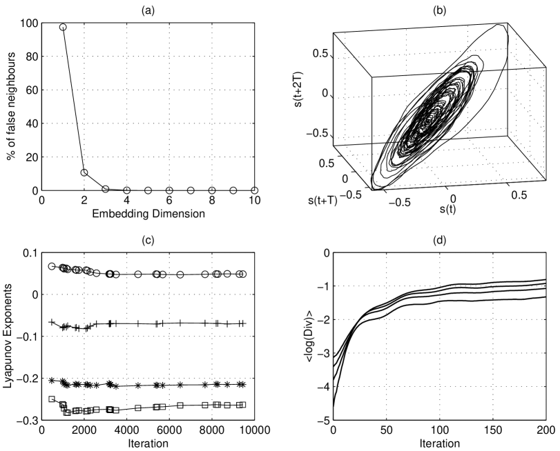
where $\langle\cdot\rangle$ denotes the average over all values of $j$ . Figure 2(d) shows a typical plot of $\langle\ln d_{j}(i)\rangle$ : after a short transition there is a linear region that is used to extract the MLE.

IV Results and Discussion

The signal considered was characterized by highly complex patterns in which different transients with both periodic and apparently aperiodic features were identified. The apparently random behavior of the numerical series, easily detectable with a simple visual inspection of the sound pattern, was confirmed by the power spectrum and spectrogram. Three different regions were put into evidence: at low frequencies, between 0 and 70 Hz, a first distribution of unresolved peaks is present, a sharp peak is also present at 450 Hz, while a broad band of frequencies, ranging between 850 and 1500 Hz, is easily detectable.

The chaotic characterization was performed calculating the embedding dimension $D_{E}$ by the false nearest method and in Fig.2(a) the result of the computation is shown. The figure reports the fraction of false neighbors with respect to the embedding dimension and a value of $D_{E}=4$ was found. The delay Time was considered as the first minimum of the mutual information function, and the value $T=8$ was found.

Starting from the time series the attractor was reconstructed using the delay method, and in Fig.2(b) a three dimensional projection of the attractor is shown. The structure of the attractors, related to the chaotic oscillation of the vocal folds, demonstrated that the irregular behavior observed in the time series was not due to noise.

In order to completely characterize the chaotic nature of the vocalization, the Spectrum of Lyapunov Exponents and the Maximum Lyapunov Exponent $\lambda_{1}$ were evaluated. In Fig.2(c) values of the four exponents are reported and the presence of a positive exponent was detected. The accurate value of the MLE was computed by the Rosenstein-Kantz method and a value of $\lambda_{1}=0.48$ was found by a linear regression of the curves in the region between 0 and 20 iterations.

The Kaplan-Yorke fractal dimension $D_{L}$ of the attractor kap79 , equal to $D_{L}=2.58$ , confirms the high dimensional fractal qualities of the strange attractor.

V Concluding remarks

The analysis method proposed in this letter was applied to the vocalization of an adult male of Cervus elaphus corsicanus and put in evidence the chaotic behavior of the irregolar oscillations in the signal considered. A full characterization by means of attractor reconstruction,Spectrum of Lyapunov Exponents, and Maximum Lyapunov Exponent was performed. A positive value of MLE was found. Future work aimed at identifying different individuals through the discussed parameters, will consist in the analysis of other vocalizations looking for a vocal fingerprint that may be useful in biodiversity monitoring.

Acknowledgements.

The authors are thankful to Dr. Carlo Murgia (Director of Oasi di monte Arcosu Sardegna) for providing the vocalizations.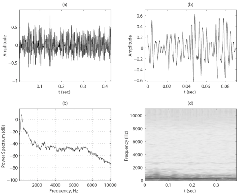

Refer to caption — Figure 1: (a) The analyzed signal. (b) A portion of the signal showing the irregular nature of the vocalization. (c) The power spectrum shows the typical Spectral contents of an irregular signal: a broadband and a continuous one. (d) The spectrogram of the signal showing a fundamental frequency of 70Hz and other frequencies until 2000Hz

Table 1: Results of the analysis performed on the vocalization signal. A positive Lyapunov exponent and the value of Kaplan-Yorke dimension indicates the chaotic nature of the signal.

Parameter	Value
Delay Time $\mathbf{T}$	8
Embedding Dimension $\mathbf{D_{E}}$	4
Maximum Lyapunov Exponent $\mathbf{\lambda_{1}}$	0.48
Kaplan-Yorke Dimension $\mathbf{D_{L}}$	2.58

References

(1) I.Wilden, H.Herzel, G.Peters, and G.Tembrock, “Subharmonics, biphonation and deterministic chaos in mammal vocalization,” Bioacoustics,171–196 (1998).
(2) I. Steinecke and H. Herzel, “Bifurcations in an asymmetric vocal fold model,” J. Acoustical Soc. of America 97(3), 1874–1884 (1995).
(3) H.Herzel, D.Berry, I.Titze, and I.Steincke, “Nonlinear dynamics of the voice: Signal analysis and biomechanical modeling,” CHAOS 5(1), 30–34 (1995).
(4) J.J.Jiang, Y.Zhang, and J.Stern, “Modeling of chaotic vibrations in symmetric vocal folds,” J. Acoust. Soc. Am. 110(4), 2120–2128 (2001).
(5) I.Tokuda, T.Reide, J.Neubauer, M.J.Owren, and H.Herzel, “Nonlinear analysis of irregular animal vocalizations,” J. Acoust. Soc. Am 111(6), 2908–2919 (2002).
(6) E.Ott, Chaos in dynamical systems (Cambridge University Press, UK, 1993).
(7) H.Kantz and T.Schreiber, Nonlinear Time Series Analysis (Cambridge University Press, UK, 1997).
(8) H.D.I.Abarbanel, Analysis of observed chaotic data (Springer-Verlag, ADDRESS, 1996).
(9) H.D.I.Abarbanel and M.B.Kennel, “Local false nearest neighbours and dynamical dimensions from observed chaotic data,” Phys. Rev. E 47, 3057 (1993).
(10) A.M.Fraser and H.L.Swinney, “Independent coordinates for strange attractors from mutual information,” Phys. Rev. A 33, 1134 (1986).
(11) J.M.Greene and J.S.Kim, “The calculation of lyapunov spectra,” Physica D 24, 213–225 (1987).
(12) M.Sano and Y.Sawada, “Measurement of the lyapunov spectrum from a chaotic time series,” Phys. Rev. Lett. 55, 1082 (1985).
(13) M.T.Rosenstein, J.J.Collins, and C. Luca, “A practical method for calculating largest lyapunov exponent from small data set,” Physica D 65, 117 (1993).
(14) H. Kantz, “A robust method to estimate the maximal lyapunov exponent of a time series,” Phys. Lett. A 185, 77 (1994).
(15) J. Kaplan and J. A. Yorke, Chaotic behaviour of multidimensional difference equation, Vol. 730 of lecture notes in mathematics (Springer Verlag, Berlin, 1979).