Changing shapes: adiabatic dynamics of composite solitary waves

Abstract

We discuss the solitary wave solutions of a particular two-component scalar field model in two-dimensional Minkowski space. These solitary waves involve one, two or four lumps of energy. The adiabatic motion of these composite non-linear non-dispersive waves points to variations in shape.

1 Introduction

A solitary wave travels “without changing its shape, size, or, speed”, [2]. In this paper we shall deal with solitary waves in relativistic scalar field theory in a two-dimensional space-time. Besides the prototypes, the kink of the non-linear Klein-Gordon equation and the sine-Gordon soliton found in models where the scalar field has only one component, solitary waves have also been discovered in systems with two-component scalar fields, [3]-[4].

In a deformed $O(2)$ Linear Sigma model, the celebrated Montonen-Sarker-Trullinger-Bishop (MSTB) model, see [5], [6], there exist solitary waves with two non-null field components. The model was first proposed by Montonen [5], and Sarker, Trullinger and Bishop [6] in the search for non-topological solitons. Nevertheless, in both papers the existence of two kinds of solitary waves, respectively with one and two non-null components, was noticed. Slightly later, Rajaraman and Weinberg [3] proposed the trial-orbit method to study the two-dimensional mechanical problem equivalent to the search for static solutions. By these means, they found that the TK1 -one-component topological- kink is given by a straight line trajectory in field space, whereas the TK2 -two-component topological- kinks come from semi-elliptic trajectories; they also enlarged the list by discovering NTK2 -two-component non-topological- kinks bound to elliptic orbits. Through numerical analysis, [7], [8], Subbaswamy and Trullinger, looking for more exotic orbits, observed the existence of a one-parametric family of NTK2, including that previously discovered in [3]. Moreover, they discovered an unexpected fact; the “kink energy sum rule”: NTK2 energy is the same as the addition of TK1 and TK2 energies. Magyari and Thomas, [9], realized that the reason for the sum rule lies in the integrability of the equivalent mechanical problem. Ito went further to show that the mechanical problem giving the solitary waves as separatrix trajectories in the MSTB model is not only integrable but also Hamilton-Jacobi separable, [10], and, moreover, distinguished between stable and unstable solitary waves, see [11], by applying the Morse index theorem. The full Morse Theory for the MSTB model was developed by one of us in [12].

Only TK2 kinks are stable and genuine solitary waves in the sense that they travel without distortion in shape, size, and, velocity. In a model proposed by Bazeia-Nascimento-Ribeiro and Toledo -henceforth the BNRT model, [13], [14] - things are different. In this case, both the TK1 and the TK2 kinks -discovered in the papers quoted above- are stable and degenerate in energy. In fact, they are distinguished members of a one-parametric family of kinks found in [15], all of them degenerate in energy, but composite in a certain sense. Apart from the center of the kink, there is a second integration constant; for large values of the second integration constant $b$ solitary waves seem to be composed of two lumps of energy, whereas for $b$ small they only show one lump. In References [16] and [17] we first unveiled the whole manifold of solitary waves of this model and then showed that in this system solitary waves can travel without dispersion, although changing the relative position of the two lumps.

The distribution of the lumps is, however, completely symmetric with respect to the center of mass. In this paper, we shall study a similar system to the MSTB and BNRT models in this framework. The model can be understood as the dimensional reduction of the planar Chern-Simons-Higgs model, [20], to a line and zero gauge field. The whole manifold of composite solitary waves was described in Reference [18]. We shall again derive the solitary wave solutions of the model called A in the Reference cited, now using the Bogomol’ny method, see [19]. This strategy is better suited for describing the wave properties than the solution of the Hamilton-Jacobi equation. Later, Manton’s adiabatic principle, designed to elucidate the slow-motion dynamics of topological defects, [23], will be applied to our solitary waves.

The organization of this paper is as follows: In Section §.2 we introduce the model and describe the spontaneous symmetry-breaking scenario. We also identify two systems of first-order differential equations that are satisfied by solitary waves using the Bogomol’nyi procedure. In Section §.3, the solitary wave solutions of the first-order equations will be obtained. We shall show that there exist two basic kink-shaped solitary waves and that the rest of the kinks are configurations of two or four basic kinks. The problem of the stability of these waves will be also addressed in this Section; the double solitary waves are stable whereas quadruple kinks are unstable. In Section §.4, we apply Manton’s principle to study the adiabatic dynamics of solitary waves as geodesic motion in their moduli space. There is no problem with double solitary waves but we also analyze the motion of quadruple lumps by pushing them in the direction of instability in configuration space. Finally, we explore how the system react to a small perturbation of the potential term, preserving the basic kinks; the induced forces give rise to a remarkable bound state of kinks, similar to the breather mode of sine-Gordon theory.

2 The model: quintic non-linear Klein-Gordon equation

We shall focus on a (1+1)-dimensional relativistic scalar field theory model, whose dynamics is governed by the action:

$$S=\int dy^{2}\left\{\frac{1}{2}\partial_{\mu}\chi^{*}\partial^{\mu}\chi-U(\chi,\chi^{*})\right\}$$ (1)

and $\chi(y_{\mu})=\chi_{1}(y_{\mu})+i\chi_{2}(y_{\mu}):{\mathbb{R}}^{1,1}\longrightarrow{\mathbb{C}}$ is a complex scalar field. We choose $g_{00}=-g_{11}=1$ and $g_{12}=g_{21}=0$ as the metric tensor components in Minkowski space ${\mathbb{R}}^{1,1}$, whereas

$$U[\chi,\chi^{*}]=\textstyle\frac{\lambda^{4}}{4m^{2}}\chi^{*}\chi\left(\chi^{*}\chi-\frac{m^{2}}{\lambda^{2}}\right)^{2}+\frac{\beta^{2}}{2}\chi_{2}^{2}\left[\chi^{*}\chi-\frac{m^{2}}{\lambda^{2}}\left(1-\frac{\beta^{2}}{2\lambda^{2}}\right)\right]$$

sets the non-linear interactions in (1). $\lambda$, $m$ and $\beta$ are coupling constants of inverse length dimension. Introducing non-dimensional variables $\chi=\frac{m}{\lambda}\phi$, $y_{\mu}=\frac{\sqrt{2}}{m}x_{\mu}$ and $\frac{\beta^{2}}{\lambda^{2}}=\sigma^{2}$, the action functional reads:

$$S=\frac{m^{2}}{\lambda^{2}}\int d^{2}x\left[\frac{1}{2}\partial_{\mu}\phi^{*}\partial^{\mu}\phi-V(\phi,\phi^{*})\right]$$

$$V(\phi,\phi^{*})=\frac{1}{2}\,\phi^{*}\phi\,(\phi^{*}\phi-1)^{2}+\sigma^{2}\phi_{2}^{2}\left(\phi^{*}\phi-1+\frac{\sigma^{2}}{2}\right)\qquad.$$ (2)

$-V(\phi,\phi^{*})$ -plotted in Figure 1a- is a semi-definite negative polynomial expression of degree six which depends on the unique classically relevant non-dimensional coupling constant $\sigma$.

Although the potential that we have chosen seems to be very awkward it is physically interesting for two reasons. First, $V(\phi_{1},\phi_{2})$ is a deformation of $V_{{\rm CSH}}(\phi)=\frac{1}{2}\,\phi^{*}\phi\,(\phi^{*}\phi-1)^{2}$ that appears in the celebrated Chern-Simons-Higgs model, see [20] and References quoted therein. The CSH model is a (2+1)-dimensional gauge field theory for a complex scalar (Higgs) field where the kinetic term for the gauge field in the Lagrangian is the first Chern-Simons secondary class, whereas the Higgs self-interaction is ruled by $V_{\rm CSH}$. A phenomenological theory for the fractionary quantum Hall effect has been established on the basis of a non-relativistic version of the CSH model in [21]. Dimensional reduction to (1+1)-dimensions at zero gauge field leads to a class of systems including our model because there are no Goldstone bosons on the line [22]; the infrared asymptotic behavior of the quantum theory would require the modification of $V_{CSH}$ in such a way that the zeroes become a discrete set and massless particles are forbidden. The deformation of our choice comply with this requirement and, moreover, ensures integrability of the dynamical system to be solved in the search for kinks. Second, we shall show in Section §3 that the Hamilton characteristic function, the “superpotential” $W^{I}(\phi)$ (16), is precisely the potential of the MSTB model. This fact links both systems in a hierarchal way.

The second term in (2) breaks the $U(1)$ symmetry of this model. The ${\mathbb{G}}={\mathbb{Z}}_{2}\times{\mathbb{Z}}_{2}$ group, generated by the reflections $\phi_{1}\rightarrow-\phi_{1}$ and $\phi_{2}\rightarrow-\phi_{2}$ in the internal space ${\mathbb{C}}$, leaves, however, our system invariant.

         

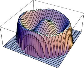
Figure 1: a) Potential term $-V(\phi,\phi^{*})$. b) Set of zeroes ${\cal M}$ of $-V(\phi,\phi^{*})$.

The field equations form the following system of coupled second-order PDE:

$$\frac{\partial^{2}\phi_{1}}{\partial t^{2}}-\frac{\partial^{2}\phi_{1}}{\partial x^{2}} = -\phi_{1}[1+3\phi_{1}^{4}+3\phi_{2}^{4}+\phi_{1}^{2}(6\phi_{2}^{2}-4)+2(\sigma^{2}-2)\phi_{2}^{2}]$$ (3)

$$\frac{\partial^{2}\phi_{2}}{\partial t^{2}}-\frac{\partial^{2}\phi_{2}}{\partial x^{2}} = -\phi_{2}[3\phi_{1}^{4}+2\phi_{1}^{2}(3\phi_{2}^{2}+\sigma^{2}-2)+(\phi_{2}^{2}+\sigma^{2}-1)(3\phi_{2}^{2}+\sigma^{2}-1)]\qquad.$$ (4)

The PDE system (3), (4) is akin to the non-linear Klein-Gordon equation with quintic -besides cubic- non-linear terms. Initial, $\phi(t_{0},x)$, $\frac{\partial\phi}{\partial t}(t_{0},x)$, and/or boundary conditions, $\phi(t,\pm x_{0})$, $\frac{\partial\phi}{\partial x}(t,\pm x_{0})$, must be chosen in order to search for physically relevant solutions. We focus our attention on those solutions that can be interpreted as lumps or extended particles: that is, solitary waves or kinks. Recall the definition of a solitary wave, see e.g. [4]: “A solitary wave is a localized non-singular solution of any non-linear field equation whose energy density, as well as being localized, has space-time dependence of the form: $\varepsilon(t,x)=\varepsilon(x-\mbox{v}t)$, where v is some velocity vector”.

2.1 Structure of the configuration space

The set of zeroes of $V(\phi_{1},\phi_{2})$ -maxima of $-V(\phi_{1},\phi_{2})$- is:

$${\cal M}=\{\bar{\phi}^{A^{\pm}}=\pm 1;\,\bar{\phi}^{B^{\pm}}=\pm i\bar{\sigma};\,\bar{\phi}^{O}=0\}\qquad,\qquad\bar{\sigma}=\sqrt{1-\sigma^{2}}$$

see Figure 1b. These constant configurations are the static homogeneous solutions of the PDE system (3), (4) because they are critical points of $V(\phi_{1},\phi_{2})$: $\frac{\partial V}{\partial\phi_{1}}=0=\frac{\partial V}{\partial\phi_{2}}$. Note that the reflection $\phi_{1}\rightarrow-\phi_{1}$ sends $\bar{\phi}^{A^{+}}$ to $\bar{\phi}^{A^{-}}$ and vice-versa; they belong to the same ${\mathbb{G}}$-equivalence class: $\bar{\phi}^{A}=\{\bar{\phi}^{A^{+}},\bar{\phi}^{A^{-}}\}$. There are another two ${\mathbb{G}}$-orbits between the constant solutions: $\bar{\phi}^{B}=\{\bar{\phi}^{B^{+}},\bar{\phi}^{B^{-}}\}$ and $\bar{\phi}^{O}$. The moduli space of homogeneous solutions- i.e., the set of zeroes of $V$ modulo the symmetry group- consists of three points in ${\mathbb{C}}$: $\bar{\cal M}=\frac{{\cal M}}{{\mathbb{G}}}=\{\bar{\phi}^{A},\bar{\phi}^{B},\bar{\phi}^{O}\}$. The degeneracy of the homogeneous solutions -all of them have zero energy- causes spontaneous breaking of the discrete symmetry. The constant solution $\bar{\phi}^{A}$ breaks the symmetry under ${\mathbb{G}}={\mathbb{Z}}_{2}\times{\mathbb{Z}}_{2}$ transformations of the action functional (1) to the little group $H_{1}=\{e\}\times{\mathbb{Z}_{2}}$ generated by $\phi_{2}\rightarrow-\phi_{2}$. Simili modo, the remaining symmetry group at $\bar{\phi}^{B}$ is the $H_{2}={\mathbb{Z}_{2}}\times\{e\}$ little group generated by $\phi_{1}\rightarrow-\phi_{1}$, whereas the point $\bar{\phi}^{O}$ preserves the full symmetry ${\mathbb{G}}$.

The configuration space of the system ${\cal C}=\{\phi(t,x)\in{\rm Maps}({\mathbb{R}},{\mathbb{C}})\hskip 8.5359pt/\hskip 8.5359pt{\cal E}[\phi]<\infty\}$ is the set of maps from ${\mathbb{R}}$ to ${\mathbb{C}}$ for fixed time $t$ such that the energy functional

$${\cal E}[\phi]=\int dx\left\{\frac{1}{2}\,\left(\frac{\partial\phi_{1}}{\partial x}\right)^{2}+\frac{1}{2}\,\left(\frac{\partial\phi_{2}}{\partial x}\right)^{2}+V(\phi_{1},\phi_{2})\right\}$$ (5)

is finite. Thus, every configuration in ${\cal C}$ must comply with the asymptotic conditions:

$$\lim_{x\rightarrow\pm\infty}\phi(t,x)\in{\cal M}\hskip 56.9055pt\lim_{x\rightarrow\pm\infty}\frac{\partial\phi(t,x)}{\partial x}=0\qquad.$$ (6)

These asymptotic conditions play an important r$\hat{{\rm o}}$le from a topological point of view. The configuration space is the union of 25 topologically disconnected sectors:

$${\cal C}= \,\,\,\,{\cal C}^{AA}_{\pm\pm}\,\sqcup\,\,{\cal C}^{BB}_{\pm\pm}\,\sqcup\,\,{\cal C}^{OO}\,\sqcup\,\,{\cal C}^{AA}_{\pm\mp}\,\sqcup\,\,{\cal C}^{BB}_{\pm\mp}$$ (7)

$$\,\sqcup\,\,{\cal C}^{AB}_{\pm\pm}\,\sqcup\,\,{\cal C}^{BA}_{\pm\pm}\,\sqcup\,\,{\cal C}^{AB}_{\pm\mp}\,\sqcup\,\,{\cal C}^{BA}_{\pm\mp}$$

$$\,\sqcup\,\,{\cal C}^{AO}_{\pm}\,\sqcup\,\,{\cal C}^{OA}_{\pm}\,\sqcup\,\,{\cal C}^{BO}_{\pm}\,\sqcup\,\,{\cal C}^{OB}_{\pm}$$

The relation of this notation to the asymptotic conditions (6) is self-explanatory. Three examples:

1. Sector ${\cal C}^{OO}$. Boundary conditions:

   $$\lim_{x\rightarrow-\infty}\phi(t,x)=\bar{\phi}^{O}\hskip 56.9055pt,\hskip 56.9055pt\lim_{x\rightarrow\infty}\,\phi(t,x)=\bar{\phi}^{O}$$

2. Sector ${\cal C}^{AB}_{\pm\pm}$. Boundary conditions:

   $$\lim_{x\rightarrow-\infty}\phi(t,x)=\bar{\phi}^{A_{\pm}}\hskip 56.9055pt,\hskip 56.9055pt\lim_{x\rightarrow\infty}\,\phi(t,x)=\bar{\phi}^{B_{\pm}}$$

3. Sector ${\cal C}^{BA}_{\pm\mp}$. Boundary conditions:

   $$\lim_{x\rightarrow-\infty}\phi(t,x)=\bar{\phi}^{B_{\pm}}\hskip 56.9055pt,\hskip 56.9055pt\lim_{x\rightarrow\infty}\,\phi(t,x)=\bar{\phi}^{A_{\mp}}$$

Because temporal evolution is continuous (a homotopy transformation), the asymptotic conditions (6) do not change with $t$ and the 25 sectors (7) are completely disconnected. Physically this means that a solution in a sector cannot decay into solutions belonging to other different sectors; it would cost infinite energy.

The five homogeneous solutions of (3)-(4) that are zeroes of $V$ belong to the five sectors ${\cal C}^{AA}_{\pm\pm}$, ${\cal C}^{BB}_{\pm\pm}$ and ${\cal C}^{OO}$ respectively. Small fluctuations around one of them, $\psi(t,x)=\bar{\phi}+\delta\psi(t,x)$, $\bar{\phi}\in{\cal M}$, solve the linear PDE system:

$$\sum_{b=1}^{2}\left(\Box\delta_{ab}+M^{2}_{ab}(\bar{\phi})\right)\delta\psi_{b}(t,x)=0\qquad,\qquad M^{2}_{ab}(\bar{\phi})=\frac{\partial^{2}V}{\partial\phi_{a}\partial\phi_{b}}(\bar{\phi})$$ (8)

The solution of (8) via the separation of variables -$\delta\psi_{a}(t,x)={\rm exp}[i\omega t]f_{a}^{\omega}(x)$- leads to the spectral problem for the second order fluctuation -or Hessian- operator:

$${\cal H}(\bar{\phi})\left(\begin{array}[]{c}f_{1}^{\omega}(x)\\ f_{2}^{\omega}(x)\end{array}\right)=\left(\begin{array}[]{cc}-{d^{2}\over dx^{2}}+M^{2}_{11}(\bar{\phi})&M^{2}_{12}(\bar{\phi})\\ M^{2}_{21}(\bar{\phi})&-{d^{2}\over dx^{2}}+M^{2}_{22}(\bar{\phi})\end{array}\right)\left(\begin{array}[]{c}f_{1}^{\omega}(x)\\ f_{2}^{\omega}(x)\end{array}\right)=\omega^{2}\left(\begin{array}[]{c}f_{1}^{\omega}(x)\\ f_{2}^{\omega}(x)\end{array}\right)$$

${\cal H}(\bar{\phi})$ is a diagonal matrix differential operator for the three points of $\bar{\cal M}$ with a positive definite spectrum; every constant solution belonging to ${\cal M}$ is stable. Thus, there are three types of dispersive wave-packet solutions, living respectively in one of these sectors. The building blocks are plane waves with their dispersion laws respectively determined by:

$$\begin{array}[]{ccccc}{M^{2}(\bar{\phi}^{A})=\left(\begin{array}[]{cc}4&0\\ 0&\sigma^{4}\end{array}\right)}&&{M^{2}(\bar{\phi}^{B})=\left(\begin{array}[]{cc}\sigma^{4}&0\\ 0&4\bar{\sigma}^{4}\end{array}\right)}&&{M^{2}(\bar{\phi}^{O})=\left(\begin{array}[]{cc}1&0\\ 0&\bar{\sigma}^{4}\end{array}\right)}\end{array}\qquad.$$

The two branches for each type are:

$$\begin{array}[]{|cc|c|cc|}\hline\cr&&&&\\[-8.5359pt] \bar{\phi}^{A}&&\bar{\phi}^{B}&&\bar{\phi}^{O}\\ \hline\cr&&&&\\[-8.5359pt] \omega^{2}(k)=k^{2}+4&&\omega^{2}(k)=k^{2}+\sigma^{4}&&\omega^{2}(k)=k^{2}+1\\ \omega^{2}(q)=q^{2}+\sigma^{4}&&\omega^{2}(q)=q^{2}+4\sigma^{4}&&\omega^{2}(q)=q^{2}+\bar{\sigma}^{4}\\ \hline\cr\end{array}$$

2.2 Solitary waves from integrable dynamical systems

Any other static solution of (3)-(4) is a solitary wave that lives in one of the remaining twenty topological sectors of the configuration space. The field profiles can be either kink- or bell-shaped, and Lorentz invariance allows the use of the center of mass system. The energy density and field equations read:

$$\varepsilon(x)={1\over 2}\left(\frac{d\phi_{1}}{dx}\right)^{2}+{1\over 2}\left(\frac{d\phi_{2}}{dx}\right)^{2}+V(\phi_{1},\phi_{2})\hskip 28.45274pt;\hskip 28.45274pt{d^{2}\phi_{a}\over dx^{2}}={\partial V\over\partial\phi_{a}}\quad,\quad a=1,2\qquad.$$ (9)

The search for solitary waves is tantamount to the search for finite energy static solutions $\phi(x)$ of the PDE system (3)-(4), which, in turn, reduces to the ODE system (9). A Lorentz transformation sends the static solution $\phi(x)$ to $\phi(t,x)=\phi\left(\frac{x-{\rm v}t}{\sqrt{1-{\rm v}^{2}}}\right)$.

The ODE system (9) is nothing more than the equations of motion for a two-dimensional mechanical system: understand $(\phi_{1},\phi_{2})$ as the “particle” coordinates; $x$ as the “particle” time, and $U=-V$ as the “particle” potential energy. We shall use a mixture of Hamilton-Jacobi and Bogomol’nyi procedures to solve this system.

$$V(\phi_{1},\phi_{2})=\frac{1}{2}\left(\frac{\partial W}{\partial\phi^{1}}\right)^{2}+\frac{1}{2}\left(\frac{\partial W}{\partial\phi^{2}}\right)^{2}$$ (10)

is the “time”-independent Hamilton-Jacobi equation for the mechanical system and zero “particle” energy. Using the Hamilton characteristic function $W$, the solution of (10), we write the field theory potential energy for static configurations $\grave{a}$ $la$ Bogomol’nyi:

$${\cal E}[\phi_{1},\phi_{2}] = \int\!dx\,\frac{1}{2}\left[\left(\frac{d\phi^{1}}{dx}\right)^{2}+\left(\frac{d\phi^{2}}{dx}\right)^{2}+\left(\frac{\partial W}{\partial\phi^{1}}\right)^{2}+\left(\frac{\partial W}{\partial\phi^{2}}\right)^{2}\right]$$ (11)

$$= \frac{1}{2}\int_{-\infty}^{\infty}dx\left[\left(\frac{d\phi^{1}}{dx}-\frac{\partial W}{\partial\phi^{1}}\right)^{2}+\left(\frac{d\phi^{2}}{dx}-\frac{\partial W}{\partial\phi^{2}}\right)^{2}\right]+|\cal{T}|\qquad.$$

Here,

$${\cal T}=\int_{-\infty}^{\infty}dx\left(\frac{d\phi^{1}}{dx}\frac{\partial W}{\partial\phi^{1}}+\frac{d\phi^{2}}{dx}\frac{\partial W}{\partial\phi^{2}}\right)=\int\,\,dW$$ (12)

is a topological charge, depending only on the sector of the configuration space if $W$ is well-behaved enough to apply Stokes theorem:

$${\cal T}=W(\phi_{1}(\infty),\phi_{2}(\infty))-W(\phi_{1}(-\infty),\phi_{2}(-\infty))\qquad.$$

In this case, an absolute minimum of the field theory energy (11), in the corresponding topological sector, is reached by the solutions of the following system of first-order equations:

$$\frac{d\phi_{1}}{dx}=\frac{\partial W}{\partial\phi_{1}}\hskip 28.45274pt;\hskip 28.45274pt\frac{d\phi_{2}}{dx}=\frac{\partial W}{\partial\phi_{2}}\qquad;$$ (13)

(in (11) the squared terms are always positive and the other is a topological constant). It is easy to check that solutions of the first-order equations (13) also solve the second-order (Euler-Lagrange) equations (9) and consequently (3) and (4). The energy of these solutions depends only on the topological sector of the solitary wave, and it saturates the topological bound $\cal{E}[\phi_{\rm K}]=|{\cal T}|$. The quotient of the first by the second first-order equations gives the “orbits”:

$$\frac{\partial W}{\partial\phi_{2}}d\phi_{1}=\frac{\partial W}{\partial\phi_{1}}d\phi_{2}\qquad.$$ (14)

$$\left\{\frac{\partial W}{\partial\phi_{1}}(\phi_{1},\tilde{\phi_{2}}(\phi_{1}))\right\}^{-1}d\phi_{1}=dx\hskip 14.22636pt,\hskip 14.22636pt\left\{\frac{\partial W}{\partial\phi_{2}}(\tilde{\phi_{1}}(\phi_{2}),\phi_{2})\right\}^{-1}d\phi_{2}=dx\qquad,$$ (15)

where $\tilde{\phi}_{1}(\phi_{2})$ (respectively $\tilde{\phi}_{2}(\phi_{1})$) is a solution of (14), provide the “time”-schedules of the “particle”. In fact, this system of three equations would be also obtained in the Hamilton-Jacobi framework setting all the separation constants equal to zero.

3 The variety of solitary waves

Using elliptic coordinates,

$$u(x)={1\over 2}\left(\sqrt{(\phi_{1}(x)+\sigma)^{2}+\phi_{2}^{2}(x)}+\sqrt{(\phi_{1}(x)-\sigma)^{2}+\phi_{2}^{2}(x)}\right)\in(\sigma,+\infty)$$

$$v(x)={1\over 2}\left(\sqrt{(\phi_{1}(x)+\sigma)^{2}+\phi_{2}^{2}(x)}-\sqrt{(\phi_{1}(x)-\sigma)^{2}+\phi_{2}^{2}(x)}\right)\in(-\sigma,\sigma)\qquad,$$

one can show that the equation (10) is separable for our choice of $V(\phi_{1},\phi_{2})$. Thus, two independent solutions for $W$ as a function of $u,v$ are found. Back in Cartesian coordinates, these are:

$$W^{I}(\phi)=\frac{1}{4}\left[(\phi_{1}^{2}+\phi_{2}^{2}-1)^{2}+2\sigma^{2}\phi_{2}^{2}\right]\qquad,$$ (16)

$$W^{II}(\phi)=\frac{1}{4}\,\sqrt{(\phi_{1}+\sigma)^{2}+\phi_{2}^{2}}\,\sqrt{(\phi_{1}-\sigma)^{2}+\phi_{2}^{2}}\,(\phi_{1}^{2}+\phi_{2}^{2}+\sigma^{2}-2)\qquad.$$ (17)

$W^{I}$ is a polynomial function of $\phi_{1},\phi_{2}$ without singularities and everything proceeds smoothly. The partial derivatives of $W^{II}$, however, are undefined at the points $(\phi_{1}=\pm\sigma,\phi_{2}=0)$; it is uncertain how to interpret this second solution of the Hamilton-Jacobi equation. Note also that if a function $W(\phi)$ verifies formula (10) then $-W(\phi)$ also satisfies this condition. Replacing $W$ by $-W$ merely flips the sign of the topological charge.

The system of first-order differential equations (13) determined by the first solution $W^{I}$ is:

$$\left\{\begin{array}[]{l}\displaystyle\frac{d\phi_{1}}{dx}=\phi_{1}(\phi_{1}^{2}+\phi_{2}^{2}-1)\\[11.38092pt] \displaystyle\frac{d\phi_{2}}{dx}=\phi_{2}(\phi_{1}^{2}+\phi_{2}^{2}-1+\sigma^{2})\end{array}\right.\qquad,$$ (18)

whereas the flow of the gradient of the second solution $W^{II}$ is ruled by the first-order ODE system:

$$\left\{\begin{array}[]{l}\displaystyle\frac{d\phi_{1}}{dx}=\frac{\phi_{1}[\phi_{1}^{4}+\phi_{2}^{4}+\sigma^{2}+\phi_{1}^{2}(2\phi_{2}^{2}-1-\sigma^{2})+\phi_{2}^{2}(\sigma^{2}-1)]}{\sqrt{(\phi_{1}-\sigma)^{2}+\phi_{2}^{2}}\sqrt{(\phi_{1}+\sigma)^{2}+\phi_{2}^{2}}}\\[14.22636pt] \displaystyle\frac{d\phi_{2}}{dx}=\frac{\phi_{2}[\phi_{1}^{4}+\phi_{2}^{4}+\phi_{1}^{2}(2\phi_{2}^{2}-1)+\sigma^{2}(\sigma^{2}-1)+\phi_{2}^{2}(2\sigma^{2}-1)]}{\sqrt{(\phi_{1}-\sigma)^{2}+\phi_{2}^{2}}\sqrt{(\phi_{1}+\sigma)^{2}+\phi_{2}^{2}}}\end{array}\right.\qquad.$$ (19)

3.1 Solitary waves: basic types

In order to solve the ODE systems (18) and (19) we start by looking for restrictions on $\phi$ that make both systems coincide. The idea is akin to the Rajaraman trial-orbit method, see [4]: guess a trajectory that joins two points in $\bar{\cal M}$ and minimizes ${\cal E}$. It happens that there are two types of curves in ${\mathbb{C}}$ for which (18) and (19) become identical; they provide the basic solitary waves of the model.

1. K${}_{1}^{BO}$: We shall now try the condition $\bar{\phi}_{1}=0$ in systems (18) and/or (19). We find kink solutions joining the points $O$ and $B$ in the moduli space:

   $$\bar{\phi}(x;a)=(-1)^{\alpha}\,i\,\frac{\bar{\sigma}}{\sqrt{2}}\,\sqrt{1\,+(-1)^{\beta}\,{\rm tanh}\,[\bar{\sigma}^{2}(x-a)]}\hskip 28.45274pt\alpha,\beta=0,1$$ (20)

   Because the orbits stay on the straight line $\bar{v}=0$ in the elliptic plane joining $B$ with $O$, we shall refer to these four solutions -here we consider the parameter $a$ to be fixed- as K${}_{1}^{BO}$. A solitary wave connects the points $O$ and $B_{+}$ if $\alpha=\beta=0$ and the points $O$ and $B_{-}$ if $\alpha=1,\beta=0$ -living respectively in ${\cal C}^{OB}_{\pm}$-. For the cases $\alpha=0,\beta=1$ and $\alpha=\beta=1$, we find respectively the antikinks of the above mentioned solutions. One of these solutions has been depicted in Figure 2, in addition to its density energy and its orbit in the internal complex plane. In Figure 2c, we see why these solitary waves are interpreted as lumps of energy or extended particles. The energy of these solutions is:

   $${\cal E}[{\rm K_{1}^{BO}}]=|T|=\left|W^{I}[\bar{\phi}^{B}]-W^{I}[\bar{\phi}^{O}]\right|=\left|W^{II}[\bar{\phi}^{B}]-W^{II}[\bar{\phi}^{O}]\right|=\left(\frac{1}{2}-\frac{\sigma^{2}}{2}\right)^{2}\,\,.$$

              

   Figure 2: K${}_{1}^{BO}$ Kink: a) Orbit, b) Kink profiles and c) Energy density.

2. K${}_{1}^{AB}$: On the ellipse $\bar{\phi}_{1}^{2}+\frac{\bar{\phi}_{2}^{2}}{1-\sigma^{2}}=1$ -$\bar{u}=1$ in the elliptic plane - (see Figure 3a), equations (18) and (19) also coincide. The following eight solitary wave solutions are found:

   $$\bar{\phi}(x;a)=\frac{(-1)^{\alpha}}{\sqrt{2}}\sqrt{1+{\rm tanh}[(-1)^{\beta}\;\sigma^{2}\bar{x}]}\;+i\frac{(-1)^{\gamma}\bar{\sigma}}{\sqrt{2}}\sqrt{1-{\rm tanh}[(-1)^{\beta}\;\sigma^{2}\bar{x}]}$$ (21)

   where $\alpha,\beta,\gamma=0,1\,,\,\bar{x}=x-a$ and $a$ is fixed. All of them join the points $\bar{\phi}^{A}$ and $\bar{\phi}^{B}$ in ${\cal M}$ and thus belong to the ${\cal C}^{AB}$ sectors. We shall denote these solitary waves depicted in Figure 3b as K${}_{1}^{AB}$ because their orbits lie on the straight line $\bar{u}=1$ . If $\alpha=\gamma=0$, solution (21) goes from $B_{+}$ to $A_{+}$ when $\beta=0$ (see Figure 3b) and from $A_{+}$ to $B_{+}$ when $\beta=1$. The change in the value of $\alpha$ is tantamount to a reflection $\phi_{1}\rightarrow-\phi_{1}$. Thus, for $\alpha=1$, $\gamma=\beta=0$, (21) is a solution running from $B_{+}$ to $A_{-}$. Analogously, swapping the value of $\gamma$ in (21) is equivalent to a reflection of the $\phi_{2}$ axis. For instance, (21), with $\alpha=\beta=0$ and $\gamma=1$, is the solution that starts from $B_{+}$ and ends in $A_{-}$. Changing $\gamma$ kink and antikink are exchanged.

              

   Figure 3: K${}_{1}^{AB}$ Kink: a) Orbit, b) Kink profiles and c) Energy density.

   The energy density of these solitary waves is localized (see Figure 3c) in a single lump (thus, K${}_{1}^{AB}$). Their energy is:

   $${\cal E}[{\rm K}_{1}^{AB}]=\left|W^{I}[\bar{\phi}^{B}]-W^{I}[\bar{\phi}^{A}]\right|=\left|W^{II}[\bar{\phi}^{B}]-W^{II}[\bar{\phi}^{A}]\right|=\frac{\sigma^{2}}{2}-\frac{\sigma^{4}}{4}\qquad.$$

3.2 Double solitary waves

There exist many more solitary waves in this model than those described in the previous sub-Section.

For example, we can try the straight line on the $\bar{\phi}_{2}=0$ axis joining the points $A$ and $O$ of the moduli space ${\cal M}$, see Figure 1b. Plugging this condition into both ODE systems, (18) and (19), we find the common solution:

$$\bar{\phi}(x;a)=(-1)^{\alpha}\frac{1}{\sqrt{2}}\sqrt{1\,+(-1)^{\beta}\,{\rm tanh}(x-a)}\hskip 28.45274pt\alpha,\beta=0,1\qquad.$$ (22)

In fact, setting the solitary wave center at $a$, we have found four solutions: (1) $\alpha=\beta=0$, the trajectory runs from the point $O$ to $A_{+}$ as $x$ goes from $-\infty$ to $\infty$; it belongs to ${\cal C}^{OA}_{+}$. (2) $\alpha=1,\beta=0$, the trajectory starts from the point $O$ and arrives at $A_{-}$, living in ${\cal C}^{OA}_{-}$. (3) $\alpha=0,\beta=1$ provides the solution in ${\cal C}^{AO}_{+}$. (4) $\alpha=1,\beta=1$ leads to ${\cal C}^{AO}_{-}$. The energy of these solutions is:

$${\cal E}[{\rm K_{2}^{AO}}]=|T|=|W^{I}[\bar{\phi}^{A}]-W^{I}[\bar{\phi}^{O}]|=\frac{1}{4}\qquad.$$

From the profile (22) of the real component of the field we see that these solitary waves are kink-shaped, interpolating between the homogeneous solutions $\bar{\phi}^{A}$ and $\bar{\phi}^{O}$. In Figures 4(center) and 5(center) we respectively depict this solution and its energy density.

In the usual convention for kinks these solutions are of the type TK1^AO, only one-Cartesian component being different from zero. However, we denote these kinks as K${}_{2}^{AO}$ because they consist of two lumps, or, equivalently, their associated orbits in the elliptic plane are formed by two straight lines: (a) from $A$ to $F$ along ${\bar{v}}=\pm\sigma$; (b) from $F$ to $O$ along ${\bar{u}}=\sigma$, where $F$ stands for the common foci of the ellipses and hyperbolas defining the orthogonal system of coordinates, see [18].

There are many more solutions in the same topological sectors as (22). In [18] it is shown that system (18) also separates into two independent first-order ODE when written in elliptic coordinates. The general solution can be found and translated back to Cartesian coordinates. The solutions “live” on the orbits:

$$\sigma^{2}\,\bar{\phi}_{2}^{2}=b^{2}(\sigma^{2}\bar{\phi}_{1}^{2})^{\bar{\sigma}^{2}}\left[\bar{\sigma}^{2}(1-\bar{\phi}_{1}^{2})-\bar{\phi}_{2}^{2}\right]^{\sigma^{2}}\qquad,$$ (23)

which are solutions of equation (14) for $W=W^{I}$, see Figure 6(left). The explicit dependence on $x$ is given by solving (15):

$$\bar{\phi}(x;a,b)=\frac{\bar{\sigma}}{\sqrt{\bar{\sigma}^{2}+\sigma^{2}e^{2(x-a)}+b^{2}e^{2\sigma^{2}(x-a)}}}+i\frac{b\bar{\sigma}}{\sqrt{b^{2}+\sigma^{2}e^{2\bar{\sigma}^{2}(x-a)}+\bar{\sigma}^{2}e^{-2\sigma^{2}(x-a)}}}\qquad,$$ (24)

where $a,b\in{\mathbb{R}}$ are two real integration constants. Constant $a$ sets the center of the solitary wave. The meaning of $b$ is two-fold. On one hand, $b$ parametrizes the family of orbits (23) linking $\bar{\phi}^{A}$ and $\bar{\phi}^{O}$, see Figure 6(left). On the other hand, $b$ enters the solitary wave profile (24), shown in Figure 4 for $a=0$ and several values of $b$. For high values of $|b|$, the real component of the field has the shape of a kink but the imaginary component is bell-shaped. When $|b|$ diminishes, the imaginary component diminishes until it reaches zero for $b=0$.

Figure 4: Members of the family K${}_{2}^{AO}(b)$: from left to right $b=-45,-2,0,2,45$.

A parallel plot of the energy density for the same values of $b$ shows two energy lumps for high values of $|b|$ and only one lump for $|b|$ close to zero, see Figure 5.

Figure 5: Energy density of the previous kinks: from left to right $b=-45,-2,0,2,45$.

We denote these solitary waves as K${}_{2}^{AO}(b)$ and realize that the K${}_{2}^{AO}(b)$ kinks seem to be made from the two basic kinks K${}_{1}^{BO}$ and K${}_{1}^{AB}$ whereas K${}_{2}^{AO}$=K${}_{2}^{AO}(0)$. Both facts are confirmed by the following tests: (1) the $|b|=\infty$ limit in (23) is only compatible with $\bar{\phi}_{1}^{2}+\frac{\bar{\phi}_{2}^{2}}{\bar{\sigma}^{2}}=1$ and $\bar{\phi}_{1}=0$ whereas the $b=0$ limit provides us with the condition $\bar{\phi}_{2}=0$. (2) There is a new kink energy sum rule for all $b$:

$${\cal E}[{\rm K_{2}}^{AO}(b)]=|W^{I}(\bar{\phi}^{A})-W^{I}(\bar{\phi}^{O})|={\cal E}[{\rm K_{1}}^{BO}]+{\cal E}[{\rm K_{1}}^{AB}]=\frac{1}{4}$$ (25)

As a curiosity, for the values of the coupling constant $\sigma^{2}=\frac{1}{2}$ and $b$-parameter $b=\pm 1$ the K${}_{2}^{AO}(\pm 1)$ kinks live on semi-circles of radius $\frac{1}{2}$ with their centers on the points $(\pm\frac{1}{2},0)$, i.e., $\left(\bar{\phi}_{1}\pm\textstyle\frac{1}{2}\right)^{2}+\bar{\phi}_{2}^{2}=\left(\textstyle\frac{1}{2}\right)^{2}$. The profile is:

$$\bar{\phi}(x;a)=\pm\textstyle\frac{1}{2}\left(1+\tanh\textstyle\frac{(x-a)}{2}\right)\pm 2\,i\,{\rm sech}\,\textstyle\frac{(x-a)}{2}$$

         

Figure 6: (left) Orbits for K${}_{2}^{AO}$ with $b=2$ (dotted line), $b=1$ (dash-dotted line), $b=0.5$ (broken line) and $b=0$ (solid line). (right) K${}_{4}^{BB}$ kinks with $b=7$ (dotted line), $b=3$ (broken line) and $b=0$ (solid line).

3.3 Quadruple solitary waves

In Reference [18] we solved (19) again profiting from the fact that this coupled ODE system becomes two ordinary uncoupled differential equations in elliptic variables. Thus, it is possible to obtain the equations of the orbits and time-schedules explicitly. Translating the results back to Cartesian coordinates, we found the complicated expressions:

$$\left[C(\bar{\phi_{1}},\bar{\phi}_{2})+D(\bar{\phi}_{1},\bar{\phi}_{2})-\sigma^{2}\right]\left[(C(\bar{\phi}_{1},\bar{\phi}_{2})-D(\bar{\phi}_{1},\bar{\phi}_{2}))^{\bar{\sigma}^{2}}-C(\bar{\phi}_{1},\bar{\phi}_{2})+D(\bar{\phi}_{1},\bar{\phi}_{2})\right]$$

$$=b^{2}\left[\sigma^{2}-C(\bar{\phi_{1}},\bar{\phi}_{2})+D(\bar{\phi}_{1},\bar{\phi}_{2})\right]\left[(C(\bar{\phi}_{1},\bar{\phi}_{2})+D(\bar{\phi}_{1},\bar{\phi}_{2}))^{\bar{\sigma}^{2}}-C(\bar{\phi}_{1},\bar{\phi}_{2})-D(\bar{\phi}_{1},\bar{\phi}_{2})\right]$$ (26)

$$\left[\sigma^{2}-C(\bar{\phi_{1}},\bar{\phi}_{2})+D(\bar{\phi}_{1},\bar{\phi}_{2})\right]\left[(C(\bar{\phi}_{1},\bar{\phi}_{2})+D(\bar{\phi}_{1},\bar{\phi}_{2}))^{\bar{\sigma}^{2}}-C(\bar{\phi}_{1},\bar{\phi}_{2})-D(\bar{\phi}_{1},\bar{\phi}_{2})\right]$$

$$=b^{2}\left[C(\bar{\phi_{1}},\bar{\phi}_{2})+D(\bar{\phi}_{1},\bar{\phi}_{2})-\sigma^{2}\right]\left[(C(\bar{\phi}_{1},\bar{\phi}_{2})-D(\bar{\phi}_{1},\bar{\phi}_{2}))^{\bar{\sigma}^{2}}-C(\bar{\phi}_{1},\bar{\phi}_{2})+D(\bar{\phi}_{1},\bar{\phi}_{2})\right]\,\, \qquad,$$ (27)

where

$$C(\bar{\phi}_{1},\bar{\phi}_{2})=\frac{1}{2}(\bar{\phi}_{1}^{2}+\bar{\phi}_{2}^{2}+\sigma^{2})\quad,\quad D(\bar{\phi}_{1},\bar{\phi}_{2})=\frac{1}{2}\sqrt{(\bar{\phi}_{1}^{2}+\bar{\phi}_{2}^{2})^{2}+2\sigma^{2}(\bar{\phi}_{2}^{2}-\bar{\phi}_{1}^{2})^{2}+\sigma^{4}}\quad,$$

as solutions of equation (14) for $W=W^{II}$, see Figure 6 (right).

Also, we showed that

$$\bar{\phi}_{1}(x;a,b) = \frac{(-1)^{\alpha}\sigma(1+e^{2\bar{\sigma}^{2}((x-a)+b\sigma^{2})})}{\sqrt{\sigma^{2}+\bar{\sigma}^{2}e^{2(x-a)}+e^{2\bar{\sigma}^{2}((x-a)+b\sigma^{2})}}\sqrt{1+\sigma^{2}e^{2\bar{\sigma}^{2}((x-a)+b\sigma^{2})}+\bar{\sigma}^{2}e^{-2\sigma^{2}((x-a)-b\bar{\sigma}^{2})}}}\,\,\,$$

$$\bar{\phi}_{2}(x;a,b) = \frac{\sigma\bar{\sigma}^{2}e^{b\sigma^{2}}(e^{2(x-a)}-1)}{\sqrt{\sigma^{2}+\bar{\sigma}^{2}e^{2(x-a)}+e^{2\bar{\sigma}^{2}((x-a)+b\sigma^{2})}}\sqrt{e^{2\sigma^{2}((x-a)+b\sigma^{2})}+\sigma^{2}e^{2((x-a)+b\sigma^{2})}+\bar{\sigma}^{2}e^{2b\sigma^{2}}}}\,\,\,\,$$ (28)

solve the second-order equations of motion.

Besides the continuous parameters $a,b\in{\mathbb{R}}$, the family of solitary waves (28) depends on the discrete value of $\alpha=0,1$. All the solitary waves in the family (28) belong to the sector ${\cal C}_{-+}^{BB}$; their associated orbits go from $\bar{\phi}^{B_{-}}$ to $\bar{\phi}^{B_{+}}$ when $x-a$ goes from $-\infty$ to $+\infty$. When $x=a$ the foci $\phi^{F_{\pm}}=\pm\sigma$ of the ellipse are respectively reached for $\alpha=0$ and $\alpha=1$ . The foci are the zeroes of $D(\bar{\phi}_{1},\bar{\phi}_{2})$; moreover, the half-orbit equations (26) and (27) are satisfied at these points by all values of $b$, $0=b^{2}\cdot 0$. Therefore, an infinite number of these trajectories arrives in and leaves from the foci of the ellipse at the “instant” $x=a$, see Figure 6 (right) and note that

$$\frac{d\bar{\phi}_{2}}{d\bar{\phi}_{1}}=\frac{\bar{\phi}_{2}(\sigma^{4}+(\bar{\phi}_{1}^{2}+\bar{\phi}_{2}^{2}-1)(\bar{\phi}_{1}^{2}+\bar{\phi}_{2}^{2})+\sigma^{2}(2\bar{\phi}_{2}^{2}-1))}{\bar{\phi}_{1}(\sigma^{2}(-\bar{\phi}_{1}^{2}+\bar{\phi}_{2}^{2}+1)+(\bar{\phi}_{1}^{2}+\bar{\phi}_{2}^{2}-1)(\bar{\phi}_{1}^{2}+\bar{\phi}_{2}^{2}))}$$

is indeterminate at $\phi^{F_{\pm}}=\pm\sigma$, although taking the limit we obtain $\frac{d\bar{\phi}_{2}}{d\bar{\phi}_{1}}=\pm\frac{2e^{\mp 2\sigma^{2}\bar{\sigma}^{2}b}}{1-e^{\mp 2\sigma^{2}\bar{\sigma}^{2}b}}$ at the foci.

Related to this fact, we stress the following subtle point: the solitary wave family (28) does not strictly solve the first-order ODE system (19) because the associated orbits satisfy (26) if $x\in(-\infty,a)$ and (27) if $x\in(a,+\infty)$. Taking the $b^{2}\rightarrow\infty$ limit in (26), we find the four K${}_{1}^{AB}$ kinks and two times the $AF$ pieces of the K${}_{2}^{AO}$ orbits; all the orbits in (26) have cuspidal points at the foci. In the $b^{2}\rightarrow\infty$ limit of (27), the two K${}_{1}^{BO}$ kinks are obtained twice, together with the $FO$ pieces of the K${}_{2}^{AO}$ orbits; curves in this family also have cuspidal points at the foci. Smooth trajectories require the glue of half the orbits in (26) to their complementary halves in (27). This means that these solitary waves are solutions of (19) for $-W^{II}$ if $x\in(-\infty,a)$ and properly for $W^{II}$ if $x\in(a,+\infty)$.

Nevertheless, they are bona fide solitary wave solutions of the second-order field equations although the Stokes theorem apply only piece-wise to the integration of $dW^{II}$ along these orbits. The energy of solitary waves of this type is not a topological quantity:

$${\cal E}(K_{4}^{BB}(b))=|W^{II}(\bar{\phi}^{B_{-}})-W^{II}(\phi^{F_{\pm}})|+|W^{II}(\phi^{F_{\pm}})-W^{II}(\bar{\phi}^{B_{+}})|={1\over 2}\qquad.$$ (29)

Because of the energy sum rule,

$${\cal E}(K_{4}^{BB}(b))={\cal E}(K_{1}^{BO})+{\cal E}(K_{2}^{OA})+{\cal E}(K_{1}^{AB})=2{\cal E}(K_{1}^{AB}(b))+2{\cal E}(K_{1}^{BO})\qquad,$$ (30)

we call these solitary waves, composed of four basic kinks, K${}_{4}^{BB}$. Replacing $x$ by $-x$ in (28), similar solitary waves are found -K${}_{4}^{BB}$ antikinks- living in ${\cal C}^{BB}_{+-}$.

Figure 7: Members of the family K${}_{4}^{BB}$: from left to right $b=-20$, $-7$, $0$, $7$, $20$.

Figure 8: Energy density of the above kinks: from left to right $b=-20,-7,0,7,20$.

In Figures 7 and 8 we respectively plot the kink profiles (28) and energy density for the $b=-20$, $-7$, $0$, $7$, $20$ members of this solitary wave family. The main novelty is that the real component has the shape of a double kink, a fact clearly perceived from the $b=\pm 20$ plots; the imaginary component is bell-shaped (slightly distorted). The energy density graphics show these solitary waves as configurations of three lumps. We easily identify two of these lumps: the lower lump corresponds to the basic K${}_{1}^{AB}$ kink whereas the next lump in height is indeed one of the basic K${}_{1}^{BO}$ kink, compare Figures 3 and 8. The third lump, always in between of the other two, is precisely the K${}_{2}^{AO}(0)$$\equiv$ K${}_{2}^{AO}$ kink. Taking into account that the latter are composed of the other two basic kinks, each member of this family is a configuration of four basic lumps, two K${}_{1}^{AB}$ and two K${}_{1}^{BO}$ kinks, with the peculiarity that one K${}_{1}^{AB}$ and one K${}_{1}^{BO}$ are always superposed for any value of the parameter $b$. In particular, the four lumps coincide at the same point for the kink configuration characterized by the value $b=0$. This picture completely explains the intriguing kink energy sum rule (30).

For the $\sigma^{2}=\frac{1}{2}$ and $b=\pm 1$ values, the solutions (28) live on semi-circular orbits of radius $\frac{1}{\sqrt{2}}$ centered at the origin of the internal plane ${\mathbb{C}}$. The analytical expressions are very simple:

$$\phi(x)=\frac{1}{\sqrt{2}(1+2\,e^{(x-a)})}\left[2\sqrt{2}\,e^{\frac{(x-a)}{2}}+i\left(1-2\,e^{(x-a)}\right)\right]\qquad.$$

3.4 Stability and gradient flow lines

The second-order fluctuation -or Hessian- operator

$${\cal H}[\bar{\phi}(x;a,b)]=\left(\begin{array}[]{cc}-{d^{2}\over dx^{2}}+M^{2}_{11}[\bar{\phi}(x;a,b)]&M^{2}_{12}[\bar{\phi}(x;a,b)]\\ M^{2}_{21}[\bar{\phi}(x;a,b)]&-{d^{2}\over dx^{2}}+M^{2}_{22}[\bar{\phi}(x;a,b)]\end{array}\right)$$

valued on a solitary wave solution $\bar{\phi}(x;a,b)$ is a matrix differential operator of Schrödinger type. Negative eigenvalues appear in the spectrum of ${\cal H}$ when a solitary wave is unstable against small fluctuations.

In general the spectral problem of ${\cal H}$ is non-manageable. There is always, however, important information available: to each one-parametric family of kink solutions $\bar{\phi}(x,c)$ is attached the eigenfunction $\frac{\partial\bar{\phi}}{\partial c}$ that belongs to the kernel of ${\cal H}$, i.e., $\frac{\partial\bar{\phi}}{\partial c}$ is a zero mode. This is easily checked by taking the partial derivative of the static field equations (9) with respect to $c$.

Stability of K${}_{1}^{BO}$ kinks: The Hessian operator valued on the solution (20) is:

$${\cal H}({\rm K_{1}^{BO}})=\left(\begin{array}[]{cc}{\cal H}_{11}&{\cal H}_{12}\\ {\cal H}_{21}&{\cal H}_{22}\end{array}\right)=\left(\begin{array}[]{l}-\frac{d^{2}}{dx^{2}}-\frac{\sigma^{4}-6\sigma^{2}+1}{4}+(-1)^{\beta}\frac{\sigma^{4}-1}{2}\tanh x+\frac{3\bar{\sigma}^{4}}{4}\tanh^{2}x\hskip 28.45274pt0\\[5.69046pt] \hskip 39.83368pt0\hskip 39.83368pt-\frac{d^{2}}{dx^{2}}+\bar{\sigma}^{4}\left[-\frac{5}{4}+(-1)^{\beta}\frac{3}{2}\tanh x+\frac{15}{4}\tanh^{2}x\right]\end{array}\right)\qquad.$$ (31)

In this case, the Hessian reduces to two ordinary Schrödinger operators of Posch-Teller type. ${\cal H}_{11}$ rules the orthogonal fluctuations to the solution in the internal plane, whereas ${\cal H}_{22}$ takes into account the tangent fluctuations to the K${}_{1}^{BO}$ kink. There are no discrete eigenvalues in the spectrum of ${\cal H}_{11}$. The continuous spectrum starts at the threshold $\sigma^{4}$; $\omega^{2}(q)=q^{2}+\sigma^{4}$ is non-degenerate in the $[\sigma^{4},1]$ range but doubly degenerate for eigenvalues higher than 1. ${\cal H}_{22}$, however, presents a discrete eigenstate with eigenvalue $\omega^{2}=0$ (zero mode) and eigenfunction $\frac{\partial\bar{\phi}}{\partial a}(x,a)$. The continuous spectrum $\omega^{2}=q^{2}+\bar{\sigma}^{4}$ is non-degenerate for $\omega^{2}\in[\bar{\sigma}^{4},4\bar{\sigma}^{4}]$ and doubly degenerate for $\omega^{2}\geq 4\bar{\sigma}^{4}$. The spectrum of ${\cal H}(K_{1}^{BO})$ is semi-definite positive and the K${}_{1}^{BO}$ kinks are stable. The zero mode identified is associated with translational invariance; therefore, the perturbation $\psi_{\omega^{2}=0}=\frac{\partial\bar{\phi}}{\partial a}(x,a)$ on the kink causes a infinitesimal translation of the lump.

Stability of the K${}_{2}^{AO}(0)$ kinks: The Hessian operator valued on the K${}_{2}^{AO}(0)$ kink is also diagonal:

$${\cal H}({\rm K_{2}}^{AO}(0))=\left(\begin{array}[]{cc}{\cal H}_{11}&{\cal H}_{12}\\ {\cal H}_{21}&{\cal H}_{22}\end{array}\right)=\left(\begin{array}[]{l}-\frac{d^{2}}{dx^{2}}-\frac{5}{4}+(-1)^{\beta}\frac{3}{2}\tanh x+\frac{15}{4}\tanh^{2}x\hskip 56.9055pt0\\[5.69046pt] \hskip 17.07182pt0\hskip 11.38092pt-\frac{d^{2}}{dx^{2}}-\sigma^{2}\bar{\sigma}^{2}-\frac{1}{4}+(-1)^{\beta}\left(\sigma^{2}-\frac{1}{2}\right)\tanh x+\frac{3}{4}\tanh^{2}x\end{array}\right)\qquad$$ (32)

${\cal H}_{11}$, in this case ruling the tangent fluctuations on the solution, presents a zero mode $\omega^{2}=0$, with eigenfunction

$$\psi_{\omega^{2}=0}^{(1)}=\frac{\partial\bar{\phi}}{\partial a}(x;a,0)\propto\frac{1}{\sqrt{2\cosh^{3}(x-a)\,e^{(x-a)}}}\qquad,$$ (33)

associated with translational invariance. The continuous spectrum shows non-degenerate states in the range $\omega^{2}\in[1,4]$ and doubly degenerate states for $\omega^{2}\geq 4$. ${\cal H}_{22}$, determining the behaviour of the orthogonal fluctuations to the solution, admits another zero mode. The eigenfunction

$$\psi_{0}^{(2)}=\frac{\partial\bar{\phi}}{\partial b}(x;a,0)\propto\cosh^{-\frac{1}{2}}(x-a)\,e^{\left(\frac{1}{2}-\sigma^{2}\right)(x-a)}$$ (34)

belongs to the kernel of ${\cal H}_{22}$ and exists because the K${}_{2}^{AO}(0)$ kink is a member of the one-parametric family K${}_{2}^{AO}(b)$. Applying the perturbation (34) to the solution K${}_{2}^{AO}(0)$ of (22), we obtain K${}_{2}^{AO}(\delta b)$. The continuous spectrum is non-degenerate in the range $\omega^{2}\in[\sigma^{4},\bar{\sigma}^{4}]$ and doubly degenerate for $\omega^{2}\geq\bar{\sigma}^{4}$. Therefore, because of the positive semi-definiteness of the spectrum of ${\cal H}$ we conclude that the K${}_{2}^{AO}$ kinks are stable against small perturbations.

Stability of the K${}_{2}^{AO}(b)$ kinks : The Hessian for the other members of the K${}_{2}^{AO}(b)$ family with $b\neq 0$ is not diagonal. Only the kernel of ${\cal H}$ is known, spanned by the translational zero mode $\frac{\partial\bar{\phi}}{\partial a}(x;a,b)$ and the distortional zero mode $\frac{\partial\bar{\phi}}{\partial b}(x;a,b)$, orthogonal to each other. Both eigenfunctions obey a neutral equilibrium around a given kink configuration.

It is possible, however, to conclude that the remaining eigenvalues are positive by indirect arguments. The solutions to the first-order system are the flow lines induced by the gradient of $W^{I}$. The Hessian matrix

$${\rm hess}^{I}(\bar{\phi})=\left(\begin{array}[]{cc}\frac{\partial^{2}W^{I}}{\partial\phi_{1}^{2}}(\bar{\phi})&\frac{\partial^{2}W^{I}}{\partial\phi_{1}\partial\phi_{2}}(\bar{\phi})\\ \frac{\partial^{2}W^{I}}{\partial\phi_{2}\partial\phi_{1}}(\bar{\phi})&\frac{\partial^{2}W^{I}}{\partial\phi_{2}^{2}}(\bar{\phi})\end{array}\right)$$

valued at $\bar{\phi}^{A}$, $\bar{\phi}^{B}$ and $\bar{\phi}^{O}$ is respectively:

$${\rm hess}^{I}(\bar{\phi}^{A})=\left(\begin{array}[]{cc}1&0\\ 0&\sigma^{2}\end{array}\right)\quad,\quad{\rm hess}^{I}(\bar{\phi}^{B})=\left(\begin{array}[]{cc}-\sigma^{2}&0\\ 0&2\bar{\sigma}^{2}\end{array}\right)\quad,\quad{\rm hess}^{I}(\bar{\phi}^{O})=\left(\begin{array}[]{cc}-1&0\\ 0&-\bar{\sigma}^{2}\end{array}\right)\quad.$$

Thus, $\bar{\phi}^{A}$ is a minimum, $\bar{\phi}^{B}$ a saddle point and $\bar{\phi}^{O}$ a maximum of $W^{I}$, see Figure 9a. The flow of ${\rm grad}W^{I}$ runs from $\bar{\phi}^{A}$ to $\bar{\phi}^{O}$ along the non-intersecting orbits (23). There are no focal/conjugate points and Morse Theory ensures that all these kinks are stable, see [11] and [12].

                   

Figure 9: a) $W^{I}(\phi_{1},\phi_{2})$, $\sigma={1\over\sqrt{2}}$.   b) $W^{II}(\phi_{1},\phi_{2})$, $\sigma={1\over\sqrt{2}}$.

Stability of K${}_{1}^{AB}$ kinks: The K${}_{1}^{AB}$ orbits flow from a maximum ($\bar{\phi}^{A}$) to a saddle point ($\bar{\phi}^{B}$) of $W^{I}$. They appear at the $b^{2}\rightarrow\infty$ limit of the K${}_{2}^{AO}$ family, no dangerous points are crossed, and the Morse index theorem tells us that the K${}_{1}^{AB}$ kinks are stable.

Instability of the K${}_{4}^{BB}$(b) kinks: ${\cal H}$ valued at the K${}_{4}^{BB}$ kinks is again a non-diagonal matrix Schrödinger operator; there is analytical information available only for the kernel of ${\cal H}$. The distortional zero mode $\frac{\partial\bar{\phi}}{\partial b}(x;a,b)$, a Jacobi field in the language of Variational Calculus, is zero at the foci of the ellipse for each member of the family (28): $\frac{\partial\bar{\phi}}{\partial b}(x=a;a,b)=0$. This means that there exists at least a negative eigenvalue in the spectrum of ${\cal H}$ because the ground state of (sufficiently well-behaved) Schrödinger operators has no nodes. Therefore, the K${}_{4}^{BB}(b)$ kinks are unstable. A question arises: what is the fate of the K${}_{4}^{BB}$ solutions when a perturbation associated with the negative eigenfunction is exerted? We shall address this topic later.

A better grasp of the previous result is possible by realizing that the K${}_{4}^{BB}$ orbits (26) and (27) are the flow lines respectively induced by the gradients of $-W^{II}$ and $W^{II}$. Because

$${\rm hess}^{II}(\bar{\phi}^{A})=\left(\begin{array}[]{cc}-2&0\\ 0&\sigma^{2}\end{array}\right)\quad,\quad{\rm hess}^{II}(\bar{\phi}^{B})=\left(\begin{array}[]{cc}\sigma^{2}&0\\ 0&2\bar{\sigma}^{2}\end{array}\right)\quad,\quad{\rm hess}^{II}(\bar{\phi}^{O})=\left(\begin{array}[]{cc}1&0\\ 0&-\bar{\sigma}^{2}\end{array}\right)$$

$\bar{\phi}^{A}$ and $\bar{\phi}^{O}$ are saddle points of $W^{II}$ whereas $\bar{\phi}^{B}$ is a minimum. The flow lines of $-W^{II}$ accordingly start from $\bar{\phi}^{B}$ and reach the cuspidal point $\bar{\phi}^{F}$ at $x=a$, see Figure 9b. Then, new flow lines, now induced by $W^{II}$, depart from $\phi^{F}$ and go to $\bar{\phi}^{B}$. $\phi^{F}$ is a conjugate point to $\bar{\phi}^{B}$ of this congruence of trajectories, which are thus unstable according to Morse Theory.

We end this sub-Section by comment on an intriguing link with supersymmetry: our bosonic (1+1)-dimensional model admits two non-equivalent supersymmetric extensions, [25]. Acting on static on shell superfields of the form

$$\Phi^{a}[x,\theta]=\phi_{a}(x)+\bar{\theta}\psi^{a}(x)-{1\over 2}\bar{\theta}\theta\frac{\partial W}{\partial\phi_{a}}$$

one finds two independent sets of ${\cal N}=1$ supercharges:

$$Q_{1}^{I}\phi_{a}=\theta_{2}\frac{d\phi_{a}}{dx}+\psi_{1}^{a}-\theta_{1}\frac{\partial W^{I}}{\partial\phi_{a}}\qquad \qquad Q_{1}^{II}\phi_{a}=\theta_{2}\frac{d\phi_{a}}{dx}+\psi_{1}^{a}-\theta_{1}\frac{\partial W^{II}}{\partial\phi_{a}}$$ ,

$$Q_{2}^{I}\phi_{a}=\theta_{1}\frac{d\phi_{a}}{dx}+\psi_{2}^{a}-\theta_{2}\frac{\partial W^{I}}{\partial\phi_{a}}\qquad \qquad Q_{2}^{II}\phi_{a}=\theta_{1}\frac{d\phi_{a}}{dx}+\psi_{2}^{a}-\theta_{2}\frac{\partial W^{II}}{\partial\phi_{a}}\qquad.$$ ,

Here, $\theta=\left(\begin{array}[]{c}\theta_{1}\\ \theta_{2}\end{array}\right)$ are Grassman Majorana spinors that span the odd part of superspace; $\psi^{a}=\left(\begin{array}[]{c}\psi^{a}_{1}\\ \psi^{a}_{2}\end{array}\right)$ are the two Majorana spinor fields, superpartners of the bosonic fields. Double solitary waves are classical BPS states, henceforth stable, because they are annihilated by a combination of the $Q^{I}$ supercharges:

$$Q^{I}_{+}\phi_{a}=(Q^{I}_{1}+Q_{2}^{I})\phi_{a}=(\theta_{1}+\theta_{2})\frac{d\phi_{a}}{dx}+(\psi_{1}^{a}+\psi_{2}^{a})-(\theta_{1}+\theta_{2})\frac{\partial W^{I}}{\partial\phi_{a}}=0$$

if, moreover, $\psi_{1}^{a}+\psi_{2}^{a}=0$. Quadruple solitary waves, however, are non BPS because $Q_{+}^{II}\phi^{a}\neq 0$ for them. As a curious fact, despite of having two sets of ${\cal N}=1$ supercharges this model does not admit ${\cal N}=2$ supersymmetry because $W(\phi,\bar{\phi})=W^{I}(\phi_{a})+iW^{II}(\phi_{a})$ is non holomorphic.

4 Adiabatic motion of non-linear waves

In sum, the K${}_{2}^{AO}(a,b)$ and K${}_{4}^{BB}(a,b)$ solitary wave families depend on $a\in{\mathbb{R}}$, a translational parameter setting the center of the kink, and $b\in{\mathbb{R}}$, the parameter measuring the distortion of the kink shape from a single lump. The space of kink solutions is thus the $(a,b)\in{\mathbb{R}}^{2}$-plane, with the basic kinks living in the boundary circle $\partial{\mathbb{R}}^{2}\simeq{\mathbb{S}}^{1}_{\infty}$ at infinity. In fact, the moduli space of double solitary waves is only the upper half-plane because invariance under $\bar{\phi}_{2}\rightarrow-\bar{\phi}_{2}$ comes from invariance under $b\rightarrow-b$ for the K${}_{2}^{AO}$ kinks.

We now ask the following question: Are there solitary wave solutions to the full wave equations (3)-(4) such that changes in shape take place? For normal kinks, the dynamics is merely dictated by Lorentz invariance and thus characterized by shape invariance. We shall address the difficult issue of the evolution of composite solitary waves within the framework of Manton’s adiabatic principle, see [23] and [17]: geodesics in the moduli space determine the slow motion of topological defects. In this scheme, the dynamics arises from the hypothesis that only the parameters of the moduli space $a$ and $b$ depend on time. Moreover, the kink evolution $\bar{\phi}^{K}(x;a(t),b(t))$ is slow enough to guarantee that the static differential equations (9) will be satisfied for every given $t$ in a good approximation. Therefore, the field theoretical action (1) reduces to

$$S^{G}=\frac{1}{2}\int dt\sum_{i=1}^{2}\frac{\partial\bar{\phi}^{K}_{i}}{\partial t}\frac{\partial\bar{\phi}^{K}_{i}}{\partial t}=\int dt\left[\frac{1}{2}g_{aa}(a,b)\frac{da}{dt}\frac{da}{dt}+g_{ab}(a,b)\frac{da}{dt}\frac{db}{dt}+\frac{1}{2}g_{bb}(a,b)\frac{db}{dt}\frac{db}{dt}\right]\quad,$$

where

$$g_{aa}(a,b)=\sum_{i=1}^{2}\int_{-\infty}^{\infty}\,dx\frac{\partial\bar{\phi}^{K}_{i}}{\partial a}\frac{\partial\bar{\phi}^{K}_{i}}{\partial a}\quad,\quad g_{bb}(x,b)=\sum_{i=1}^{2}\int_{-\infty}^{\infty}\,dx\frac{\partial\bar{\phi}^{K}_{i}}{\partial b}\frac{\partial\bar{\phi}^{K}_{i}}{\partial b}\quad,$$

$$g_{ab}(a,b)=\sum_{i=1}^{2}\int_{-\infty}^{\infty}\,dx\frac{\partial\bar{\phi}^{K}_{i}}{\partial a}\frac{\partial\bar{\phi}^{K}_{i}}{\partial b}\quad,$$

will be understood as the components of a metric tensor.

We think of $S^{G}$ as the action for geodesic motion in the kink space with a metric inherited from the dynamics of the zero modes. The geodesic equations coming from the action $S^{G}$ determine the behaviour of the variables $a(t)$ and $b(t)$ and therefore describe the evolution of the lumps $\bar{\phi}^{K}(x;a(t),b(t))$ within the configurations of a specified kink family.

4.1 Adiabatic evolution of double solitary waves

The double solitary waves K${}_{2}^{AO}(a,b)$ can be seen as two particles moving on a line. Geodesic motion in the $(a,b)$-plane would correspond to the slow-speed dynamics of the the two-particle system described in terms of the center of mass and relative coordinates $a$ and $b$.

For the value $\sigma=\frac{1}{\sqrt{2}}$, the formula (24) describing the K${}_{2}^{AO}$ kinks is simpler and the tensor metric can be written explicitly. By changing variables to $z=e^{x}$, the integrals become of rational type, and we obtain:

$$g_{aa}(a,b)=\frac{1}{4}\quad \quad g_{ab}(a,b)={b\over 4}g_{bb}(a,b)=g_{ba}(a,b)$$ ,

$$g_{bb}(a,b) = \frac{1}{(1-b^{4})^{\frac{3}{2}}}\left({\rm arccot}\,\frac{b^{2}}{\sqrt{1-b^{4}}}-b^{2}\sqrt{1-b^{4}}\right)\quad.$$ (35)

From the graphics in Figure 10 we see that the metric induced in the $(a,b)$-plane by the zero mode dynamics has good properties: $g_{aa}>0$, $g_{bb}>0$, and, $g=g_{aa}g_{bb}-g_{ab}^{2}>0$.

     

Figure 10: Graphics from left to right of $g_{ab}$, $g_{bb}$ and $g=g_{aa}g_{bb}-g_{ab}^{2}$ as functions of $b$.

In fact, metrics of the general form

$$ds^{2}={1\over 4}da^{2}+2F(b)dadb+G(b)db^{2}\qquad,$$

with both $G(b)$ and $g(b)={1\over 4}G(b)-F^{2}(b)$ greater than zero for all $b$, are always flat. Only two Christoffel symbols are non-null:

$$\Gamma^{a}_{bb}={1\over 2g(b)}\left(2G(b){dF\over db}-F(b){dG\over db}\right)\qquad,\qquad\Gamma^{b}_{bb}=-{1\over 8g(b)}\left(8F(b){dF\over db}-{dG\over db}\right)\qquad.$$

Accordingly, the only relevant component of the curvature tensor is zero: $R^{a}_{\,bab}=0$. It is therefore possible to write the metric in the form

$$ds^{2}=d\tilde{a}^{2}+d\tilde{b}^{2}$$

by means of the isometric transformation $(\tilde{a}(a,b),\tilde{b}(a,b))$ if the new coordinates satisfy the PDE system:

$$\left(\frac{\partial\tilde{a}}{\partial a}\right)^{2}+\left(\frac{\partial\tilde{b}}{\partial a}\right)^{2}={1\over 4}\quad,\quad\frac{\partial\tilde{a}}{\partial a}\cdot\frac{\partial\tilde{a}}{\partial b}+\frac{\partial\tilde{b}}{\partial a}\cdot\frac{\partial\tilde{b}}{\partial b}=F(b)\quad,\quad\left(\frac{\partial\tilde{a}}{\partial b}\right)^{2}+\left(\frac{\partial\tilde{b}}{\partial b}\right)^{2}=G(b)\qquad.$$ (36)

Zero curvature ensures the integrability of (36) and solutions for $(\tilde{a},\tilde{b})$ can be found. In particular, restriction to the form $(\tilde{a}={a\over 2\sqrt{2}}+\bar{a}(b),\tilde{b}={a\over 2\sqrt{2}}+\bar{b}(b))$ provides the solution:

$$\bar{a}=\sqrt{2}\int_{0}^{b}\,db^{\prime}\,[F(b^{\prime})\pm\sqrt{G(b^{\prime})}]\qquad,\qquad\bar{b}=\sqrt{2}\int_{0}^{b}\,db^{\prime}\,[F(b^{\prime})\mp\sqrt{G(b^{\prime})}]\qquad.$$

Geodesics are thus straight lines in the $(\tilde{a},\tilde{b})$ variables:

$$\tilde{a}(t)=a_{1}t+a_{2}\qquad\qquad,\qquad\qquad\tilde{b}=b_{1}t+b_{2}\qquad,$$

where $a_{1},a_{2},b_{1},b_{2}$ are integration constants.

         

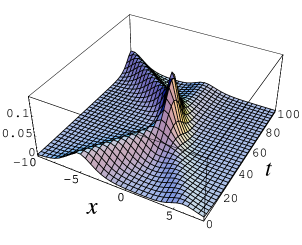
Figure 11: Evolution of the moduli variables and evolution of the lumps in the sector AO.

Back in the original coordinates, a typical $(a(t),b(t))$ geodesic is depicted in Figure 11 (left). The $b(t)$ curve shows that the relative distance between the two basic kinks decreases with time until they become fused -$b=0$- at $t=50$. Then, the distance starts to grow towards a complete splitting of the K${}_{1}^{AB}$ and K${}_{1}^{BO}$ kinks in the remote future. The evolution of the center of mass is unveiled by the $a(t)$ curve: it remains at $x=0$ while the two basic kinks are far apart. Shortly before the collision, $a$ starts to grow and thereafter continuous to increase. The two kinks rebound, the center of mass being closer to the heaviest kink. The picture is clearer in the plot of the energy density evolution along this geodesic shown in Figure 11 (right). Shortly after $t=-\infty$, the geodesic starts from a point in the moduli space corresponding to one K${}_{1}^{AB}$ kink and one K${}_{1}^{BO}$ kink very far apart. The two basic lumps begin to approach each other as $|b|$ decreases, distorting their shapes when they start to collide. Later, a single K${}_{2}^{AO}(0)$ lump is formed when $b(t)$ reaches $0$ (see Figures 5 and 11 (right)). At this point, the two lumps bounce back following the above-described motion in reverse, i.e., the separation between the two lumps increases, running asymptotically towards the configuration of two infinitely separated kinks in the ${\cal C}^{AO}_{\pm}$ sector. Thinking of the graphics in Figure 5 as the stills of a movie, the adiabatic dynamics of the double solitary waves prescribes the speed at which the film is played.

4.2 Meta-stable slow motion of quadruple solitary waves

We now perform the same analysis in the ${\cal C}^{BB}_{\pm\mp}$ sectors, again for the value $\sigma=\frac{1}{\sqrt{2}}$. The metric

$$h_{aa}(a,b)=2h_{bb}(a,b)=\frac{1}{2}$$

$$h_{ab}(a,b) = -\frac{1}{32}\left[10+\frac{e^{b}}{(e^{b}-1)^{\frac{3}{2}}}\left(\pi{\rm Sign}(e^{b}-1)-2{\rm arctan}\frac{1}{\sqrt{e^{b}-1}}\right)\right.$$

$$\left.-\frac{\sqrt{e^{b}}}{(1-e^{b})^{\frac{3}{2}}}\left(-\pi{\rm Sign}(1-e^{b})+2{\rm arctan}\frac{\sqrt{e^{b}}}{\sqrt{1-e^{b}}}\right)\right]$$

is of the general form studied in the previous sub-Section.

                   

Figure 12: Graphics from left to right of $h_{ab}$ and $h=h_{aa}h_{bb}-h_{ab}^{2}$ as functions of $b$.

The geodesics are easily found and plotted using Mathematica in Figure 13 (left). The evolution of the energy density along this geodesic is also shown in Figure 13 (right). The motion begins at $t=-\infty$ with three lumps very far away from each other along the real line , arranged as a K${}_{1}^{BO}$, K${}_{2}^{AO}$, K${}_{1}^{AB}$ configuration, ordered by increasing $x$. Then, the lumps start to approach the K${}_{2}^{AO}$ kink until they coincide, forming the K${}_{4}^{BB}(0)$ configuration. Later, the three lumps start to split in such a way that the K${}_{1}^{BO}$ kink overtakes the K${}_{2}^{AO}$ and K${}_{1}^{AB}$ lumps whereas the latter kink is also passed by the K${}_{2}^{AO}$ kink. This motion naturally proceeds towards K${}_{1}^{AB}$, K${}_{2}^{AO}$, K${}_{1}^{BO}$ configurations with growing distances between the basic lumps. Note that there are no problems in this sector at $b=\pm\infty$; contrarily to the $g$-metric the $h$-metric does not vanish at infinity. This means that some lumps could disappear smoothly as an effect of this low-energy scattering.

         

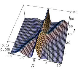
Figure 13: Evolution of the moduli variables and evolution of the lumps in the sector ${\cal C}^{BB}_{\pm\mp}$.

In fact, in Section §3 we argued that the K${}_{4}^{BB}$ solitary waves are unstable by demonstrating the existence of a negative eigenfunction of the Hessian. Fluctuations in this direction of the configuration space will destroy the gentle evolution between the solitary waves described above. Closer understanding of the non-adiabatic process triggered by the negative fluctuation is possible by starting from a K${}_{4}^{BB}(b)$ lump with large $b$: there are one K${}_{1}^{AB}$ and one K${}_{1}^{BO}$ lumps, respectively near $x=-\infty$ and $x=+\infty$, together with a K${}_{2}^{AO}$ kink sitting at the origin $x=0$. The zero mode

$$\psi_{\omega^{2}=0}^{(2)}=\frac{1}{\sqrt{{\rm cosh}(x-a)}}$$

of the Hessian at K${}_{2}^{AO}(0)$ provides a very good approximation to the negative eigenfunction of the Hessian at K${}_{4}^{BB}(b\rightarrow\infty)$ because this latter solitary wave tends asymptotically to K${}_{2}^{AO}(0)$, $\psi^{(0)}$ has no nodes, and the topological barriers in the ${\cal C}^{AO}_{\pm}$ and ${\cal C}^{BB}_{\pm\mp}$ sectors are different. Moreover, the $\psi^{(2)}_{0}$ fluctuation causes the splitting of the K${}_{2}^{AO}$ lump and the evolution reveals the motion of four lumps: two K${}_{1}^{AB}$ and two K${}_{1}^{BO}$ kinks. Of course, this configuration does not belong to the static kink family (28); the negative fluctuation suppresses the overlapping of two basic lumps.

This picture is confirmed by solving via numerical analysis the Cauchy problem for the PDE system (3)-(4) with initial conditions

$$\phi(x,0)={\rm K}_{4}^{AB}(30)(x)\qquad\qquad,\qquad\qquad\frac{\partial\phi}{\partial t}(x,0)=\varepsilon\psi^{(2)}_{0}(x)$$

and Dirichlet boundary conditions, see Figure 14. It seems that the two K${}_{1}^{BO}$ attract each other but there is repulsion between the two K${}_{1}^{AB}$ kinks.

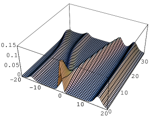
Figure 14: Evolution of a ${\rm K_{4}}^{BB}(b)$ solitary wave after $\psi^{(2)}_{0}$ fluctuations.

4.3 Perturbing the system: non-linear wave bound state

Finally, we add an small perturbation to our system. The basic kinks K${}_{1}^{BO}$ and K${}_{1}^{AB}$ move adiabatically along the geodesics of the metric induced by the kinetic energy on the kink moduli space in the ${\cal C}^{AO}_{\pm}$ sector. We choose to induce forces between the basic kinks by the following modification of $V(\phi_{1},\phi_{2})$:

$$V^{\prime}(\phi_{1},\phi_{2})=V(\phi_{1},\phi_{2})+\varepsilon v(\phi_{1},\phi_{2})\qquad,\qquad v(\phi_{1},\phi_{2})=\phi_{1}^{2}\left(\phi_{1}^{2}+\frac{\phi_{2}^{2}}{1-\sigma^{2}}-1\right)^{2}\qquad.$$

Here, $\varepsilon$ is an small parameter and our choice is such that the zeroes of $V$ are also zeroes of $V^{\prime}$; thus, $V^{\prime}$ also comply with Coleman’s theorem and enters into the class of admissible deformations of $V_{\rm CSH}$ in (1+1)-dimensions. Moreover, the K${}_{1}^{AB}$ and K${}_{1}^{BO}$ kinks survive this perturbation without any changes: they are still solitary wave solutions with the same energy. The K${}_{2}^{AO}$ solitary wave, however, needs to be adjusted:

$$\bar{\phi}(x,a)=(-1)^{\alpha}{1\over\sqrt{2}}\sqrt{1+(-1)^{\beta}{\rm tanh}[\sqrt{1+2\varepsilon}(x-a)]}\qquad,\quad\alpha,\beta=0,1\qquad,$$

is a solitary wave solution of the perturbed system with higher energy: ${\cal E}^{\prime}({\rm K_{2}}^{AO})={1\over 4}\sqrt{1+2\varepsilon}$. The perturbation is chosen in such a way that the kink energy sum rule (25) is broken.

All the other solitary wave are destroyed by the perturbation. Nevertheless, the adiabatic approximation can still be used to describe the slow motion of the basic lumps. For small enough $\varepsilon$, $\varepsilon<<1$, the solitary waves (24) are approximate solutions of the perturbed system; therefore, we take the parameters $a$ and $b$ as the moduli variables, even though the perturbation forbids neutral equilibria in the moduli space. Plugging the approximate solutions into the action of the perturbed model we obtain:

$$S^{G}=\int dt\left[\frac{1}{2}g_{aa}\frac{da}{dt}\frac{da}{dt}+g_{ab}\frac{da}{dt}\frac{db}{dt}+\frac{1}{2}g_{bb}\frac{db}{dt}\frac{db}{dt}-\varepsilon u(b)\right]\qquad.$$ (37)

The perturbation induces a potential energy, plotted in Figure 15 (left),

$$u(b)=\int_{-\infty}^{\infty}\,dx\,v({\rm K_{2}}^{AO}(b)(x))$$

and the motion ceases to be geodesic; $u(b)$ is a potential barrier with maximum height reached at $b=0$ that goes to zero for $b=\pm\infty$. The equations of motion coming from (37) determine the evolution of the moduli variables $a(t)$ and $b(t)$ with time.

In Figure 15 (center) the plot of both $a$ and $b$ as a function of time is shown for a solution of the equations of motion with $\varepsilon=0.1$ and initial conditions $a(0)=0$, $b(0)=-2.004$, $a^{\prime}(0)=0$, $b^{\prime}(0)=0.001$. The surprising outcome is that $b$ seems to be quasi-periodic in time; this is a Sisyphean movement, crossing over and over again the top of the hill!

In Figure 15 (right) the evolution of the energy density along this quasi-periodic orbit is drawn. We observe that the net effect of the perturbation plus the non-trivial metric is the upsurge of an attractive force between the two basic lumps K${}_{1}^{BO}$ and K${}_{1}^{AB}$, giving rise to a bound state similar to the breather mode in the sine-Gordon model.

     

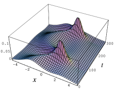
Figure 15: Plot of $u(b)$, evolution of the moduli variables and evolution of the lumps in the deformed model.

References

- [1]
- [2] J. Scott Russell, Report on waves, delivered to the Meetings of the Edinburgh Royal Society, 1843.
- [3] R. Rajaraman and E.J.Weinberg, “Internal symmetry and the semiclassical method in quantum field theory”, Phys. Rev. D 11 (1975) 2950.
- [4] R. Rajaraman, Solitons and instantons. An introduction to solitons and instantons in quantum field theory, North-Holland Publishing Co. 1987.
- [5] C. Montonen, “On solitons with an Abelian charge in scalar field theories: (I) Classical theory and Bohr-Sommerfeld quantization”, Nucl. Phys. B 112 (1976) 349-357.
- [6] S. Sarker, S. E. Trullinger and A. R. Bishop, “Solitary-wave solution for a complex one-dimensional field”, Phys. Lett. A 59 (1976) 255-258.
- [7] K. R. Subbaswamy and S. E. Trullinger, “Intriguing properties of kinks in a simple model with a two-component field”, Physica D 2 (1981) 379-388.
- [8] K. R. Subbaswamy and S. E. Trullinger, “Instability of non topological solitons of coupled scalar field theories in two dimensions”, Phys. Rev. D 22 (1980) 1495-1496.
- [9] E. Magyari and H. Thomas, “Solitary waves in a 1D anharmonic lattice with two-component order parameter”, Phys. Lett. A 100 (1984) 11-14.
- [10] H. Ito, “Kink energy sum rule in a two-component scalar field model of 1+1 dimensions”, Phys. Lett. A 112 (1985) 119-123.
- [11] H. Ito and H. Tasaki, “Stability theory for nonlinear Klein-Gordon Kinks and Morse’s index theorem”, Phys. Lett. A 113 (1985) 179-182.
- [12] J. Mateos Guilarte, A note on Morse theory and one-dimensional solitons, Lett. Math. Phys. 14 (1987) 169-176, “Stationary phase approximation and quantum soliton families”, Ann. Phys, 188 (1988) 307-346.
- [13] D. Bazeia, M. J. Dos Santos and R. F. Ribeiro, “Solitons in systems of coupled scalar fields”, Phys. Lett. A 208 (1995) 84-88.
- [14] D. Bazeia, J. R. S. Nascimento, R. F. Ribeiro and D. Toledo, “Soliton stability in systems of two real scalar fields”, J. Phys. A 30 (1997) 8157-8166.
- [15] M. Shifman and M. Voloshin, “Degenerate Domain Wall Solutions in Supersymmetric Theories”, Phys. Rev. D 57 (1998) 2590.
- [16] A. Alonso Izquierdo, M.A. Gonzalez Leon, J. Mateos Guilarte and M. de la Torre Mayado, “Kink variety in systems of two coupled scalar fields in two space-time dimensions”, Phys. Rev. D 65 (2002) 085012.
- [17] A. Alonso Izquierdo, M.A. Gonzalez Leon, J. Mateos Guilarte and M. de la Torre Mayado, “Adiabatic motion of two-component BPS kinks”, Phys. Rev. D 66 (2002) 105022.
- [18] A. Alonso Izquierdo, M. A. Gonzalez Leon, and J. Mateos Guilarte, “Kink manifolds in (1+1)-dimensional scalar field theory”, J. Phys. A: Math. Gen. 31 (1998), 209-229.
- [19] E. B. Bogomol’nyi, “The stability of classical solutions”, Sov. J. Nucl. Phys. 24 (1976) 449-454.
- [20] W. Garcia Fuertes and J. Mateos Guilarte, “On the solitons of the Chern-Simons-Higgs model”, Eur. Jour. Phys. C 9 (1999) 167-179.
- [21] S. Zhang, T. Hansson and S. Kivelson, “The Ginzburg-Landau theory for the fractionary quantum Hall effect”, Phys. Rev. Lett. 62 (1989) 82-85.
- [22] S. Coleman, “There are no Goldstone bosons in two dimensions”, Com. Math. Phys. 31 (1973) 259-264.
- [23] N. Manton, “A remark on the scattering of BPS monopoles”, Phys. Lett. B 110 (1982) 54-56.
- [24] P. L. Kapitsa, “Dynamic stability of a pendulum with oscillating suspension point”, Zh. Exper. Teor. Phys. 21 (1951) 588-598.
- [25] A. Alonso Izquierdo, M.A. Gonzalez Leon, J. Mateos Guilarte and M. de la Torre Mayado, “Supersymmetry versus integrability in two-dimensional classical mechanics”, Ann. Phys. 308, (2003) 664-691.