Random Delays and the Synchronization of Chaotic Maps

Abstract

We investigate the dynamics of an array of logistic maps coupled with random delay times. We report that for adequate coupling strength the array is able to synchronize, in spite of the random delays. Specifically, we find that the synchronized state is a homogeneous steady-state, where the chaotic dynamics of the individual maps is suppressed. This differs drastically from the synchronization with instantaneous and fixed-delay coupling, as in those cases the dynamics is chaotic. Also in contrast with the instantaneous and fixed-delay cases, the synchronization does not dependent on the connection topology, depends only on the average number of links per node. We find a scaling law that relates the distance to synchronization with the randomness of the delays. We also carry out a statistical linear stability analysis that confirms the numerical results and provides a better understanding of the nontrivial roles of random delayed interactions.

A system composed of many nonlinear interacting units often forms a complex system with new emergent properties that are not held by the individual units. Such systems describe a wide variety of phenomena in biology, physics, and chemistry. The emergent property is usually synchronous oscillations. In biology examples are the synchronized activity in pacemaker heart cells, the cicardian rhythms that control 24h daily activity, and the flashing on-and-off in unison of populations of fireflies. Nonbiological examples include synchronized oscillations in arrays of electrochemical reactions, in laser arrays, and in Josephson junction arrays reviews .

The effect of time-delayed interactions, which arise from a realistic consideration of finite communication times, is a key issue that has received considerable attention. The first systematic investigation of time-delayed coupling was done by Schuster and Wagner schuster_PTP_1989 , who studied two coupled phase oscillators and found multistability of synchronized solutions. Since then, delayed interactions have been studied in the context of linear systems jirsa_PRL_2004 , phase oscillators phase_osc , limit-cycle oscillators limit_cycl , coupled maps maps ; atay_PRL_2004 , neuronal neuronal ; misha ; longtin and laser laser systems. Most studies have assumed that all the interactions occur with the same delay time (only few have consider non-uniform delays longtin ; zanette_PRE_2000 ; marti ). However, actual delays in real extended systems are not necessarily the same for all the elements of the system, they might be distant-dependent or randomly distributed. In populations of spatially separated neurons, the synaptic communications between them, which depend on the propagation of action potentials over appreciable distances, involve distributed delays. In computer networks, random delays arise from queueing times and propagation times. In epidemic dynamics, migrations of geographically spread populations lead to different delays which influence the transmission of diseases.

While it is well-known that oscillators which interact with different delay times can synchronize (an example is the synchrony arising in different neuronal groups of the brain which might lead to both, epilepsy and Parkinson disease), the mechanism by which this synchrony arises and the influence of the random communication times remains poorly understood. The focus of this letter is to investigate the influence of such random delays in the synchronization of a simple model of coupled chaotic oscillators. We consider an ensemble of logistic maps and show that, in spite of the random delays, for adequate coupling strength the array is able to synchronize. Surprisingly, in the synchronized state the chaotic dynamics of the individual maps is suppressed: the maps are in a steady-state, which is unstable for the uncoupled maps. This is in sharp contrast with the cases of instantaneous and fixed-delay coupling, as in those cases the dynamics of the array is chaotic. By studying the transition from chaotic synchronization to steady-state synchronization as the randomness of the delays increases we discover a scaling law that relates the distance to synchronization with the randomness of the delays. We also investigate the influence of the array topology and find that steady-state synchronization depends on the average number of links per node but not on the array architecture. This is also in contrast with the instantaneous and fixed-delay cases, as in those cases the synchronization depends also on the connection topology atay_PRL_2004 . Finally, we present a statistical linear stability analysis that demonstrates the stability of the solution found numerically.

We consider the following ensemble of $N$ coupled maps:

$$x_{i}(t+1)=(1-\epsilon)f[x_{i}(t)]+\frac{\epsilon}{b_{i}}\sum_{j=1}^{N}\eta_{ij}f[x_{j}(t-\tau_{ij})]$$ (1)

Here $t$ is a discrete time index, $i$ is a discrete spatial index ($i=1\dots N$), $f(x)=ax(1-x)$ is the logistic map, the matrix $\eta=(\eta_{ij})$ defines the connectivity of the array: $\eta_{ij}=\eta_{ji}=1$ if there is a link between the $i$th and $j$th nodes, and zero otherwise. $\epsilon$ is the coupling strength and $\tau_{ij}$ is the delay time in the interaction between the $i$th and $j$th nodes (the delay times $\tau_{ij}$ and $\tau_{ji}$ need not be equal). The sum in Eq.(1) runs over the $b_{i}$ nodes which are coupled to the $i$th node ($b_{i}=\sum_{j}\eta_{ij}$). The normalized pre-factor $1/b_{i}$ means that each map receives the same total input from its neighbours.

First we note that the homogeneous steady-state $x_{i}(t)=x_{j}(t)=x_{0}$, $\forall$ $i$, $j$, $t$, where $x_{0}$ is a fixed point of the uncoupled map, $x_{0}=f(x_{0})$, is a solution of Eq.(1) regardless of the delays and of the connectivity of the array.

Next, let us present some results of simulations that show that this state, with $x_{0}$ being the nontrivial fixed point, $x_{0}=1-1/a$, can be a stable solution for adequate coupling and random enough delays. The simulations were done choosing an initial configuration, $x_{i}(0)$ random in [0,1], and letting the array evolve initially without coupling [in the first time interval $0<t<\max(\tau_{ij})$]. We present results for $a=4$, corresponding to fully developed chaos of the individual maps, but we have found similar results for other values of $a$. We illustrate our findings using the small-world topology nw_1999 , but we have found similar results for random and regular topologies nota1 , as discussed below.

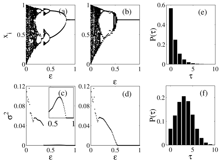
Figure 1: $x_{i}$ vs. $\epsilon$ (a) and (b); $\sigma^{2}$ vs. $\epsilon$, (c) and (d). In Figs. 1(a) and 1(c) the delays are distributed exponentially ($\tau_{0}=0$, $c=1.2$, see text); the distribution is shown in Fig. 1(e). In Figs. 1(b) and 1(d) the delays are Gaussian distributed ($\tau_{0}=3$, $c=2$, see text); the distribution is shown in Fig. 1(f). The inset in Fig. 1(d) shows with detail the transition to synchronization: $\sigma^{2}$ decreases abruptly at $\epsilon\sim 0.4$, and is zero for $\epsilon>0.8$. Parameters are: $N=500$, $a=4$, and $p=0.3$.

With both, either randomly distributed or fixed delay times, if the coupling is large enough the array synchronizes in a spatially homogeneous state: $x_{i}(t)=x_{j}(t)$ $\forall$ $i,j$. Figures 1 and 2 display the transition to synchronization as $\epsilon$ increases. At each value of $\epsilon$, 100 iterates of an element of the array are plotted after transients. To do the bifurcation diagrams we varied only $\epsilon$; the connectivity of the array ($\eta_{ij}$), the delays ($\tau_{ij}$), and the initial configuration [$x_{i}(0)$] are the same for all values of $\epsilon$. Figure 1(a) displays results for delays that are exponentially distributed, Fig. 1(b) for Gaussian distributed, Fig. 2(a) for zero delay, and Fig. 2(b) for constant delays. It can be observed that for small $\epsilon$ the four bifurcation diagrams are similar; however, for large $\epsilon$ they differ drastically: $x_{i}$ is constant in Figs. 1(a) and 1(b), $x_{i}=x_{0}=1-1/a$, while $x_{i}$ varies within [0,1] in Figs. 2(a) and 2(b).

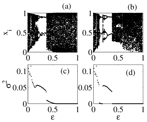
Figure 2: $x_{i}$ vs. $\epsilon$ (a) and (b); $\sigma^{2}$ vs. $\epsilon$ (c) and (d). In (a),(c) $\tau_{ij}=0$ $\forall$ $i$,$j$; in (b),(d) $\tau_{ij}=3$ $\forall$ $i$,$j$. All other parameters as in Fig. 1.

To characterize the transition to synchronization we use the indicator $\sigma^{2}=1/N<\sum_{i}[x_{i}(t)-<x>]^{2}>_{t}$, where $<.>$ denotes an average over the elements of the array and $<.>_{t}$ denotes an average over time. Figures 1(c), 1(d), 2(c) and 2(d) display $\sigma^{2}$ vs. $\epsilon$ for the bifurcation diagrams discussed above. It can be observed that for large $\epsilon$ there is inphase synchronization in the four cases [$x_{i}(t)=x_{j}(t)$ and $\sigma^{2}=0$]; however, we remark that an inspection of the time-dependent dynamics reveals that for randomly distributed delays the maps are in a steady-state, while for fixed delays the maps evolve chaotically. It can also be observed that the four plots $\sigma^{2}$ vs. $\epsilon$ are similar for small $\epsilon$ (in Fig. 2(d) the array synchronizes also in a window of small $\epsilon$; this occurs for odd delays and was reported in atay_PRL_2004 ).

Let us now investigate the transition from chaotic synchronization (for fixed delays) to steady-state synchronization (for random delays) by introducing a disorder parameter $c$ that allows varying the delays from constant to distributed values. Specifically we consider

i) $\tau_{ij}=\tau_{0}+\mathrm{Near}(c\xi)$, where $\xi$ is Gaussian distributed with zero mean and standard deviation one and $Near$ denotes the nearest integer. The delays are constant ($\tau_{ij}=\tau_{0}$) for $c=0$ and are Gaussian distributed around $\tau_{0}$ for $c\neq 0$ [depending on $\tau_{0}$ and $c$ the distribution of delays has to be truncated to avoid negative delays, see Fig. 1(f)].

ii) $\tau_{ij}=\tau_{0}+\mathrm{Int}(c\xi)$, where $\xi$ is exponentially distributed, positive, with unit mean and $Int$ denotes integer. The delays are constant ($\tau_{ij}=\tau_{0}$) for $c=0$ and are exponentially distributed, decaying from $\tau_{0}$ for $c\neq 0$.

Figure 3(a) displays the transition between the two synchronization regimes as the randomness of the delays increases. We plot $\sigma^{2}$ vs. $c$ for different delay time distributions and $\epsilon$ large enough such that the array synchronizes for $c=0$. It can be observed that the array desynchronizes as $c$ increases and the delays become different from each other. There is a range of values of $c$ such that the delays are not random enough to induce steady-state synchronization; however, for $c$ large enough the array synchronizes again and $\sigma^{2}=0$.

To investigate this transition we considered a normalized disorder parameter $c^{*}=D_{\tau}/<\tau>$, where $<\tau>$ is the average delay and $D_{\tau}$ is the standard deviation of the delay distribution. By plotting $\sigma^{2}$ vs. $c^{*}$ [Figs. 3(b)] we uncover a scaling law: as $<\tau>$ increases the curves collapse into curves of similar shape, and the transition to steady-state synchronization occurs for $c^{*}\sim 0.5$.

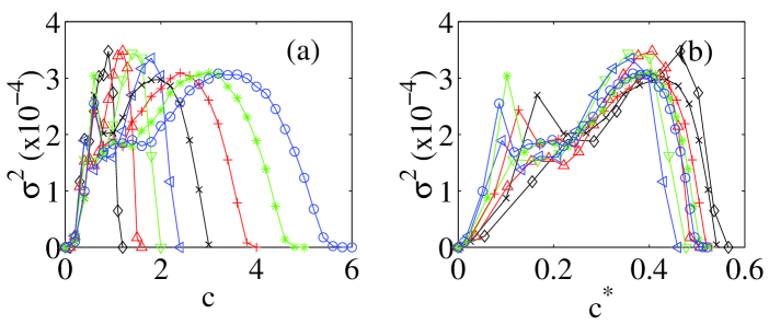
Figure 3: (a) $\sigma^{2}$ vs. $c$ and (b) $\sigma^{2}$ vs. $c^{*}$. The delays are Gaussian distributed with $\tau_{0}=2$ ($\diamond$), 3 ($\triangle$), 4 ($\nabla$), 5 ($\triangleleft$) ; exponentially distributed with $\tau_{0}=3$ ($\times$), 4 ($+$), 5 ($\ast$), 6 ($\circ$). $\epsilon=1$, all other parameters are as in Fig. 1.

The value of the disorder parameter above which the arrays synchronizes in the steady-state depends on the coupling strength. Figure 4(a) displays the synchronization region in the parameter space $(\epsilon,c)$. To determine the synchronization region we did simulations with different initial conditions, array connectivities, and delay time realizations: the black indicates parameters for which the array synchronized in all the simulations, while the white indicates parameters for which the array did not synchronize in any of the simulations. The grey region in the boundary of the synchronization region indicates that there are some initial conditions and/or realizations of $\eta_{ij}$ and $\tau_{ij}$ for which the array did not synchronize. Two different synchronization regions can be clearly distinguished: for $c=0$ and for $c>0.5$. The former corresponds to chaotic synchronization for fixed delays, and the latter, to steady-state synchronization for distributed delays.

Atay et al. atay_PRL_2004 have recently shown that with fixed delays the synchronization depends on the array architecture: with the same total number of links, a random network exhibits better synchronization properties than a regular network. We investigated this issue in the case of distributed delays and found that the synchronization depends on the average number of links per node, $<b_{i}>$, but not on the architecture. We did simulations with arrays of different topologies nota1 and found that the transition to synchronization is similar for all the arrays provided that they have the same $<b_{i}>$. Figure 5(a) displays the transition to synchronization as $\epsilon$ increases for small-world and regular arrays with distributed delays, and for comparison, Fig. 5(b) displays results for the same arrays with fixed-delays. It can be observed that for distributed delays the transition to synchronization is independent of the array topology; however, it depends on the connectivity: the larger the number of mean links per node, the lower the coupling strength needed synchronize. In contrast, for fixed delays the synchronization depends not only on the connectivity but also on the architecture: for $\epsilon$ large enough the arrays that have small-world topologies synchronize, but those that have regular topologies do not, in agreement with the results of atay_PRL_2004 .

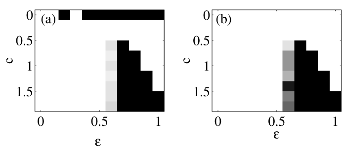
Figure 4: (a) Synchronization region determined numerically: black represents parameters where $\sigma^{2}<10^{-7}$ for all the realizations of $x_{i}(0)$, $\eta_{ij}$ and $\tau_{ij}$. (b) Synchronization region determined from the stability analysis: black represents parameters where the $|\lambda_{max}|<1$ for all the realizations of $\eta_{ij}$ and $\tau_{ij}$. The delays are Gaussian distributed with $\tau_{0}=3$, $N=100$, all other parameters are as in Fig. 1.

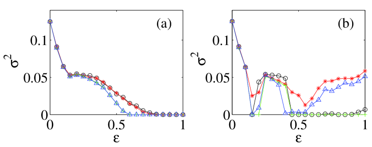
Figure 5: Influence of the architecture and the connectivity of the array for (a) Gaussian distributed delays ($\tau_{0}=3$, $c=2$) and (b) fixed delays ($\tau_{ij}=3$ $\forall$ $i$,$j$). Small-world topology with and an average of 10 links per node ($\circ$), 50 links per node (+); regular topology with 10 links per node (*); 50 links per node ($\triangle$). All other parameters are as in Fig. 1.

Finally, let us assess the stability of the steady-state synchronized behavior found numerically by performing a statistical linear stability analysis. The delayed map Eq. (1) can be written in non-delayed form by the introduction of a set of auxiliary variables marti , $y_{im}(t)=x_{i}(t-m)$, where $1\leq i\leq N$ and $0\leq m\leq M$ with $M=\max(\tau_{ij})$. In terms of these new $N(M+1)$ variables Eq. (1) becomes

$$y_{im}(t+1)=$$

$$\begin{cases}y_{i,m-1}(t)&\text{if $m\neq 0$},\\ (1-\epsilon)f[y_{i0}(t)]+\sum_{j=1}^{N}\epsilon_{ij}f[y_{j,\tau_{ij}}(t)]&\text{if $m=0$}.\end{cases}$$ (2)

Next we define a vector of $N(M+1)$ components containing information about the present and past states of the array (for $i=1$ to $N$ and for time $t$ to $t-M$): $Y=(y_{10},y_{20},\dots,y_{N0};y_{11},y_{21},\dots,y_{N1};\dots;y_{1M},y_{2M}\dots,y_{NM})$. Eq. (Random Delays and the Synchronization of Chaotic Maps) can be re-written as $Y_{i}(t+1)=F_{i}(Y_{1}(t)\dots Y_{N(M+1)}(t))$ and the synchronized state can be re-written as $Y^{*}=(x_{0}\dots x_{0}).$

Linearizing the equations of motion near $Y^{*}$ gives $\delta Y_{i}(t)=\sum_{j}f_{ij}\delta Y_{j}(t)$, where the matrix ${\bf F}=(f_{ij})$ with $f_{ij}=\partial F_{i}/\partial Y_{j}$ can be cast as a set of $(M+1)^{2}$ blocks of dimension $N\times N$. We denote these blocks as $\mathcal{F}_{kl}$, with $k,l=0,...M$. The blocks $\mathcal{F}_{kl}$ with $k>0$ have all components equal to $0$, except the blocks $\mathcal{F}_{k+1,k}$ which are $N\times N$ identity matrices. The elements of the blocks $\mathcal{F}_{kl}$ with $k=0$ can be considered as composed by two parts: (i) $(1-\epsilon)f^{\prime}(x_{0})$, which arise from the non-delayed term in Eq. (1) and appear in the diagonal of $\mathcal{F}_{00}$. (ii) $(\epsilon/b_{i})f^{\prime}(x_{0})$, which represent the contribution of a link and due to the random delays appear in random positions of the blocks. Each link contributes with two terms of the form $(\epsilon/b_{i})f^{\prime}(x_{0})$. There is a total of $2\sum_{i}b_{i}$ terms $(\epsilon/b_{i})f^{\prime}(x_{0})$ are which are distributed randomly in the blocks $\mathcal{F}_{0l}$. More precisely, they are located at the positions $(i,j)$ and $(j,i)$ in the blocks $\mathcal{F}_{0\tau_{ij}}$ and $\mathcal{F}_{0\tau_{ji}}$ respectively. The rest of the elements are zero.

We calculated the eigenvalues of ${\bf F}$ for different realizations of the connectivity and delay time distributions. The results are displayed in Fig. 4(b), where the black region indicates parameters where the maximum eigenvalue of $\bf{F}$, $\lambda_{max}$, has modulus less than 1 for all $\tau_{ij}$ and $\eta_{ij}$ realizations, and the white region indicates parameters where $\lambda_{max}\geq 1$ for all $\tau_{ij}$ and $\eta_{ij}$ realizations. A very good agreement with the synchronization region determined numerically can be observed [the black region for $c=0$ observed in Fig. 4(a) does not appear in Fig. 4(b) because in this region the synchronized dynamics is chaotic].

To conclude, we studied the dynamics of an ensemble of chaotic maps which interact with random delay times, and found that for adequate coupling strength the array synchronizes with all the maps in a steady-state. The synchronization is independent of the architecture of the array, but depends on the average number of links per node. We confirmed the numerical results by performing a statistical linear stability analysis. Our findings provide another example of the nontrivial action of inhomogeneities and disorder in coupled nonlinear systems; in our case, the presence of large enough disorder in the interaction times plays a constructive role, suppressing the chaotic dynamics of the individual units. We speculate that the ”chaos-suppression by random delays” reported here might yield light into explaining the stable operation of many complex systems composed by nonlinear units which interact with each other with random communication times.

References

- (1) A.S. Pikovsky, M.G. Rosenblum, and J. Kurths, Synchronization- A Universal Concept in Nonlinear Sciences (Cambridge University Press, Cambridge, England, 2001); Y. Kuramoto, Chemical Oscillations, Waves, and Turbulence (Springer-Verlag, Berlin, 1984); S. Bocaletti et al., Physics Reports 366, 1 (2002); L.M. Pecora et al., Chaos 7, 520 (1997).
- (2) H. G. Schuster and P. Wagner, Prog. Theo. Phys. 81, 939 (1987).
- (3) V. K. Jirsa, and M. Ding, Phys. Rev. Lett. 93, 070602 (2004).
- (4) E. Niebur et al., Phys. Rev. Lett. 67 2753 (1991); Ernst et al., Phys. Rev. Lett. 74, 1570 (1995); S. Kim et al., Phys. Rev. Lett. 79, 2911 (1997); M. K. Stephen Yeung and S. H. Strogatz, Phys. Rev. Lett. 82, 648 (1999); M. G. Earl and S. H. Strogatz, Phys. Rev. E 67, 036204 (2003); M. Denker et al., Phys. Rev. Lett. 92, 074103 (2004).
- (5) D. V. Ramana Reddy et al., Phys. Rev. Lett. 80, 5109 (1998); D. V. Ramana Reddy et al., Phys. Rev. Lett. 85, 3381 (2000); R. Dodla et al., Phys. Rev. E 69, 056217 (2004).
- (6) Y. Jiang, Phys. Lett. A 267, 342 (2000); C. Li et al., Physica A 335, 365 (2004).
- (7) F. M. Atay et al., Phys. Rev. Lett. 92, 144101 (2004).
- (8) R. Herrero et al., Phys. Rev. Lett. 84, 5312 (2000); A. Takamatsu et al., Phys. Rev. Lett. 85, 2026 (2000); A. Takamatsu et al., Phys. Rev. Lett. 87, 078102 (2001); Phys. Rev. Lett. 92, 228102 (2004); M. Dhamala et al., Phys. Rev. Lett. 92, 074104 (2004).
- (9) M. Rosemblum and A. Pikovsky, Phys. Rev. Lett. 92, 114102 (2004); Phys. Rev. E 70, 041904 (2004).
- (10) B. Doiron et al., Phys. Rev. Lett. 93, 048101 (2004).
- (11) J. García-Ojalvo et al., Int. J. Bifurcation Chaos 9, 2225 (1999); G. Kozyreff et al., Phys. Rev. Lett. 85, 3809 (2000); A. G. Vladimirov et al., Europhys. Lett., 61, 613 (2003).
- (12) D. H. Zanette, Phys. Rev. E. 62, 3167 (2000); S. O. Jeong et al., Phys. Rev. Lett. 89, 154104 (2002); T. W. Ko et al., Phys. Rev. E 69, 056106 (2004); F. M. Atay, Phys. Rev. Lett. 91, 094101 (2003).
- (13) A. C. Martí and C. Masoller, Phys. Rev. E 67, 056219 (2003).
- (14) M. E. J. Newman and D. J. Watts, Phys. Rev. E 60, 7332 (1999); Phys. Letts. A 263, 341 (1999).
- (15) To built a small-world topology we begin with a circular chain of nodes and add with probability a link between two nodes ( corresponds to a circular array with nearest-neighbour coupling, corresponds to a globally coupled array); to built a random topology we begin with nodes and add with probability () a link between two nodes; to built a regular topology we begin with nodes and couple each node with its nearest neighbors.
- (16) Unfortunatelly, we were not able to investigate system size effects because of the large memory requirements needed to simulate large arrays with delayed coupling. To the best of the numerical resolution we have not observed significant differences in the synchronization of arrays with small-world, random and regular topologies, as long as the average number of links per node, , is equal. The results of the stability analysis confirm this numerical prediction.