Solitary Wave Interactions In Dispersive Equations Using Manton’s Approach

Abstract

We generalize the approach first proposed by Manton [Nuc. Phys. B 150, 397 (1979)] to compute solitary wave interactions in translationally invariant, dispersive equations that support such localized solutions. The approach is illustrated using as examples solitons in the Korteweg-de Vries equation, standing waves in the nonlinear Schrödinger equation and kinks as well as breathers of the sine-Gordon equation.

Introduction. Dispersive wave nonlinear partial differential equations (PDEs) describe a variety of physical systems in atomic, optical, molecular, solid state and wave physics as well as in fluid dynamics, biophysics, plasma physics, high energy physics and astrophysics among others [2, 3]. Often in these settings, it is of particular interest to examine the dynamics and interactions of spatially localized, and possibly travelling in time, solutions which can represent bits of information, moving Bose-Einstein condensates, elementary particles or water waves [4, 5]. Particularly the interactions between the solitary waves are especially important, since, e.g., in optical communications avoiding such interactions may reduce the bit error rate [6]; in Bose-Einstein condensates such interactions change significantly the form of the wavefunction [7], while in high energy physics models, the interactions are used to monitor the collisions of elementary particles [8].

There is a vast amount of literature regarding the interactions and collisions of the above mentioned solitary waves. Many reviews of continuum [9, 10] and discrete [11] systems contain some of this enormous volume of work. The techniques that have been used to identify the nature of such interactions are also rather diverse ranging from perturbation theoretic ones as, e.g., in the work of Ref. [12], to variational ones [10, 13, 14], to more rigorous ones, using the Fredholm alternative [15] or Lin’s method as in Ref. [16]. Typically, these interactions asymptotically follow the tails of the waves, which in most cases are exponential. This, in turn, results in writing down Toda lattice type equations at the “mesoscopic” level for lattices of coherent nonlinear waves, see, e.g., Refs. [14, 17] and references therein.

While the solitary wave interactions have been extensively studied in the past, in the present communication we aim at presenting a different viewpoint on this topic. Our aim, in particular, is to explicitly focus on calculating the tail-tail interactions between the waves, using the method proposed by Manton in Ref. [18], based on the earlier work of Refs. [19, 20, 21] and systematize it as a general method that can be straightforwardly applied to any nonlinear dispersive wave equation that has a number of characteristics (which will be analyzed/explained). We believe that this method provides a very simple, yet elegant and useful tool that can be generically used in this large class of models and hence would be of value to researchers in a variety of disciplines.

The structure of our presentation is as follows: initially we repeat Manton’s formulation for the kink-antikink interaction in the sine-Gordon equation, highlighting some key and subtle points. We then proceed to an analogous calculation for the case of solitons in the Korteweg-de Vries (KdV) equation. We then move to the realm of breathers starting with the standing waves (with trivial periodicity) in the case of the nonlinear-Schrödinger (NLS) equation. Thereafter, we study the interaction of genuinely breathing structures such as the breathers of the sine-Gordon equation. All of our results are corroborated with numerical simulations. Finally, we conclude our presentation with a summary of main findings and some intriguing questions for future study.

Manton’s Formulation for sine-Gordon Kinks. At the heart of Manton’s calculation of the interaction energy is the use of the definition of the linear momentum of the wave equation at hand. Computing the time derivative of the momentum $P$ for an interval containing one solitary wave, and deducing the contribution to it from the second wave, we can infer the force exerted on the soliton from its neighbor. In particular, for Lorentz-invariant equations (e.g. Klein-Gordon equations) of the form:

$$u_{tt}=u_{xx}-V^{\prime}(u),$$ (1)

the linear momentum can be written as:

$$P=-\int u_{t}u_{x}dx.$$ (2)

The total integral along the line is a conserved quantity (when the model is translationally invariant, an assumption necessary for this approach to work). Consider a soliton centered around $\xi=0$ ($u^{(1)}$), and an antisoliton centered at $\xi=\Delta\xi$ ($u^{(2)}$), then using an interval $(a,b)$ such that $a\ll 0$ and $0\ll b\ll\Delta\xi$, we find that in that interval (as shown in Ref. [18]):

$$\frac{dP}{dt}=\left[-u_{x}^{(1)}u_{x}^{(2)}+u_{xx}^{(1)}u^{(2)}\right]_{a}^{b}.$$ (3)

If we then take into account the asymptotic form of the kink-like waves, which for $V(u)=1-\cos(u)$ are of the form $u=4\arctan(e^{\pm x})$, we find that $u^{(1)}\approx 4\exp(-x)$ and $u^{(2)}\approx 4\exp(-(x-\Delta\xi))$ in the region between the solitons (and hence at $x=b$). At $x=a$ the contribution will be null as $a\rightarrow-\infty$. Manton’s end result is thus:

$$\frac{dP}{dt}=32\exp(-\Delta\xi),$$ (4)

(which is independent of b) and hence the potential of interaction is $V(\Delta\xi)=-32\exp(-\Delta\xi)$.

There are some subtleties here that we would like to highlight:
$\bullet$ Notice that $dP/dt=\partial V/\partial\Delta\xi$ has been used in the derivation of the potential, as opposed to the usual $(-)$ sign on the right hand side. This is because, the way the momentum is defined, $dP/dt>0$ which means that the momentum at $x=b$ is increasing, which in turn means that the solitary wave is approaching $x=b$, because of the interaction and hence $\Delta\xi$ is decreasing (i.e., when $dP/dt>0$, the resulting force in the dynamics of $\Delta\xi$ is negative). This sign change accounts for the above formula used in the derivation of the potential. This subtle point should always be taken into consideration when using Manton’s method.
$\bullet$ Secondly, if we are to examine the dynamics of $\Delta\xi$, then the corresponding Newton equation should account not only for the potential, but also for the “mass” of the solitary wave. In the case at hand (kinks of the sine-Gordon equation), the mass $M=\int u_{x}^{2}dx=\int\left[\frac{1}{2}u_{x}^{2}+(1-\cos(u))\right]$ is $8$.
$\bullet$ Finally, for the dynamical equation of $\Delta\xi$, we should take into consideration that we have only computed the force on the “left soliton” from the right one. However, there is an equal and opposite force on the right solitary wave and hence we should use a factor of $2$ when writing the equation for the acceleration of $\Delta\xi$.
Incorporating all these points in the equation for the separation between the solitary waves we obtain that, Manton’s formulation yields in general:

$$\ddot{\Delta\xi}=-\frac{2}{M}\frac{dP}{dt},$$ (5)

where the overdot denotes temporal derivative. In the particular case of sine-Gordon kink-antikink interaction, Eq. (5) yields

$$\ddot{\Delta\xi}=-8\exp\left(-\Delta\xi\right)\,.$$ (6)

A numerical example illustrating/validating the usefulness of this formula is given in Fig. 1. It is worth remarking here that for all Lorentz-invariant theories, while the kink-antikink interaction is attractive, the kink-kink interaction is always repulsive.

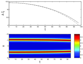
FIG. 1.: Kink-antikink attractive interaction in the sine-Gordon equation. The kinks are initialized at a distance of $\approx 10.4$ and are allowed to interact. The top panel shows their separation (numerically measured using a local center of mass approach weighted on the energy density) as a function of time. The solid line shows the numerical result, while the dashed one indicates the result of integrating Eq. (6). The bottom panel shows the space-time (x-t) contour plot of the energy density, indicating the tendency of the waves to approach each other.

Soliton Interaction in the KdV Equation. Another interesting example that illustrates some additional subtleties of the Manton approach concerns the solitary wave interactions in the KdV equation (most often associated with water waves [4, 5]). Following the same path as above, the definition of momentum in this case is given by $P=\int u^{2}dx$, hence we compute $dP/dt$. Given the form of KdV (in travelling wave frame with velocity C):

$$u_{t}=-u_{xxx}-6uu_{x}+Cu_{x}\,,$$ (7)

we find that

$$\frac{dP}{dt}=2\int_{a}^{b}uu_{t}=\left[4u^{3}-2uu_{xx}+u_{x}^{2}+Cu^{2}\right]_{a}^{b}.$$ (8)

For a two-soliton decomposition $u=u^{(1)}+u^{(2)}$ and neglecting (exponentially smaller) higher order terms, we obtain the expression:

$$\frac{dP}{dt}\approx 2u_{x}^{(1)}u_{x}^{(2)}-2(u^{(1)}u_{xx}^{(2)}+u^{(2)}u_{xx}^{(1)})+2Cu^{(1)}u^{(2)}\,.$$ (9)

Finally, given the form of the soliton $u=(C/2){\rm sech}^{2}(\sqrt{C}x/2)$, the expression of Eq. (9) is evaluated as:

$$\frac{dP}{dt}=-16C^{3}\exp\left(-\sqrt{C}\Delta\xi\right).$$ (10)

Using the expression of Eq. (5), we would be immediately inclined to write (given that the mass of the soliton is $\int udx=2\sqrt{C}$)

$$\ddot{\Delta\xi}=16C^{5/2}\exp\left(-\sqrt{C}\Delta\xi\right).$$ (11)

However, we argue that when following Manton’s formalism, one should respect Ehrenfest’s theorem. In particular, in the case of KdV, it is true that:

$$\frac{d}{dt}\int xudx=3P\Rightarrow\frac{d^{2}}{dt^{2}}\int xudx=3\frac{dP}{dt}.$$ (12)

The left hand side indeed evaluates to $M\ddot{\Delta\xi}$ here (as well as for sine-Gordon), however the right hand side should be multiplied by a factor of 3. Hence, the resulting dynamical equation for the evolution of the soliton displacement should read:

$$\ddot{\Delta\xi}=48C^{5/2}\exp\left(-\sqrt{C}\Delta\xi\right).$$ (13)

A numerical example of the dynamics of KdV solitons is given in Fig. 2.

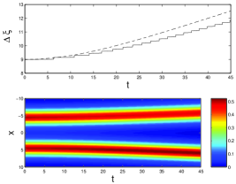
FIG. 2.: The (repulsive) two-soliton interaction in the KdV equation. The two panels are similar to those of Fig. 1. The small jumps in the top panel are due to the discretization used to emulate the continuum equation. The two solitons are initialized at a distance of $\Delta\xi=9$. The bottom panel shows the space-time (x-t) contour plot of the field $u$.

Standing Wave Interaction in the NLS Equation. In the case of the NLS equation (a model relevant predominantly to nonlinear optics and plasma physics [6], but also more recently to atomic physics as well [3]), the role of the mass is played by the squared $L^{2}$ norm, hence mass and momentum are defined as follows:

$$M=\int|u|^{2}dx;\hskip 14.22636ptP=\frac{i}{2}\int(uu_{x}^{\star}-u^{\star}u_{x})dx,$$ (14)

for the dynamical equation:

$$iu_{t}=-\frac{1}{2}u_{xx}-|u|^{2}u.$$ (15)

We can then compute similarly as above (up to higher order exponentially smaller terms):

$$\frac{dP}{dt}=\frac{1}{4}\left[uu_{xx}^{\star}+u_{xx}u^{\star}-2|u_{x}|^{2}\right]_{a}^{b}.$$ (16)

We again use the standard 2-soliton decomposition, $u=u^{(1)}+u^{(2)}$ where $u^{(1)}=\eta{\rm sech}(\eta x)\exp(i\eta^{2}t/2)$, $u^{(2)}=\eta{\rm sech}(\eta(x-\Delta\xi))\exp(i\eta^{2}t/2)\exp(i\phi)$ are the standing waves, and the relative phase $\phi$ between them has been incorporated in $u_{2}$. Then, one obtains:

$$\frac{dP}{dt}=8\eta^{4}\exp\left(-\eta\Delta\xi\right),$$ (17)

which results in the dynamical equation for the separation (using Eq. (5)) of the form:

$$\ddot{\Delta\xi}=-8\eta^{3}\exp\left(-\eta\Delta\xi\right)\cos\phi\,.$$ (18)

This equation is identical to the one obtained in [22] through variational and perturbation techniques [cf. Eq. (5) of [22]].

We have also examined numerically the validity of the results. A typical computation is summarized in Fig. 3. Notice that in the case of solitons in phase, the interaction is attractive while it is repulsive when the solitons are ($\pi$) out of phase. This is also observed in the numerical experiments.

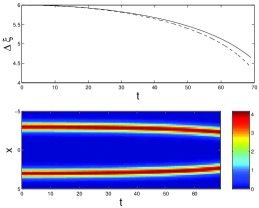
FIG. 3.: Same as in Fig. 1, but for the (in phase) standing waves of the NLS equation. The latter were initialized at a distance of 6. The bottom panel shows the space-time contour plots of the square modulus of the wavefunction $u$.

Breather Interaction in the sine-Gordon Equation. In the above examples we established cases where the interaction between the solitary waves was previously known and used them to analyze some of the key technical points of the Manton approach. We now turn to an example that, to the best of our knowledge, has not been treated analytically before and which concerns, in particular, the breather-breather interaction in the sine-Gordon equation. Such solutions of Eq. (1) are given by the form:

$$u=4\arctan\left[\frac{\sqrt{1-\omega^{2}}}{\omega}\sin(\omega t){\rm sech}\left(\sqrt{1-\omega^{2}}x\right)\right],$$ (19)

where $\omega$ is the breather frequency. A fundamental difference in this case is that the solutions are genuinely time dependent. However, the Manton formulation can still be carried through with the corresponding momentum derivative evaluated as:

$$\frac{dP}{dt}=\left[-u_{t}^{(1)}u_{t}^{(2)}-u_{x}^{(1)}u_{x}^{(2)}+(u_{xx}^{(1)}-u_{tt}^{(1)})u_{2}\right]_{a}^{b}.$$ (20)

As a result of the decomposition $u=u^{(1)}+u^{(2)}$ and the asymptotics $u^{(1)}\approx 8\sqrt{1-\omega^{2}}\sin(\omega t)\exp\left(-\sqrt{1-\omega^{2}}x\right)/\omega$ and $u^{(2)}\approx 8\sqrt{1-\omega^{2}}\sin(\omega t)\exp\left(-\sqrt{1-\omega^{2}}(x-\Delta\xi)\right)/\omega$, we obtain:

$$\frac{dP}{dt}=\frac{64(1-\omega^{2})^{2}}{\omega^{2}}\left(1-\frac{1}{1-\omega^{2}}\cos(2\omega t)\right)$$ (21)

$$\times\exp(-\sqrt{1-\omega^{2}}\Delta\xi).$$ (22)

From this calculation, we can infer that while the potential of interaction between two sine-Gordon breathers is non-autonomous, it has a well defined attractive (when the breathers are in phase) average of $V=-(64/\omega)(1-\omega^{2})^{3/2}\exp(-\sqrt{1-\omega^{2}}\Delta\xi)$. Furthermore, using Eq. (5) and the breather mass $M=16\sqrt{1-\omega^{2}}$, we can infer the dynamical equation governing the inter-breather separation as:

$$\ddot{\Delta\xi}=-\frac{8(1-\omega^{2})^{3/2}}{\omega^{2}}\left(1-\frac{1}{1-\omega^{2}}\cos(2\omega t)\right)$$ (23)

$$\times\exp(-\sqrt{1-\omega^{2}}\Delta\xi).$$ (24)

A numerical experiment illustrating the comparison of Eq. (24) with the PDE result is shown in Fig. 4.

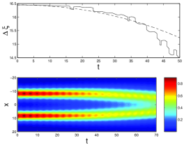
FIG. 4.: Same as in Fig. 1, but for the (attractive) interaction of in-phase breathers of the sine-Gordon equation. The breathers are initialized at a distance of $\approx 16.45$. The dashed line is the theoretical prediction of Eq. (24). The small jumps in the numerical result are an artifact of the discretization used to approximate the continuum equation. However, it can be clearly seen that the theoretical prediction follows well the full numerical evolution at least for times $t<35$, where the breathers are sufficiently well separated that the interaction has not changed their profile significantly (and for which they maintain their individual character).

Conclusions. In this short communication, we revisited the topic of solitary wave interactions for exponentially localized solutions (even though that is not absolutely necessary; however, it is typically the case) of translationally invariant, nonlinear dispersive wave equations. We showed how to systematically exploit the momentum integral to find the force exerted on one of the waves by the other and how to establish the dynamical equation of motion of the inter-soliton distance, using the mass integral and Ehrenfest’s theorem [notice that due to the structure of the energy-momentum tensor for Lorentz invariant equations, the analog of such a theorem in the latter case is given by $d/dt\int x{\cal E}dx=P$, where ${\cal E}$ is the energy density]. We demonstrated the use of the approach in a number of well-established situations, including the kink interaction in the sine-Gordon equation, the soliton interaction in the Korteweg-de Vries equation and the standing wave dynamics in the nonlinear Schrödinger equation. The method was also applied to obtain an analytical expression for the breather-breather interaction in the sine-Gordon model.

Naturally, the approach has a number of limitations: for instance it cannot be directly applied in the presence of spatially dependent potentials. Similarly, it cannot be straightforwardly implemented in cases where Ehrenfest’s theorem (or Lorentz invariance) cannot be established. A prominent such example is, for instance, the modified Korteweg-de Vries equation wherein $d/dt\int xudx=2\int u^{3}dx$, whereas the momentum is given by $\int u^{2}dx$. Certainly, it is also of interest to generalize the approach to multiple dimensions in the spirit of Ref. [13]. Finally, an alternative method to compute the interaction energy of solitary waves is through direct energy arguments: in particular, if the corresponding soliton lattice solution exists, one can compute the energy of such a solution, inside a period. The leading term will then be the energy of a single soliton, while the corrections will correspond to the soliton interaction energy. It would be interesting to compare/validate the results of such a method with those of Manton’s formalism. These topics will be deferred to future publications.

Acknowledgements. PGK acknowledges the support of NSF-DMS-0204585, NSF-CAREER and the Eppley Foundation for Research. Research at Los Alamos was supported by the U.S. Department of Energy.

REFERENCES

- [1]
- [2] M. Remoissenet, Waves called Solitons (Springer-Verlag, Berlin, 1999).
- [3] L. P. Pitaevskii and S. Stringari, Bose Einstein Condensation (Clarendon Press, Oxford, 2003); R.K. Dodd, J.C. Eilbeck, J.D. Gibbon, and H.C. Morris, Solitons and Nonlinear Wave Equations (Academic Press, London, 1982).
- [4] P.G. Drazin, Solitons (Cambridge University Press, Cambridge, 1983).
- [5] E. Infeld and G. Rowlands, Nonlinear Waves, Solitons and Chaos (Cambridge University Press, Cambridge, 2000).
- [6] Y. Kivshar and G.P. Agrawal, Optical Solitons: From Fibers to Photonic Crystals (Academic Press, San Diego, 2003).
- [7] J.M. Vogels, J.K. Chin, and W. Ketterle, Phys. Rev. Lett. 90, 030403 (2003).
- [8] P. Anninos, S. Oliveira, and R. A. Matzner, Phys. Rev. D 44, 1147 (1991).
- [9] Yu.S. Kivshar and B.A. Malomed, Rev. Mod. Phys. 61, 763 (1989).
- [10] B.A. Malomed, Progress in Optics 43, 69 (2002).
- [11] P.G. Kevrekidis, K.Ø. Rasmussen, and A.R. Bishop, Int. J. Mod. Phys. B 15, 2833 (2001); S. Flach and C.R. Willis, Phys. Rep. 295, 181 (1998).
- [12] V.I. Karpman and V.V. Solov’ev, Phys. D 3, 142 (1981); V.I. Karpman and V.V. Solov’ev, Phys. D 3, 487 (1981).
- [13] B.A. Malomed, Phys. Rev. E 58, 7928 (1998).
- [14] R. Carretero-González and K. Promislow, Phys. Rev. A 66, 033610 (2002).
- [15] C. Elphick, E. Meron, and E.A. Spiegel, SIAM J. Appl. Math. 50, 490 (1990).
- [16] B. Sandstede, Trans. Amer. Math. Soc. 350, 429 (1998).
- [17] J. M. Arnold, Phys. Rev. E 60, 979 (1999).
- [18] N.S. Manton, Nucl. Phys. B 150, 397 (1979).
- [19] J.N. Goldberg, P.S. Jang, S.Y. Park, and K.C. Wali, Phys. Rev. D 18, 542 (1978).
- [20] J.K. Perring and T.H.R. Skyrme, Nucl. Phys. 31, 550 (1962).
- [21] R. Rajaraman, Phys. Rev. D 15, 2866 (1977).
- [22] V.V. Afanasjev, B.A. Malomed, and P.L. Chu, Phys. Rev. E 56, 6020 (1997).