Stabilization mechanism for two-dimensional solitons in nonlinear parametric resonance

Abstract

We consider a simple model system supporting stable solitons in two dimensions. The system is the parametrically driven damped nonlinear Schrödinger equation, and the soliton stabilises for sufficiently strong damping. The purpose of this note is to elucidate the stabilisation mechanism; we do this by reducing the partial differential equation to a finite-dimensional dynamical system. Our conclusion is that the negative feedback loop occurs via the enslaving of the soliton’s phase, locked to the driver, to its amplitude and width.

1. When a liquid layer is subjected to vertical vibration, a one- or two-dimensional periodic pattern forms on its surface. This phenomenon has been known since the celebrated Faraday resonance experiment [1]; more recently, it was found that the vertical vibration is also capable of sustaining localised 2D states. These spatially localised, temporally oscillating structures — commonly referred to as oscillons — were observed on the surface of granular materials [2], Newtonian [3, 4] and non-Newtonian [5] fluids. Subsequently, stable oscillons were reproduced in numerical simulations within a variety of models, including the order-parameter equations [6, 4], discrete-time maps with continuous spatial coupling [7], semicontinuum [8] and hydrodynamic [9] theories. Although these simulations accounted for the formation of oscillons in several particular physical settings, they did not uncover the core of the mechanism which makes them immune from the nonlinear blow-up and dispersive broadening. The fact that stable oscillons occur in diverse physical media and in mathematical models of various nature, suggests that this mechanism is simple and general. It should operate whenever one has a balance of dispersion and nonlinearity on one hand, and of damping and phase-sensitive amplification on the other.

In order to crystallise the main ingredients of this mechanism, a simple model of nonlinear distributed system exhibiting parametric resonance was proposed recently [10]. The model comprises a two-dimensional lattice of diffusively coupled, vertically vibrated, damped pendula. In the present note we consider the associated amplitude equation whose stationary soliton solutions furnish the slowly varying amplitudes of the lattice oscillons. Understanding how these 2D stationary solitons manage to resist the nonlinear blow-up or dispersive decay in the amplitude equation will provide insights into the stabilisation of oscillons in vibrated media.

2. The amplitude equation we consider,

$$i\psi_{t}+\nabla^{2}\psi+2|\psi|^{2}\psi-\psi=h\psi^{*}-i\gamma\psi,$$ (1)

is the parametrically driven, damped nonlinear Schrödinger (NLS) equation. Here $\nabla^{2}=\partial^{2}/\partial x^{2}+\partial^{2}/\partial y^{2}.$ Apart from the pendulum lattice, eq.(1) serves as an amplitude equation for a wide range of nearly-conservative two-dimensional oscillatory systems under parametric forcing. Physically, it was used as a phenomenological model of nonlinear Faraday resonance in fluids [11, 12, 4]. Independently, it appeared in the context of optical parametric oscillators [13].

Two stationary radially-symmetric soliton solutions are given by

$$\psi_{\pm}={\cal A}_{\pm}e^{-i\theta_{\pm}}\,{\cal R}({\cal A}_{\pm}r),$$ (2)

where $r^{2}=x^{2}+y^{2}$;

$${\cal A}^{2}_{\pm}=1\pm\sqrt{h^{2}-\gamma^{2}},\quad\theta_{+}=\frac{1}{2}\arcsin\left(\frac{\gamma}{h}\right),\quad\theta_{-}=\pi-\frac{1}{2}\arcsin\left(\frac{\gamma}{h}\right),$$

and ${\cal R}(r)$ is the bell-shaped (monotonically decreasing) solution of equation

$${\cal R}_{rr}+\frac{1}{r}{\cal R}_{r}-{\cal R}+2{\cal R}^{3}=0,$$ (3)

with the boundary conditions ${\cal R}_{r}(0)={\cal R}(\infty)=0$. This solution is well documented in literature [14].

The soliton $\psi_{+}$ exists for all $h>\gamma$ while the soliton $\psi_{-}$ exists only in the wedge $\gamma<h<\sqrt{1+\gamma^{2}}$. It is pertinent to add here that when $h<\gamma$, all initial conditions are damped to zero. This follows from the rate equation

$$\partial_{t}|\psi|^{2}=2\nabla(|\psi|^{2}\nabla\chi)+2|\psi|^{2}(h\sin 2\chi-\gamma),$$ (4)

where $\chi$ is the phase of the field $\psi$: $\psi=|\psi|e^{-i\chi}$. Defining

$$N=\int|\psi|^{2}d{\bf x},$$

eq.(4) implies

$$\partial_{t}{N}\leq 2(h-\gamma)N,$$

whence $N(t)\to 0$ as $t\to\infty$. We should also mention here that on the other side of the wedge, i.e. for $h>\sqrt{1+\gamma^{2}}$, all solutions with $\psi\to 0$ as $|x|\to\infty$ are unstable against nonlocalised (continuous spectrum) perturbations [15].

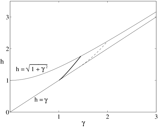
Figure 1: Stability diagram for the two-dimensional soliton ($\psi_{+}$). No stationary localised solutions exist below the straight line $h=\gamma$, while above the ‘parabola’ $h=\sqrt{1+\gamma^{2}}$ all localised solutions are unstable to radiation waves. The region of stability of the soliton lies between the straight line and ‘parabola’, to the right of the thick solid curve. The dashed curve gives the variational approximation to the stability boundary: $h=(1+\gamma^{4}/4)^{1/2}$, $\gamma\geq\sqrt{2}$.

In the absence of the damping and driving, i.e. when $h=\gamma=0$, all localised initial conditions in the two-dimensional NLS equation are known to either disperse or blow-up in finite time [14, 16]. Recently it was shown, however, that while the soliton $\psi_{-}$ remains unstable for all $h$ and $\gamma$, the soliton $\psi_{+}$ stabilises for sufficiently strong damping and driving [10]. (The smallest value of $\gamma$ for which this soliton can be stable, is 1.006.) The corresponding stability chart is shown in Fig.1. Our purpose is to explain, in qualitative terms, the stabilization mechanism that is at work here.

3. To this end, we use the variational approach. Equation (1) is derivable from the stationary action principle with the Lagrangian

$${\cal L}=e^{2\gamma t}\,{\rm Re\/}\int(i\psi_{t}\psi^{*}-|\nabla\psi|^{2}-|\psi|^{2}+|\psi|^{4}-h\psi^{2})d{\bf x}.$$ (5)

Choosing a bell-shaped trial function [17]

$$\psi=\sqrt{A}e^{-i\theta-(B+i\sigma)r^{2}},$$

with $A,B,\theta,$ and $\sigma$ real functions of $t$, the Lagrangian (5) reduces to

$${\cal L}=e^{2\gamma t}\,\frac{A}{B}\left[{\dot{\theta}}-1+\frac{\dot{\sigma}}{2B}-\frac{2B}{\cos^{2}\phi}+\frac{A}{2}-h\cos(\phi+2\theta)\cos\phi\right],$$ (6)

with $\tan\phi=\sigma/B$. The corresponding Euler-Lagrange equations are

$${\dot{A}} = 8\sigma A-2\gamma A+4hA\sin(\phi+2\theta)\cos\phi-2hA\sin[2(\phi+\theta)]\cos^{2}\phi,$$ (7)

$${\dot{B}} = 8\sigma B+2hB\sin(\phi+2\theta)\cos\phi-2hB\sin[2(\phi+\theta)]\cos^{2}\phi,$$ (8)

$${\dot{\theta}} = 1+4B-\frac{3}{2}A+2h\cos(\phi+2\theta)\cos\phi-h\cos[2(\phi+\theta)]\cos^{2}\phi,$$ (9)

$${\dot{\sigma}} = 4\sigma^{2}-4B^{2}+AB-2hB\cos(\phi+2\theta)\cos\phi$$ (10)

$$+2hB\cos[2(\phi+\theta)]\cos^{2}\phi.$$

The four-dimensional dynamical system defined by (7)-(10) has two fixed points representing the two stationary solitons:

$$A_{\pm}=2\left(1\pm\sqrt{h^{2}-\gamma^{2}}\right),\quad B_{\pm}=\frac{A_{\pm}}{4},$$

$$\theta_{+}=\frac{1}{2}\arcsin{\frac{\gamma}{h}},\quad\theta_{-}=\pi-\frac{1}{2}\arcsin{\frac{\gamma}{h}},\quad\sigma_{\pm}=0.$$

Consistently with the stability properties of the solitons in the full PDE (1), the fixed point $(A_{-},\,B_{-})$ is unstable for all $h$ and $\gamma$ whereas the point $(A_{+},\,B_{+})$ is unstable for small $\gamma$ but stabilises for larger dampings. (More precisely, this stationary point is stable in the region described by $h>\sqrt{1+\gamma^{4}/4}$, with $\gamma\geq\sqrt{2}$ — see Fig.1.) Therefore, the four-mode approximation captures the essentials of the infinite-dimensional dynamics in the localised-waveform sector. We will now establish two constraints reducing the number of independent degrees of freedom to two; these constraints will eventually provide the key to the stability mechanism.

4. The two-dimensional reduction arises in the overdamped limit, i.e. for large $\gamma$. In this limit, the dynamics should occur on a slow time-scale; hence we introduce the “slow” time $T=t/\gamma$. We can also expand the solution in powers of the small parameter $\gamma^{-1}$:

$$A = A_{0}+\frac{1}{\gamma}A_{1}+...,\quad B=B_{0}+\frac{1}{\gamma}B_{1}+...,$$

$$\theta = \frac{\pi}{4}+\frac{1}{\gamma}\theta_{1}+...,\quad\sigma=\frac{1}{\gamma}\sigma_{1}+....$$

Letting $h=\gamma+c/(2\gamma)$ with $0\leq c\leq 1$, we make sure that $h$ lies in the region of interest: $\gamma<h<\sqrt{1+\gamma^{2}}$. Substituting in (7)-(10) and matching coefficients of like powers of $\gamma^{-1}$, yields a two-dimensional system

$$\frac{dA_{0}}{dT} = A_{0}[c+8\sigma_{1}-4\theta_{1}^{2}+2(\sigma_{1}/B_{0})^{2}],$$ (11)

$$\frac{dB_{0}}{dT} = 8\sigma_{1}B_{0}+4\sigma_{1}\theta_{1}+4(\sigma_{1}^{2}/B_{0}),$$ (12)

where

$$\theta_{1} = \frac{1}{2}+2B_{0}-\frac{3}{4}A_{0},$$ (13)

$$\sigma_{1} = \frac{1}{2}A_{0}B_{0}-2B_{0}^{2}.$$ (14)

Like their parent system, eqs.(11)-(12) have two stationary points in the first quadrant of the $(A_{0},B_{0})$-plane,

$$B_{0}^{\pm}=\frac{1\pm\sqrt{c}}{2},\quad A_{0}^{\pm}=4B_{0}^{\pm},$$

with $\theta_{1}^{\pm}=\mp\sqrt{c}/2$ and $\sigma_{1}^{\pm}=0$. (Since the $A_{0}$- and $B_{0}$-axis are invariant manifolds, we can restrict our attention to the first quadrant only. In particular, fixed points with $A_{0}<0$ or $B_{0}<0$ can have no effect on the dynamics in the first quadrant.) Like in system (7)-(10) with large $\gamma$, the fixed point $(A_{0}^{+},\,B_{0}^{+})$ is stable (a stable focus) and the other fixed point, $(A_{0}^{-},\,B_{0}^{-})$, is unstable (a saddle). The sink at the origin is another attractor in the system, competing with the “soliton” $(A_{0}^{+},B_{0}^{+})$. The corresponding basins of attraction are separated by the stable manifold of the saddle (see Fig.2). As $t\to-\infty$, the top part of the separatrix (along with many other trajectories) satisfies $A_{0},B_{0}\to\infty$ with $A_{0}\propto B_{0}^{7/2}$.

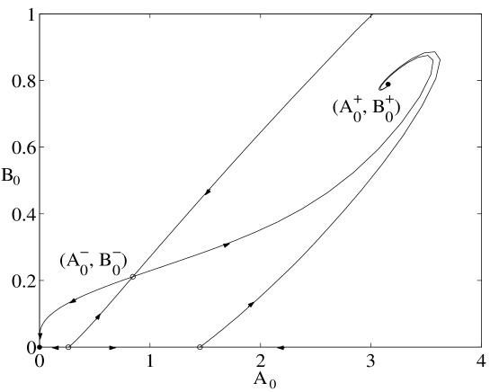
Figure 2: Phase portrait of the vector field (11)-(12). (In this plot, $c=1/3$.) The stable manifold of the saddle $(A_{0}^{-},B_{0}^{-})$ separates the plane into the basins of attraction of the node at the origin and focus at $(A_{0}^{+},B_{0}^{+})$.

The most important conclusion of the finite-dimensional analysis is summarised by eqs.(13)-(14): two of the four modes are enslaved by the other two. It is fitting to note here that the division into the “masters” and “slaves” is somewhat arbitrary; although in (11)-(14) the amplitude and width appear as “master” modes and the two components of the phase as “slaves”, the reduction can be easily reformulated in such a way that, for example, $\theta$ and $\sigma$ are the masters and $A$ and $B$ are the slaves. All one needs to do is express $A_{0}$ and $B_{0}$ through $\theta_{1}$ and $\sigma_{1}$ from (13) and (14), and substitute into (11) and (12).

5. In order to explain the stability mechanism, we turn to equation (4) governing the density of the soliton’s elementary constituents, $|\psi|^{2}$. [If eq.(1) is used to model Faraday resonance in granular media, $\int|\psi|^{2}$ dx has the meaning of the total number of particles captured in the oscillon.] The first term on the right-hand side of (4) does not affect the total number of the constituents. All it does is rearranges the constituents across the oscillon. The second term, on the contrary, does give rise to the creation and annihilation of particles. Since this term is proportional to $|\psi|^{2}$, the creation and annihilation occur mainly in the core of the oscillon, where $|\psi|^{2}$ is not small. In the core we have $r\sim 0$ and so the creation and annihilation is controlled by $\theta$, the uniform component of the phase

$$\chi=\theta+\sigma r^{2}.$$ (15)

The nonuniform part of the phase, $\sigma r^{2}$, is small in the core and plays a secondary role in this process. Instead, the significance of the quantity $\sigma$ is in that it controls the flux of the constituents between the core and the periphery of the soliton — see the $\nabla\chi$-term in the r.h.s. of (4).

If we perturb the stationary point $\psi_{+}$ in the 4-dimensional phase space of (7)-(10), the variables $\theta$ and $\sigma$ will zap, within a very short time $\Delta t\sim\frac{1}{\gamma}$, onto the 2-dimensional subspace defined by the constraints (13)-(14). After this short transient, the evolution of $\theta$ and $\sigma$ will be immediately following that of the soliton’s amplitude $\sqrt{A}$ and width $1/\sqrt{B}$. Since the phase $\chi$ is coupled to the driver, this provides a negative feedback: perturbations in $A$ and $B$ produce only such changes in the two parts of the phase that the new values of $\chi(r)$ stimulate the recovery of the stationary values of $A$ and $B$. (The flat phase $\theta$ works to restore the number of constituents while the chirp $\sigma$ rearranges them across the soliton.)

This can be illustrated by considering $\psi$ as the envelope of an oscillon on the surface of a granular layer, e.g. a layer of tiny brass beads — as in the original experiment [2]. Imagine that we increase the amplitude $\sqrt{A}$ of the oscillon (for example, by dropping several beads on its top): $\delta A_{0}(0)>0$. Assume, for simplicity, that we do this without changing the oscillon’s width: $\delta B_{0}(0)=0$. From eqs.(13),(14) it follows then that $\delta\theta_{1}(0)<0$. Since the angle $2\chi=2(\pi/4+\gamma^{-1}\theta_{1}^{+})$ is acute for the stationary point $(A_{0}^{+},B_{0}^{+})$ (remember, $\theta_{1}^{+}<0$ and $\sigma^{+}_{1}=0$), the decrease in $\theta$ produces a decrease in $\sin 2\chi$. (Here $\chi$ is given by eq.(15).) As a result, the second term in the right-hand side of eq.(4) becomes negative which triggers the annihilation of elementary constituents. (In the experimental situation this simply means that the oscillon starts “leaking” beads to the surrounding medium.) The annihilation continues until the original, stationary, value of $\chi$ (and hence, the original value of $A=A_{+}$) is recovered.

Why does this mechanism not work in the case of the unstable fixed point, $(A_{0}^{-},B_{0}^{-})$? The difference is that in that case, $\theta_{1}^{-}>0$ and so $2\chi=2(\pi/4+\gamma^{-1}\theta_{1}^{-})$ is an obtuse angle. Therefore adding particles at the initial moment of time and the resulting decrease of the phase $\chi$ give rise to an increase of $\sin 2\chi$. The second term in the right-hand side of (4) becomes positive and this triggers a further creation of elementary constituents (that is, more brass beads will be pulled into the oscillon from the surrounding layer.) Hence this time the feedback is positive which makes the stabilisation impossible.

Finally, why is the large damping essential for stability? For small $\gamma$ the coupling of $\theta$ and $\sigma$ to $A$ and $B$ is via differential rather than algebraic equations. This time, the dynamics of $\theta$ and $\sigma$ is inertial and so the evolution of the phase may not catch up with that of the amplitude and width. The feedback loop breaks down and the soliton destabilises.

In conclusion, the stabilisation mechanism comprises two main ingredients: (a) the enslaving of two essential degrees of freedom (e.g. the flat and quadratic components of the phase) by another two (amplitude and effective width of the soliton); and (b) locking of the phase (and thereby of the amplitude and width) to the parametric driver.

Acknowledgment. This project was supported by grants from the URC of the University of Cape Town, and National Research Foundation of South Africa.

References

- [1] H.W. Müller, R. Friedrich, D. Papathanassiou. Theoretical and Experimental Investigation of the Faraday Instability. In: F. Busse and S.C. Müller (Eds.), Evolution of Spontaneous Structures in Dissipative Continuous Systems, Lecture Notes in Physics, vol.55, Springer, New York, 1998, pp.231-265
- [2] P.B. Umbanhowar, F. Melo, and H.L. Swinney, Nature 382, 793 (1996)
- [3] O. Lioubashevski, H. Arbell, and J. Fineberg, Phys. Rev. Lett. 76, 3959 (1996); H. Arbell and J. Fineberg, ibid. 85, 756 (2000)
- [4] D. Astruc and S. Fauve. Parametrically Amplified 2-Dimensional Solitary Waves. In: A.C. King and Y.D. Shikhmurzaev (Eds.), IUTAM Symposium on Free Surface Flows. Fluid Mechanics and Its Applications, vol. 62, Kluwer, Boston, 2001, pp.39-46
- [5] O. Lioubashevski, Y. Hamiel, A. Agnon, Z. Reches, and J. Fineberg, Phys. Rev. Lett. 83, 3190 (1999)
- [6] L.S. Tsimring and I.S. Aranson, Phys. Rev. Lett. 79, 213 (1997); H. Sakaguchi, H.R. Brand, Europhys. Lett. 38, 341 (1997); Physica D 117, 95 (1998); C. Crawford, H. Riecke, Physica D 129, 83 (1999)
- [7] E. Cerda, F. Melo, and S. Rica, Phys. Rev. Lett. 79, 4570 (1997); S.C. Venkataramani and E. Ott, Phys. Rev. Lett. 80, 3495 (1998); S.-O. Jeong, T.-W. Ko, H.-T. Moon, Physica D 164, 71 (2002)
- [8] D. Rothman, Phys. Rev. E 57, 1239 (1998)
- [9] J. Eggers and H. Riecke, Phys. Rev. E 59, 4476 (1999)
- [10] I.V. Barashenkov, N.V. Alexeeva, and E.V. Zemlyanaya, Phys. Rev. Lett. 89, 104101 (2002)
- [11] S.V. Kiyashko, L.N. Korzinov, M.I. Rabinovich, and L.S. Tsimring, Phys. Rev. E 54, 5037 (1996)
- [12] W. Zhang and J. Viñals, Phys. Rev. Lett. 74, 690 (1995)
- [13] V.J. Sánchez-Morcillo, I. Pérez-Arjona, F. Silva, G.J. de Valcárel, and E. Roldán, Opt. Lett. 25, 957 (2000); I. Pérez-Arjona, E. Roldán, and G.J. de Valcárcel, arXiv:quant-ph/0405148
- [14] See e.g. K. Rypdal, J.J. Rasmussen and K. Thomsen, Physica D 16, 339 (1985) and references therein.
- [15] I.V. Barashenkov, M.M. Bogdan and V.I. Korobov, Europhys. Lett. 15, 113 (1991)
- [16] E.A. Kuznetsov and S.K. Turitsyn, Phys. Lett. 112A, 273 (1985); V.M. Malkin and E.G. Shapiro, Physica D 53, 25 (1991).
- [17] This ansatz is frequently employed in studies of blowup phenomena, see e.g. V.E. Zakharov and E.A. Kuznetsov, ZhETF 91, 1310 (1986) [Sov. Phys. JETP 64, 773 (1986)]