Nodal two-dimensional solitons in nonlinear parametric resonance

Abstract

The parametrically driven damped nonlinear Schrödinger equation serves as an amplitude equation for a variety of resonantly forced oscillatory systems on the plane. In this note, we consider its nodal soliton solutions. We show that although the nodal solitons are stable against radially-symmetric perturbations for sufficiently large damping coefficients, they are always unstable to azimuthal perturbations. The corresponding break-up scenarios are studied using direct numerical simulations. Typically, the nodal solutions break into symmetric “necklaces” of stable nodeless solitons.

1. Two-dimensional localised oscillating structures, commonly referred to as oscillons, have been detected in experiments on vertically vibrated layers of granular material [1], Newtonian fluids and suspensions [2, 3]. Numerical simulations established the existence of stable oscillons in a variety of pattern-forming systems, including the Swift-Hohenberg and Ginsburg-Landau equations, period-doubling maps with continuous spatial coupling, semicontinuum theories and hydrodynamic models [3, 4]. These simulations provided a great deal of insight into the phenomenology of the oscillons; however, the mechanism by which they acquire or loose their stability remained poorly understood.

In order to elucidate this mechanism, a simple model of a parametrically forced oscillatory medium was proposed recently [5]. The model comprises a two-dimensional lattice of diffusively coupled, vertically vibrated pendula. When driven at the frequency close to their double natural frequency, the pendula execute almost synchronous librations whose slowly varying amplitude satisfies the 2D parametrically driven, damped nonlinear Schrödinger (NLS) equation. The NLS equation was shown to support radially-symmetric, bell-shaped (i.e. nodeless) solitons which turned out to be stable for sufficiently large values of the damping coefficient. These stationary solitons of the amplitude equation correspond to the spatio-temporal envelopes of the oscillons in the original lattice system. By reducing the NLS to a finite-dimensional system in the vicinity of the soliton, its stabilisation mechanism (and hence, the oscillon’s stabilisation mechanism) was clarified [5].

In the present note we consider a more general class of radially-symmetric solitons of the parametrically driven, damped NLS on the plane, namely solitons with nodes. We will demonstrate that these solitons are unstable against azimuthal modes, and analyse the evolution of this instability.

2. The parametrically driven, damped NLS equation has the form:

$$i\psi_{t}+\nabla^{2}\psi+2|\psi|^{2}\psi-\psi=h\psi^{*}-i\gamma\psi.$$ (1)

Here $\nabla^{2}=\partial^{2}/\partial x^{2}+\partial^{2}/\partial y^{2}.$ Eq.(1) serves as an amplitude equation for a wide range of nearly-conservative two-dimensional oscillatory systems under parametric forcing. This equation was also used as a phenomenological model of nonlinear Faraday resonance in water [3]. The coefficient $h>0$ plays the role of the driver’s strength and $\gamma>0$ is the damping coefficient.

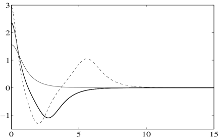
Figure 1: Solutions of eq.(3): ${\cal R}_{0}(r)$ (thin continuous line), ${\cal R}_{1}(r)$ (thick line), ${\cal R}_{2}(r)$ (dashed).

We start with the discussion of its nodeless solitons and their stability. The exact (though not explicit) stationary radially-symmetric solution is given by

$$\psi_{0}={\cal A}e^{-i\theta}\,{\cal R}_{0}({\cal A}r),$$ (2)

where $r^{2}=x^{2}+y^{2}$,

$${\cal A}^{2}=1+\sqrt{h^{2}-\gamma^{2}},\quad\theta=\frac{1}{2}\arcsin\left(\frac{\gamma}{h}\right),$$

and ${\cal R}_{0}(r)$ is the bell-shaped nodeless solution of the equation

$${\cal R}_{rr}+\frac{1}{r}{\cal R}-{\cal R}+2{\cal R}^{3}=0$$ (3)

with the boundary conditions ${\cal R}_{r}(0)={\cal R}(\infty)=0$. (Below we simply write ${\cal R}$ for ${\cal R}_{0}$.) Solutions of eq.(3) are well documented in literature [6]; see Fig.1.

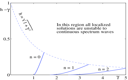
Figure 2: Stability diagram for two-dimensional solitons. The $(\gamma,h-\gamma)$-plane is used for visual clarity. No localised or periodic attractors exist for $h<\gamma$ (below the horisontal axis). The region of stability of the soliton $\psi_{0}$ lies to the right of the solid curve marked “$n=0$”. Also shown are the regions of stability of the solitons $\psi_{1}$ and $\psi_{2}$ with respect to the radially-symmetric perturbations. (These lie to the right of the corresponding curves in the figure.)

3. To examine the stability of the solution (2) with nonzero $h$ and $\gamma$, we linearise eq.(1) in the small perturbation

$$\delta\psi({\bf x},t)=e^{(\mu-\Gamma){\tilde{t}}-i\theta_{\pm}}[u({\tilde{\bf x}})+iv({\tilde{\bf x}})],$$

where ${\tilde{\bf x}}={\cal A}{\bf x}$, ${\tilde{t}}={\cal A}^{2}t$. This yields an eigenvalue problem

$$L_{1}u=-(\mu+\Gamma)v,\quad(L_{0}-\epsilon)v=(\mu-\Gamma)u,$$ (4)

where $\Gamma=\gamma/{\cal A}^{2}$ and the operators

$$L_{0}\equiv-{\tilde{\nabla}}^{2}+1-2{\cal R}^{2}({\tilde{r}}),\quad L_{1}\equiv L_{0}-4{\cal R}^{2}({\tilde{r}}),$$ (5)

with ${\tilde{\nabla}}^{2}=\partial^{2}/\partial{\tilde{x}}^{2}+\partial^{2}/\partial{\tilde{y}}^{2}$. (We are dropping the tildas below.) For further convenience, we introduce the positive quantity $\epsilon=2\sqrt{h^{2}-\gamma^{2}}/{\cal A}^{2}$. Fixing $\epsilon$ defines a curve on the $(\gamma,h)$-plane:

$$h=\sqrt{\epsilon^{2}/(2-\epsilon)^{2}+\gamma^{2}}.$$ (6)

Introducing

$$\lambda^{2}=\mu^{2}-\Gamma^{2}$$ (7)

and performing the transformation [9]

$$v({\bf x})\to(\mu+\Gamma)\lambda^{-1}v({\bf x}),$$

reduces eq.(4) to a one-parameter eigenvalue problem:

$$(L_{0}-\epsilon)v=\lambda u,\quad L_{1}u=-\lambda v.$$ (8)

We first consider the stability with respect to radially symmetric perturbations $u=u(r),\,v=v(r)$. In this case the operators (5) become

$$L_{0}=-\frac{d^{2}}{dr^{2}}-\frac{1}{r}\frac{d}{dr}+1-2{\cal R}^{2}(r),\quad L_{1}=L_{0}-4{\cal R}^{2}(r).$$ (9)

In the absence of the damping and driving, all localised initial conditions in the unperturbed 2D NLS equation are known to either disperse or blow-up in finite time [6, 7, 8]. It turned out, however, that the soliton $\psi_{0}$ stabilises as the damping $\gamma$ is increased above a certain value [5]. The stability condition is $\gamma\geq\gamma_{c}$, where

$$\gamma_{c}=\gamma_{c}(\epsilon)\equiv\frac{2}{2-\epsilon}\cdot\frac{{\rm Re\/}\lambda(\epsilon)\,{\rm Im\/}\lambda(\epsilon)}{\sqrt{({\rm Im\/}\lambda)^{2}-({\rm Re\/}\lambda)^{2}}}.$$ (10)

We obtained $\lambda(\epsilon)$ by solving the eigenvalue problem (8) directly. Expressing $\epsilon$ via $\gamma_{c}$ from (10) and feeding into (6), we get the stability boundary on the $(\gamma,h)$-plane (Fig.2).

4. To study the stability to asymmetric perturbations we factorise, in (8),

$$u({\bf x})={\tilde{u}}(r)e^{im\varphi},\quad v({\bf x})={\tilde{v}}(r)e^{im\varphi},$$

where $\tan\varphi=y/x$ and $m$ is an integer. The functions ${\tilde{u}}(r)$ and ${\tilde{v}}(r)$ satisfy the eigenproblem (8) where the operators (9) should be replaced by

$$L_{0}^{(m)}\equiv L_{0}+{m^{2}}/{r^{2}},\quad L_{1}^{(m)}\equiv L_{1}+{m^{2}}/{r^{2}},$$ (11)

respectively. This modified eigenvalue problem can be analysed in a similar way to eqs.(8). It is not difficult to demonstrate that all discrete eigenvalues of (8) (if any exist) have to be pure imaginary in this case, and hence the azimuthal perturbations do not lead to any instabilities of the solution in question [5].

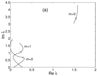
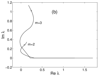
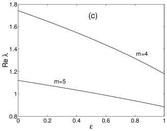
Figure 3: The discrete eigenvalues of the linearised operator (8) for the one-node soliton, $\psi_{1}$. Panels (a) and (b) show the complex eigenvalues, $\mbox{Im}\,\lambda$ vs $\mbox{Re}\,\lambda$. Arrows indicate the direction of increase of $\epsilon$. Panel (c) shows the real eigenvalues, as functions of $\epsilon$.

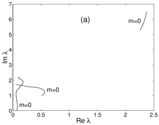
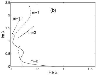
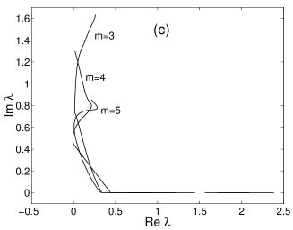
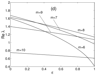
Figure 4: The discrete eigenvalues of the linearised operator (8) for the two-node soliton, $\psi_{2}$. Panels (a),(b), and (c) show the complex eigenvalues, $\mbox{Im}\,\lambda$ vs $\mbox{Re}\,\lambda$. Panel (d) shows the real eigenvalues, as functions of $\epsilon$.

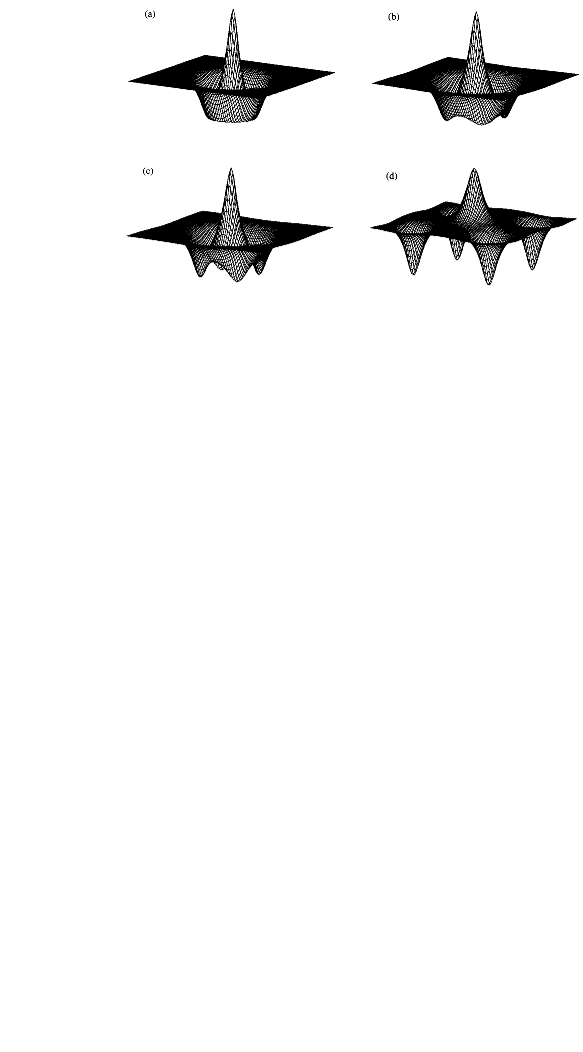
Figure 5: Evolution of the azimuthal instability of the one-node soliton. (a): the initial condition, soliton $\psi_{1}$ ; (b) and (c): dissociation of the ring-like “valley” into 4 nodeless solitons; (d): divergence of the fragments. Here $\gamma=3.5$ and $h=3.6$; shown is $\mbox{Re}\,\psi$. Note the change of the vertical scale in (d).

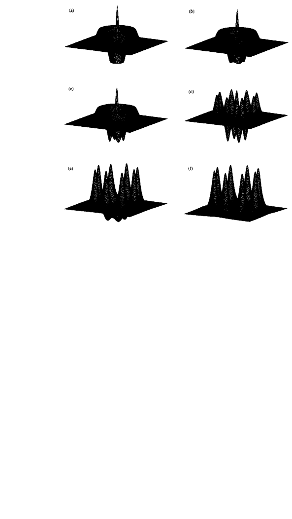
Figure 6: The evolution of the azimuthal instability of the two-node soliton $\psi_{2}$. (a): the initial condition; (b)-(c): the rapid dissociation of the “valley” into 4 nodeless solitons; (c)-(d): a slower decay of the “ridge” into 8 solitons $\psi_{0}$; (e)-(f): the annihilation of the internal ring and the central soliton, and the repulsion of the persisting 8 solitons. Here $\gamma=4.5$ and $h=4.53$; shown is $\mbox{Re}\,\psi$. Note the change of the vertical scale in (e)-(f) w.r.t. that in (a)-(d).

5. Besides the nodeless solution ${\cal R}_{0}(r)$, the “master” equation (3) has solutions ${\cal R}_{n}(r)$ with $n$ nodes, $n\geq 1$. (See Fig.1). These give rise to a sequence of nodal solutions $\psi_{n}$ of the damped-driven NLS (1), defined by eq.(2) with ${\cal R}_{0}\to{\cal R}_{n}$. To examine the stability of the $\psi_{n}$, we solved the eigenvalue problem (8) numerically, with operators $L_{0,1}^{(m)}$ as in (11). The radial stability properties of the nodal solitons turned out to be similar to those of the nodeless soliton $\psi_{0}$. Namely, the $\psi_{n}$ solutions are stable against radially-symmetric perturbations for sufficiently large $\gamma$. The corresponding stability regions for $\psi_{1}$ and $\psi_{2}$ are depicted in Fig.(2). However, the azimuthal stability properties of the nodal solitons have turned out to be quite different.

Both $\psi_{1}$ and $\psi_{2}$ solutions do have eigenvalues $\lambda$ with nonzero real parts for orbital numbers $m\geq 1$. (See Fig.3 and 4.) Having found eigenvalues $\lambda$ for each $\epsilon$, one still has to identify those giving rise to the largest growth rates

$$\nu=\mbox{Re}\,\mu-\Gamma$$ (12)

for each pair $(\epsilon,\gamma)$ [or, equivalently, for each $(h,\gamma)$]. In (12), $\mu$ is reconstructed using eq.(7). The selection of real eigenvalues is straightforward; in this case we have the following two simple rules:
$\bullet$ If, for some $\epsilon$, there are eigenvalues $\lambda_{1}>0$, $\lambda_{2}>0$ such that $\lambda_{1}>\lambda_{2}$, then $\nu_{1}>\nu_{2}$ for this $\epsilon$ and all $\gamma$. That is, of all real eigenvalues $\lambda$ one has to consider only the largest one.
$\bullet$ If, for some $\epsilon$, there is a real eigenvalue $\lambda_{1}>0$ and a complex eigenvalue $\lambda_{2}$, with $\mbox{Re}\,\lambda_{2}>0$ and $\lambda_{1}>\mbox{Re}\,\lambda_{2}$, then $\nu_{1}>\nu_{2}$ for this $\epsilon$ and all $\gamma$. That is, one can ignore all complex eigenvalues with real parts smaller than a real eigenvalue — if there is one.

The comparison of two complex eigenvalues is not so straightforward. In particular, the fact that $\mbox{Re}\,\lambda_{1}>\mbox{Re}\,\lambda_{2}$ does not necessarily imply that $\nu_{1}>\nu_{2}$. Which of the two growth rates, $\nu_{1}$ or $\nu_{2}$, is larger will depend on the imaginary parts of $\lambda$, as well as on $\gamma$.

In figures 3 and 4, we illustrate the real and imaginary parts of the eigenvalues, arising for different $m$, for the solitons $\psi_{1}$ and $\psi_{2}$. The soliton $\psi_{1}$ has discrete eigenvalues $\lambda$ associated with orbital numbers $m=0,1,...,5$ and the soliton $\psi_{2}$ with $m=0,1,...,10$.

m	$\nu$	Re$\lambda$	Im$\lambda$		m	$\nu$	Re$\lambda$	Im$\lambda$
0	-0.1620	1.5797	4.2181		0	-0.3361	2.3531	6.1585
0	-1.4827	0.0609	1.8743		0	-0.5877	0.1819	1.7847
					0	-0.4168	0.3093	1.5572
1	-0.8255	0.2272	1.6198		1	-0.8089	0.3818	2.1021
1	2.79e-6	0.0033	0.0000		1	-0.4891	0.1111	1.6352
					1	1.07e-5	0.0079	0.0000
2	-0.3012	0.2213	1.0602		2	-0.3497	0.3737	1.4597
					2	-0.0328	0.2602	0.5128
3	0.0872	0.5821	0.0000		3	0.5406	1.8686	0.0000
4	0.3689	1.2399	0.0000		4	0.5286	1.8462	0.0000
5	0.2057	0.9076	0.0000		5	0.0263	0.3958	0.0000
					6	0.1611	0.9898	0.0000
					7	0.2490	1.2392	0.0000
					8	0.2783	1.3133	0.0000
					9	0.2288	1.1861	0.0000
					10	0.0720	0.6567	0.0000

Table 1: Eigenvalues $\lambda$ and corresponding growth rates $\nu$ for the solitons $\psi_{1}$ (left panel) and $\psi_{2}$ (right panel). We included only the eigenvalues which can, potentially, give rise to the largest growth rate in each “symmetry class” $m$. Some other eigenvalues have been filtered out using the above selection rules.

In order to compare the conclusions based on the linearised analysis with direct numerical simulations of the unstable solitons $\psi_{1}$ and $\psi_{2}$, we fix some $h$ and $\gamma$ and identify the eigenvalue with the maximum growth rate in each case. In the case of the soliton $\psi_{1}$, we choose $\gamma=3.5$ and $h=3.6$; the corresponding $\epsilon=0.9146$. The real and imaginary parts of $\lambda$ for each $m$ as well as the resulting growth rates $\nu$ are given in Table 1 (left panel). The eigenvalue with the largest ${\rm Re}\lambda$ is associated with $m=0$; however, for the given $\epsilon$ and $\gamma$ the resulting $\nu<0$. (This is because we have chosen a point in the “radially stable” part of the $(\gamma,h)$-plane, to the right of the “$n=1$” curve in Fig.2.) On the contrary, the growth rates corresponding to the real eigenvalues associated with $m=3,4,5$ are positive for all $\gamma$. The maximum growth rate is associated with $m=4$. The corresponding eigenfunctions $u(r)$ and $v(r)$ have a single maximum near the position of the minimum of the function ${\cal R}_{1}(r)$; that is, the perturbation is concentrated near the circular “valley” in the relief of $\psi(x,y)|^{2}$. This observation suggests that for $\gamma=3.4$ and $h=3.5$, the soliton $\psi_{1}$ should break into a symmetric pattern of 5 solitons $\psi_{0}$: one at the origin and four around it.

Next, in the case of the soliton $\psi_{2}$ we fix $\gamma=4.5$ and $h=4.53$; this gives $\epsilon=0.6846$. The corresponding eigenvalues, for each $m$, are presented in Table 1 (right panel). Again, the eigenvalue with the largest $\mbox{Re}\lambda$ is the one for $m=0$ but the resulting $\nu$ is negative. The largest growth rates ($\nu_{3}=0.54$ and $\nu_{4}=0.53$, respectively) are those pertaining to $m=3$ and $m=4$. The corresponding eigenfunctions have their maxima near the position of the minimum of the function ${\cal R}_{2}(r)$. Therefore, the circular “valley” of the soliton $\psi_{2}$ is expected to break into three or four nodeless solitons $\psi_{0}$. (Since $\nu_{3}$ is so close to $\nu_{4}$, the actual number of resulting solitons — three or four — will be very sensitive to the choice of the initial perturbation.) Next, eigenfunctions pertaining to $m=5,6,...10$ have their maxima near the second, lateral, maximum of the function ${\cal R}_{2}(r)$. The largest growth rate in this group of eigenvalues arises for $m=8$. Hence, the circular “ridge” of the soliton $\psi_{2}$ should break into 8 nodeless solitons, with this process taking longer than the bunching of the “valley” into the “internal ring” of solitons.

The direct numerical simulations corroborate the above scenarios. The $\psi_{1}$ soliton with $\gamma=3.5$ and $h=3.6$ splits into a constellation of 5 nodeless solitons: one at the origin and four solitons of opposite polarity at the vertices of the square centered at the origin. The emerging nodeless solitons are stable but repelling each other, see Fig.5. Hence, no stationary nonsymmetric configurations are possible; the peripheral solitons escape to infinity. The $\psi_{2}$ soliton with $\gamma=4.5$ and $h=4.53$ has a more complicated evolution. As predicted by the linear stability analysis, it dissociates into 13 nodeless solitons: one at the origin, four solitons of opposite polarity forming a square around it and eight more solitons (of the same polarity as the one at the origin) forming an outer ring. (The fact that the inner ring consists of four and not three solitons, is due to the square symmetry of our domain of integration which favours perturbations with $m=4$ over those with $m=3$.) In the subsequent evolution the central soliton and the nearest four annihilate and only the eight outer solitons persist. They repel each other and eventually escape to infinity, see Fig.6.

In conclusion, our analysis suggests the interpretation of the nodal solutions as degenerate, unstable coaxial complexes of the nodeless solitons $\psi_{0}$.

Acknowledgements. This project was supported by the NRF of South Africa under grant 2053723. The work of E.Z. was supported by an RFBR grant 03-01-00657.

References

- [1] P.B. Umbanhowar, F. Melo, and H.L. Swinney, Nature 382, 793 (1996)
- [2] O. Lioubashevski et al, Phys. Rev. Lett. 83, 3190 (1999); H. Arbell and J. Fineberg, ibid. 85, 756 (2000)
- [3] D. Astruc and S. Fauve, in: Fluid Mechanics and Its Applications, vol.62, p. 39-46 (Kluwer, 2001)
- [4] L.S. Tsimring and I.S. Aranson, Phys. Rev. Lett. 79, 213 (1997); E. Cerda, F. Melo, and S. Rica, ibid. 79, 4570 (1997); S.C. Venkataramani and E. Ott, ibid. 80, 3495 (1998); D. Rothman, Phys. Rev. E 57, 1239 (1998); J. Eggers and H. Riecke, ibid. 59, 4476 (1999); C. Crawford, H. Riecke, Physica D 129, 83 (1999); H. Sakaguchi, H.R. Brand, Europhys. Lett. 38, 341 (1997); Physica D 117, 95 (1998)
- [5] I.V. Barashenkov, N.V. Alexeeva, and E.V. Zemlyanaya, Phys. Rev. Lett. 89, 104101 (2002)
- [6] See e.g. K. Rypdal, J.J. Rasmussen and K. Thomsen, Physica D 16, 339 (1985) and references therein.
- [7] E.A. Kuznetsov and S.K. Turitsyn, Phys. Lett. 112A, 273 (1985); V.M. Malkin and E.G. Shapiro, Physica D 53, 25 (1991)
- [8] For a recent review and references on the blowup in 2D and 3D NLS equations, see e.g. L. Berge, Phys. Rep. 303, 259 (1998); G. Fibich and G. Papanicolaou, SIAM J. Appl. Math. 60, 183 (1999)
- [9] I.V. Barashenkov, M.M. Bogdan and V.I. Korobov, Europhys. Lett. 15, 113 (1991)