Gap solitons in a model of a hollow optical fiber

Abstract

We introduce a models for two coupled waves propagating in a hollow-core fiber: a linear dispersionless core mode, and a dispersive nonlinear quasi-surface one. The linear coupling between them may open a bandgap, through the mechanism of the avoidance of crossing between dispersion curves. The third-order dispersion of the quasi-surface mode is necessary for the existence of the gap. Numerical investigation reveals that the entire bandgap is filled with solitons, and they all are stable in direct simulations. The gap-soliton (GS) family is extended to include pulses moving relative to the given reference frame, up to limit values of the corresponding boost $\delta$, beyond which the solitons do not exists. The limit values are nonsymmetric for $\delta>0$ and $\delta<0$. The extended gap is also entirely filled with the GSs, all of which are stable in simulations. Recently observed solitons in hollow-core photonic-crystal fibers may belong to this GS family.

OCIS codes: 060.5530; 190.4370; 190.5530; 230.4320

The concept of gap solitons (GSs), that was introduced by Mills et al. Mills , has drawn a great deal of interest in optics and other fields where nonlinear waves are important. After a family of exact solutions for the GSs was found in the model of a nonlinear optical fiber carrying a Bragg grating (BG) exact , they had been created in the experiment experiment , see further details in reviews reviews . Optical GSs were also predicted in various BG configurations in the spatial domain spatial , and, very recently, solitons of the gap type have been observed in a discrete array of optical waveguides Silberberg and in Bose-Einstein condensates BEC .

A new optical medium has recently become available in the form of photonic-crystal fibers (PCFs), with a crystal-like structure of voids running parallel to the fiber’s axis PCF . An important variety of the PCF is a hollow-core one, which provides a unique means for delivery of extremely powerful light signals, with the energy of up to $100$ pJ, over the distance of up to $200$ m Gaeta - nearly-zero-dispersion . The hollow-core PCF may also be a basic element of soliton-laser schemes Wise-laser . In the general case, theoretical models for ultra-short solitons in a hollow PCF are complicated, see, e.g., Ref. model-equation-two-cycles . However, in some cases the experiment low-loss and detailed numerical calculations Russell ; avoided-crossing  suggest to use an approximation which includes a linear dispersionless mode, $v$, propagating in the gas-filled core, and a quasi-surface one, $u$, that penetrates into the silica and may therefore be dispersive and nonlinear. Another medium in which a similar interplay between the two modes may be expected, is a hollow-core multi-layer fiber; gap-like (“cutoff”) solitons have been recently predicted in it Fink . In this work, we aim to demonstrate that the coupled-mode system governing the co-propagation of the core and quasi-surface waves may open a spectral bandgap, which gives rise to a two-parameter family of stable GSs. The family is a novel one, being quite different from the well-studied standard example reviews .

A straightforward derivation, following the well-known principles of the coupled-mode theory reviews ; Agr , makes it possible to cast coupled equations for local amplitudes of the above-mentioned dispersive and dispersionless modes in the following normalized form (details of the derivation will be presented elsewhere):

$$iu_{z}-icu_{\tau}+\frac{1}{2}u_{\tau\tau}+i\gamma u_{\tau\tau\tau}+|u|^{2}u+v = 0,$$ (1)

$$iv_{z}+icv_{\tau}+u = 0.$$ (2)

Here, $z$ and $\tau$ are, as usual, the propagation distance and reduced time for the unidirectional propagation, the effective coefficient of the Kerr nonlinearity in the $u$-mode and inter-mode linear coupling constant are scaled to be $1$, the second-order dispersion of the $u$-mode is assumed anomalous, and its coefficient is also normalized to be $1$, and $2c$ is the group-velocity mismatch between the two modes [the respective coefficients in Eqs. (1) and (2) are made symmetric ($\mp ic$) by adjusting the reference frame; in fact, a group-velocity asymmetry will be re-introduced below, when looking for moving solitons]. Note that phase-velocity terms can be eliminated, and the coefficients in front of $iu_{z}$ and $iv_{z}$ can be made equal by means of obvious linear transformations, which is implied in the equations.

Because the solitons observed in the hollow-core PCFs are very short, with the temporal width $\sim 200$ fs, and the carrier wavelength may be close to the zero-dispersion point nearly-zero-dispersion , the model must take into regard the third-order dispersion Gaeta - nearly-zero-dispersion , which is accounted for by the coefficient $\gamma$ in Eq. (1). Thus, the normalized system contains two free parameters, $c$ and $\gamma$.

Without displaying details of the derivation, we note that $\Delta z=1$ and $\Delta\tau=1$ in the normalized units correspond, typically, to $10$ cm and $100$ fs in the real-world PCFs, and the nonlinear coefficient in Eq. (1), set equal to $1$, may actually range between $10^{-6}$ and $10^{-8}$ W^-1cm^-1 in physical units Russell ; Gaeta .

An effect that the model does not include is the soliton’s self-frequency shift due to the intra-pulse stimulated Raman scattering (generally, it is an essential effect for ultra-short solitons Agr ). From the experiment, it is known that this effect may be both significant and negligible in the hollow-core PCFs, depending, in particular, on the choice of the core-filling gas Gaeta . In this Letter, we focus on the simplest conservative model which does not include the self-frequency shift; its role will be considered in detail elsewhere. We do not include either the fourth-order dispersion, self-steepening, intrinsic nonlinearity of the core mode, and loss. Estimates demonstrate that these factors are not expected to change the results dramatically; in particular, the net loss accumulated over the experimentally relevant transmission length is $\sim 1$ dB Russell ; Gaeta .

First, it is necessary to find the spectrum of the linearized version of the system. Substituting $\left(u,v\right)\sim\exp\left(ikx-i\omega\tau\right)$, we obtain a dispersion relation that can be easily solved, yielding two branches,

$$4k_{1,2} = -\omega^{2}(1+2\gamma\omega)\pm$$

$$\sqrt{\omega^{4}(1+2\gamma\omega)^{2}+8c\omega^{2}(2c+\omega+2\gamma\omega^{2})+16}.$$

Further consideration demonstrates that, once we set $c>0$ by definition, the spectrum (Gap solitons in a model of a hollow optical fiber) gives rise to a bandgap, where solitons may exist, only in the case of $\gamma>0$, which we assume below (this case is quite possible, as PCFs allow one to engineer the dispersion of the guided modes). The formation of the bandgap is actually stipulated by the principle of the avoidance of crossing between dispersion curves of the decoupled equations (1) and (2); it is known that this principle is a crucial factor in the explanation of dispersion properties of the PCFs Russell ; avoided-crossing .

A typical example of the spectrum that contains the bandgap is shown in Fig. 1. The gap-existence region covers nearly the entire quadrant $\left(c>0,\gamma>0\right)$ in the system’s parameter plane. We also note that the model never gives rise to more than one gap. An asymptotic expansion of Eq. (Gap solitons in a model of a hollow optical fiber) shows that, for small $c$, the minimum value of the third-order-dispersion coefficient, which is necessary for the existence of the bandgap, scales so that $\gamma_{\min}\sim c^{1/3}$.

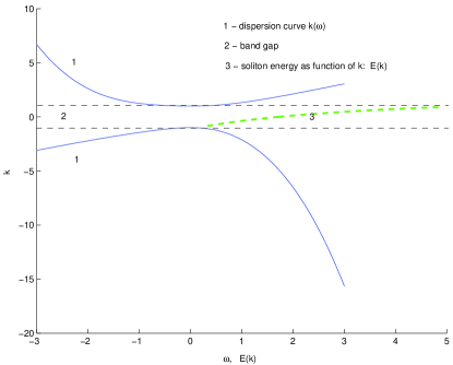
Figure 1: The solid curves are two branches of the dispersion relation (Gap solitons in a model of a hollow optical fiber), for $c=1$, $\gamma=0.3$. The bandgap is located between the branches. The bold dashed curve inside the bandgap shows the dependence $E(k)$ for the soliton family found in the gap. As is seen, the family fills the entire bandgap, and it always satisfies the VK stability condition, $dE/dk>0$.

In the gap, stationary soliton solution were sought for by the substitution of $\left\{u(z,\tau),v(z,\tau)\right\}=\left\{U(\tau;k),V(\tau;k)\right\}\exp\left(ikz\right)$ in Eqs. (1) and (2) and solving the resulting ODEs by means of the relaxation numerical method. Note that the functions $U$ and $V$ in this ansatz cannot be assumed real; however, they obey symmetry restrictions, so that $\mathrm{Re}\left(U(\tau)\right)$ and $\mathrm{Re}\left(V(\tau)\right)$ are even functions of $\tau$, while $\mathrm{Im}\left(U(\tau)\right)$ and $\mathrm{Im}\left(V(\tau)\right)$ are odd. Stability of the GS solutions was then tested in direct simulations. Additionally, it was tested by means of the Vakhitov-Kolokolov (VK) criterion VK : for the soliton family, the condition for the stability against perturbations with real eigenvalues is $dE/dk>0$, where the energy is

$$E(k)=\int_{-\infty}^{+\infty}\left[\left|U(\tau;k)\right|^{2}+\left|V(\tau;k)\right|^{2}\right]d\tau.$$ (4)

As a result, it has been concluded that the entire bandgap is filled by the solitons, and they all are stable in direct simulations (extensive scanning of the parameter space has not turned up any example of an unstable soliton). Besides that, all the GSs satisfy the VK criterion, see Fig. 1. A typical shape of the stationary GS is displayed in Fig. 2, and its stability against finite perturbations is illustrated by Fig. 3.

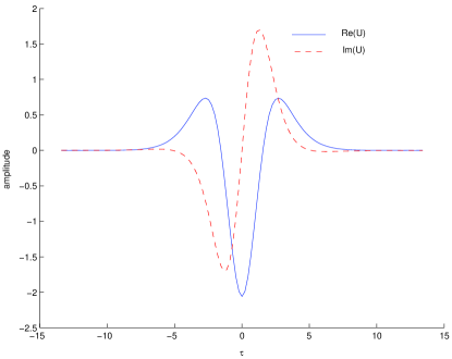
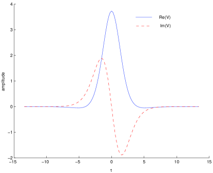
Figure 2: A generic example of the gap soliton (with $k=0$   and $\delta=0$) found inside the bandgap shown in Fig. 1. Note that the absolute values of the fields, $\left|U(\tau)\right|$ and $\left|V(\tau)\right|$, always have an ordinary single-humped shape.

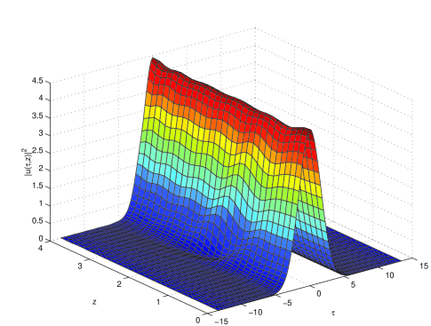
Figure 3: Stable evolution of the soliton from Fig. 2, to which an arbitrary initial perturbation was added, whose amplitude is $2\%$ of the soliton’s amplitude. The evolution is of the field $\left|v(z,\tau)\right|$ is similar to that displayed here for $\left|u(z,\tau)\right|$.

A natural extension of the GS family is generated by lending the soliton a finite velocity, in the reference frame of Eqs. (1) and (2). Note that, as well as the ordinary GS model, the present one features no Galilean (or other) invariance that would generate moving solitons automatically. To develop this extension, we rewrite Eqs. (1) and (2) in the boosted reference frame, replacing the independent variables $\left(z,\tau\right)$ by $\left(z,\tau^{\prime}\equiv\tau-\delta~{}z\right)$, where $\delta$ is the velocity shift. The transformation replaces the terms $i\left(u_{z},v_{z}\right)$ by $i\left(u_{z}-\delta~{}u_{\tau},v_{z}-\delta~{}v_{\tau}\right)$ and, accordingly, in the dispersion relation (Gap solitons in a model of a hollow optical fiber) $k$ is replaced by $k+\delta~{}\omega$. As a result, the bandgap changes its shape with the increase of $\delta$.

Naturally, the gap closes when $|\delta|$ is too large, and it is necessary to find the corresponding maximum and minimum values of the velocity shift, $\delta_{\max}$ and $\delta_{\min}$, up to which the bandgap exists. Straightforward analysis of the dispersion relation demonstrates that $\delta_{\max}=c$, which has a simple explanation: the above transformation replaces the coefficient $c$ in Eq. (2) by $c-\delta$, and the gap closes down when this combination vanishes. The other limit value can be found numerically from the corresponding algebra. The final result is presented in Fig. 4, that shows $\delta_{\max}$ and $\delta_{\min}$ as functions of $c$ for given $\gamma$. A noteworthy feature of this diagram is that the gap-supporting region continues, for $\delta\neq 0$, to negative $c$.

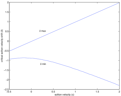
Figure 4: In the reference frame boosted by the velocity shift $\delta$, the bandgap exists in the interval $\delta_{\min}<\delta<\delta_{\max}\equiv c$. The two lines show $\delta_{\min}$ and $\delta_{\max}$ vs. $c$.

Solving the stationary equations in the boosted reference frame numerically, we have concluded that the entire gap is again completely filled with solitons. The boosted solitons obey the same symmetry constraints as in the case of $\delta=0$, so that the real and imaginary parts of the stationary fields are, respectively, even and odd functions of $\tau^{\prime}$. The fields $\left|u(z,\tau^{\prime})\right|$ and $\left|v(z,\tau^{\prime})\right|$ are always single-humped. A characteristic example of the boosted soliton in shown in Fig. 5. Finally, adding arbitrary initial perturbations shows that all the moving solitons are stable, in direct simulations, everywhere in the bandgap.

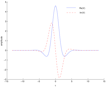
Figure 5: A generic example of the boosted gap soliton with $\delta=-0.5$, found at $c=0$ and $\gamma=0.3$. Note that, for $c=0$, the solitons with $\delta=0$ do not exist, see Fig. 4. In terms of $\left|u\right|$ and $\left|v\right|$, the boosted solitons always have a single-humped shape.

In conclusion, we have proposed the simplest model for two co-propagating waves in the hollow-core fiber, one a linear dispersionless core mode, and the other a dispersive nonlinear quasi-surface mode. The linear coupling between them may open a bandgap, through the mechanism of the crossing avoidance. The third-order dispersion of the latter mode is a necessary condition for the existence of the gap. The numerical results demonstrate that the entire bandgap is filled with solitons, and they all are stable in direct simulations. The gap-soliton (GS) family has been extended to include the boosted solutions, up to the limit values of the boost $\delta$ (these values are different for positive and negative $\delta$).

Solitons which were recently observed in hollow-core photonic-crystal fibers may belong to this GS family. The theoretical results suggest to extend the experimental study of these solitons, and of the “cutoff” solitons in hollow-core multilayer fibers, in order to identify their plausibly GS nature. On the other hand, the theoretical model needs to be extended by inclusion of the self-frequency shift and some other features. Results of the extension will be reported elsewhere.

After the submission of this paper for publication, a work by D.V. Skryabin, Opt. Exp. 12, 4841 (2004) has appeared, which considers a very similar model and also reports finding stable solitons in it.

References

- (1) W. Chen and D. L. Mills,Phys. Rev. Lett. 58,160(1987); D. L. Mills and S. E. Trullinger, Phys. Rev. B 36, 947 (1987).
- (2) A. B. Aceves and S. Wabnitz, Phys. Lett. A 141, 37 (1989); D. N. Christodoulides and R. I. Joseph, Phys. Rev. Lett. 62, 1746 (1989).
- (3) B. J. Eggleton et al., Phys. Rev. Lett. 76, 1627 (1996); C. M. de Sterke, B. J. Eggleton, and P. A. Krug, J. Lightwave Technol. 15, 1494 (1997).
- (4) C. M. de Sterke and J. E. Sipe, Progr. Opt. 33, 203 (1994); C. Conti, G. Assanto, and S. Trillo, J. Nonlin. Opt. Phys. Mat. 11, 239 (2002).
- (5) J. Feng, Opt. Lett. 18, 1302 (1993); R. F. Nabiev, P. Yeh, and D. Botez, Opt. Lett. 18, 1612 (1993); Yu. S. Kivshar, Phys. Rev. E 51, 1613 (1995);W. C. K. Mak, B.A. Malomed, and P. L. Chu, Phys. Rev. E 58, 6708 (1998); A. A. Sukhorukov and Yu. S. Kivshar, Opt. Lett. 27, 2112 (2002); I. M. Merhasin and B. A. Malomed, Phys. Lett. A 327, 296 (2004).
- (6) D. Mandelik et al., Phys. Rev. Lett. 90, 053902 (2003).
- (7) R. G. Scott et al., Phys. Rev. Lett. 90, 110404 (2003); B. Eiermann et al., Phys. Rev. Lett. 92, 230401 (2004).
- (8) R. F. Gregan et al., Science 285, 1537 (1999).
- (9) D. G. Ouzounov et al., Science 301 1702(2003).
- (10) F. Luan et al., Opt. Express 12, 835(2004).
- (11) W. Gobel, A. Nimmerjahn, and F. Helmchen, Opt. Lett. 29, 1285(2004).
- (12) H. Lim and F. W. Wise, Opt. Express 12, 2231(2004).
- (13) V. G. Bespalov, S. A. Kozlov, Y. A. Shpolyanskiy, and I. A. Walmsley, Phys. Rev. A 66, 013811 (2002).
- (14) C. M. Smith al., Nature 424, 657(2003).
- (15) K. Saitoh, N. A. Mortensen, and M. Koshiba, Opt. Express 12 394(2004).
- (16) E. Lidorikis, M. Soljăcić, Mi. Ibanescu, Y. Fink, and J. D. Joannopoulos, Opt. Lett. 29 851(2004).
- (17) Yu. S. Kivshar and G. P. Agrawal, Optical Solitons: From Fibers to Photonic Crystals (Academic Press: San Diego, 2003).
- (18) M. G. Vakhitov and A. A. Kolokolov, Radiophys. Quantum Electron. 16, 783 (1973).