Line Structures in Recurrence Plots

Abstract

Recurrence plots exhibit line structures which represent typical behaviour of the investigated system. The local slope of these line structures is connected with a specific transformation of the time scales of different segments of the phase-space trajectory. This provides us a better understanding of the structures occuring in recurrence plots. The relationship between the time-scales and line structures are of practical importance in cross recurrence plots. Using this relationship within cross recurrence plots, the time-scales of differently sampled or time-transformed measurements can be adjusted. An application to geophysical measurements illustrates the capability of this method for the adjustment of time-scales in different measurements.

,

1 Introduction

In the last decade of data analysis an impressive increase of the application of methods based on recurrence plots (RP) could be observed. Introduced by Eckmann et al. [1], RPs were firstly only a tool for the visualization of the behaviour of phase-space trajectories. The following development of a quantification of RPs by Zbilut and Webber [2, 3] and later by Marwan et al. [4], has consolidated the method as a tool in nonlinear data analysis. With this quantification the RPs have become more and more popular within a growing group of scientists who use RPs and their quantification techniques for data analysis. Last developments have extended the RP to a bivariate and multivariate tool, as the cross recurrence plot (CRP) or the multivariate recurrence plot (MRP) [5, 6, 7]. The main advantage of methods based on RPs is that they can also be applied to rather short and even nonstationary data.

The initial purpose of RPs was the visual inspection of higher dimensional phase space trajectories. The view on RPs gives hints about the time evolution of these trajectories. The RPs exhibit characteristic large scale and small scale patterns. Large scale patterns can be characterized as homogeneous, periodic, drift and disrupted. They obtain the global behaviour of the system (noisy, periodic, auto-correlated etc.). The quantification of RPs and CRPs uses the small-scale structures which are contained in these plots. The most important ones are the diagonal and vertical/horizontal straight lines because they reveal typical dynamical features of the investigated system, such as range of predictability or properties of laminarity. However, under a closer view a large amount of bowed, continuous lines can also be found. The progression of such a line represents a specific relationship within the data. In this paper we present a theoretical background of this relationship and discuss a technique to infer the adjustment of time-scales of two different data series. Finally, an example from earth siences is given.

2 Recurrence Plots

A recurrence plot (RP) is a two-dimensional squared matrix with black and white dots and two time-axes, where each black dot at the coordinates $(t_{1},t_{2})$ represents a recurrence of the system’s state $\vec{x}(t_{1})$ at time $t_{2}$:

$$\mathbf{R}(t_{1},t_{2})=\Theta\left(\varepsilon-\left\|\vec{x}(t_{1})-\vec{x}(t_{2})\right\|\right),\quad\vec{x}(t)\in\mathds{R}^{m},$$ (1)

where $m$ is the dimension of the system (degrees of freedom), $\varepsilon$ is a small threshold distance, $\|\cdot\|$ a norm and $\Theta(\cdot)$ the Heaviside function. This definition of an RP is only one of several possibilities (an overview of recent variations of RPs can be found in [8]).

Since $\mathbf{R}(t_{1},t_{1})=1$ by definition, the RP has a black main diagonal line, the line of identity (LOI), with an angle of $\pi/4$. It has to be noted that a single recurrence point at $(t_{1},t_{2})$ in an RP does not contain any information about the actual states at the times $t_{1}$ and $t_{2}$ in phase space. However, it is possible to reconstruct dynamical properties of the data from the totality of all recurrence points [9].

3 Line Structures in Recurrence Plots

The visual inspection of RPs reveals (among other things) the following typical small scale structures: single dots, diagonal lines as well as vertical and horizontal lines (the combination of vertical and horizontal lines plainly forms rectangular clusters of recurrence points).

Single, isolated recurrence points can occur if states are rare, if they do not persist for any time, or if they fluctuate heavily. However, they are not a clear-cut indication of chance or noise (for example in maps).

A diagonal line $\mathbf{R}(t_{1}+\tau,t_{2}+\tau)=1$ (for $\tau=1\dots l$, where $l$ is the length of the diagonal line in time units) occurs when a segment of the trajectory runs parallel to another segment, i. e. the trajectory visits the same region of the phase space at different times. The length of this diagonal line is determined by the duration of such a similar local evolution of the trajectory segments. The direction of these diagonal structures can differ. Diagonal lines parallel to the LOI (angle $\pi/4$) represent the parallel running of trajectories for the same time evolution. The diagonal structures perpendicular to the LOI represent the parallel running with contrary times (mirrored segments; this is often a hint of an inappropriate embedding if an embedding algorithm is used for the reconstruction of the phase-space). Since the definition of the Lyapunov exponent uses the time of the parallel running of trajectories, the relationship between the diagonal lines and the Lyapunov exponent is obvious (but this relationship is more complex than usually mentioned in literature, cf. [10]).

A vertical (horizontal) line $\mathbf{R}(t_{1},t_{2}+\tau)=1$ (for $\tau=1\dots v$, with $v$ the length of the vertical line in time units) marks a time length in which a state does not change or changes very slowly. It seems, that the state is trapped for some time. This is a typical behaviour of laminar states [4].

4 Slope of the Line Structures

In a more general sense the line structures in an RP exhibit locally the time relationship between the current trajectory segments. A line structure in an RP of length $l$ corresponds to the closeness of the segment $\vec{x}(T_{1}(t))$ to another segment $\vec{x}(T_{2}(t))$, where $T_{1}(t)$ and $T_{2}(t)$ are two local time-scales (or transformations of an imaginary absolute time-scale $t$) which preserve that $\vec{x}(T_{1}(t))\approx\vec{x}(T_{2}(t))$ for some time $t=1\dots l$. Under some assumptions (e. g. piecewise existence of an inverse of the transformation $T(t)$, the two segments visit the same area in the phase space), a line in the RP can be simply expressed by the time-transfer function

$$\vartheta(t)=T_{2}^{-1}\left(T_{1}(t)\right).$$ (2)

Especially, we find that the local slope $b(t)$ of a line in an RP represents the local time derivative $\partial_{t}$ of the inverse second time-scale $T_{2}^{-1}(t)$ applied to the first time-scale $T_{1}(t)$

$$b(t)=\partial_{t}T_{2}^{-1}\left(T_{1}(t)\right)=\partial_{t}\vartheta(t).$$ (3)

This is the fundamental relation between the local slope $b(t)$ of line structures in an RP and the time scaling of the corresponding trajectory segments. From the slope $b(t)$ of a line in an RP we can infere the relation $\vartheta(t)$ between two segments of $\vec{x}(t)$ ($\vartheta(t)=\int b(t)dt$). Note that the slope $b(t)$ depends only on the transformation of the time-scale and is independent from the considered trajectory $\vec{x}(t)$.

This feature is, e. g., used in the application of CRPs as a tool for the adjustment of time-scales of two data series [6, 11] and will be discussed later. Next, we present the deforming of line structures in RPs due to different transformations of the time-scale.

5 Illustration Line Structures

For illustration we consider some examples of time transformations for different one-dimensional trajectories $f(t)$ (i. e. functions; no embedding). We study the recurrence behaviour between two segments $f_{1}$ and $f_{2}$ of these trajectories, where we apply different time transformations to these segments (Tab. 1). In order to illustrate that the found relation (3) is independent from the underlying trajectory, we will use at first the function $f(t)=t^{2}$ (Figs. 1A1, B1, C1 etc.) and then $f(t)=\sin(\pi\,t)$ (Figs. 1A2, B2, C2 etc.) as a trajectory. The local representation of RPs between these segments corresponds finally to cross recurrence plots (CRP) between two different trajectories/functions as will be mentioned later.

Table 1: Examplary time transformation functions $T_{1}(t)$ and $T_{2}(t)$, the inverse $T_{2}^{-1}(t^{\prime})$, their corresponding slopes $b(t)$ and time-transfer functions $\vartheta(t)$ for lines in RPs shown in Fig. 1.

Fig.	$T_{1}(t)$	$T_{2}(t)$	$T_{2}^{-1}(t^{\prime})$	$b(t)$	$\vartheta(t)$
A	$t$	$2t$	$0.5\,t^{\prime}$	$0.5$	$0.5\,t$
B	$t$	$5t^{2}$	$\sqrt{0.2\,t^{\prime}}$	$\sqrt{\frac{0.2}{t}}$	$\sqrt{0.2\,t}$
C	$t$	$\sqrt{1-t^{2}}$	$\sqrt{1-t^{\prime 2}}$	$\frac{t}{\sqrt{1-t^{2}}}$	$\sqrt{1-t^{2}}$
D	$t^{2}$	$t^{3}$	$\sqrt[3]{t^{\prime}}$	$\frac{1}{3\sqrt[3]{t^{2}}}$	$\sqrt[3]{t^{2}}$
E	$\sin(\pi\,t)$	$t^{3}$	$\sqrt[3]{t^{\prime}}$	$\frac{\pi\,\cos(\pi\,t)}{3\sqrt[3]{\sin^{2}(\pi\,t)}}$	$\sqrt[3]{sin(\pi\,t)}$

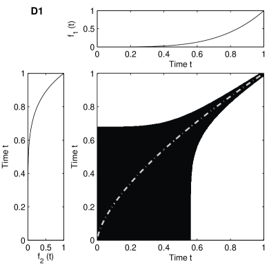
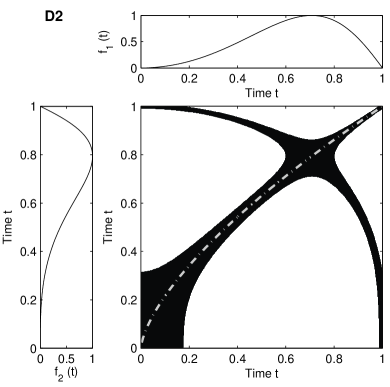
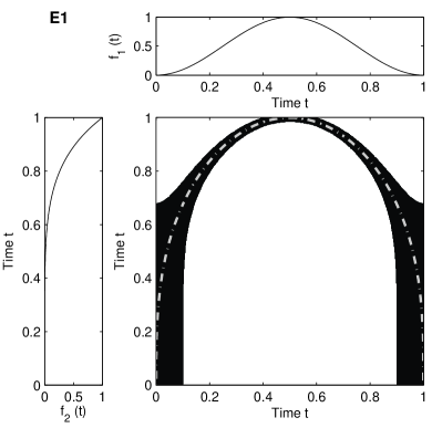
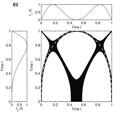
Figure 1: Details of recurrence plots for trajectories $f(t)$ whose sub-sections $f_{1}(t)$ and $f_{2}(t)$ undergo different transformations in time-scale (Tab. 1). Black areas correspond to times where $f_{1}(t)\approx f_{2}(t)$. The dash-dotted lines represent the time-transfer functions $\vartheta(t)$. Note that these are not the entire RPs, only a small detail of them (an entire RP cannot contain only these structures – there are more features, like the line of identity (diagonal line from lower left to upper right) and a more or less symmetric plot around this line).

Assuming that the second segment of a trajectory $f_{2}$ is twice as fast as the first segment $f_{1}$ (Figs. 1A), i. e., the time transformations are $T_{1}(t)=t$ and $T_{2}(t)=2t$, we get a constant slope $b=0.5$ by using Eq. (3). A line in an RP which corresponds to these both segements follows $\vartheta(t)=0.5\,t$ (Figs. 1A1, A2). This result corresponds with the solution we had already discussed in [11] using another approach. In [11] we considered a simple case of two harmonic functions $f_{1}(t)=\sin(T_{1}(t))$ and $f_{2}(t)=\sin(T_{2}(t))$ with different time transformation functions $T_{1}=\varphi\cdot t+\alpha$ and $T_{2}=\psi\cdot t+\beta$. Using the inverse $T_{2}^{-1}=\frac{t-\beta}{\psi}$ and Eq. (3), we get the local slope of lines in the RP (or CRP) $b=\partial_{t}T_{2}^{-1}\left(T_{2}(t)\right)=\varphi/\psi,$ which equals the ratio between the frequencies of the considered harmonic functions.

In the second example we will transform the time-scale of the second segment with the square function $T_{2}(t)=5t^{2}$. Using Eq. (3) we get $b(t)=\sqrt{0.2/t}$ and $\vartheta(t)=\sqrt{0.2\,t}$, which corresponds with a bowed line in the RP (Figs. 1B1, B2). Since $\sin(\pi\,x)$ has some periods in the considered intervall, we get some more lines in the RP (Figs. 1B2). These lines underly the same relationship, but we have to take higher periodicities into account: $\vartheta(t)=\sqrt{0.2\,k\,\pi\,t}$ ($k\in\mathds{Z}$).

The third example refers to a hyperbolic time transformation $T_{2}(t)=\sqrt{1-t^{2}}$. The resulting line in the RP has the slope $b(t)=t/\sqrt{1-t^{2}}$ and follows $\vartheta(t)=\sqrt{1-t^{2}}$, which corresponds with a segment of a circle (Figs. 1C1, C2). We can use this information in order to create a full circle in an RP. Let us consider a one-dimensional system, where the trajectory is simply the function $f(T)=T(t)$, and with a section of a monotonical, linear increase $T_{lin}=t$ and another (hyperbolic) section which follows $T_{hyp}=-\sqrt{r^{2}-t^{2}}$. After these both sections we append the same but mirrored sections (Fig. 2A). Since the inverse of the hyperbolic section is $T_{hyp}^{-1}=\pm\sqrt{r^{2}-t^{2}}$, the line in the corresponding RP follows $\vartheta(t)=T_{hyp}^{-1}(T_{lin}(t))=\pm\sqrt{r^{2}-t^{2}}$, which corresponds with a circle of radius $r$ (Fig. 2B).

An examplary data series from earth science reveals that such structures are not only restricted to artificial models. Let us consider the January solar insolation for the last 100 kyr on the latitude 44^∘N (Fig. 3A). The corresponding RP shows a circle (Fig. 3B), similar as in Fig. 2B. From this geometric structure we can infer that the insolation data contains a more-or-less symmetric sequence and that subsequent sequences are equal after a suitable time transformation which follows the relation $T_{2}^{-1}(T_{1})=\sqrt{r^{2}-t^{2}}$. For instance, the subsequent sequences could be a linear increasing and a hyperbolic decreasing followed by a reverse of this sequence, a hyperbolic increasing and a linear decreasing part. Such bowed line structures can also be found in RPs applied to data from biology, ecology, economy. These deformations can obtain hints about the change of frequencies during the evolution of a process and may be of major interest especially in the analysis of sound data (an example of an RP of speech data containing pronounced bowed lines can be found in [12]).

Whereas in the examples above only the second section of the trajectory undergoes a time transformation, in the last two examples (Figs. 1D and E) the time-scale of the first section is also transformed. Nevertheless, the time-transfer function can be again determined with Eq. (2) too.

From these examples we can conclude that the line in a recurrence plot follows Eq. (2) and depends only on the transformations of the time-scale.

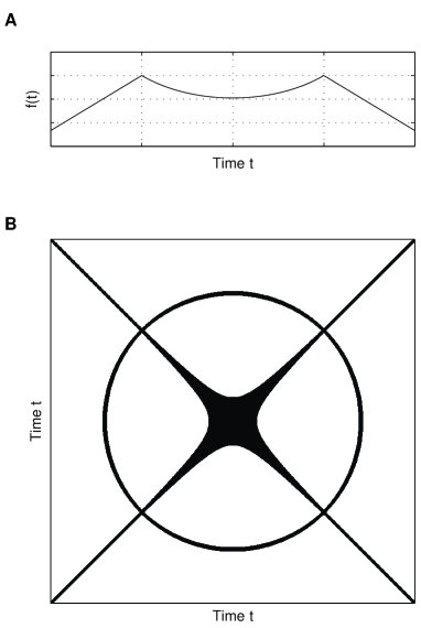
Figure 2: Illustrative example of the relationship between the slope of lines in an RP and the local derivatives of the involved trajectory segments. Since the local derivative of the transformation of the time-scales of the linear and the hyperbolic sections (A) corresponds to the derivative of a circle line, a circle occurs in the RP (B). Recurrence plot is derived from the one-dimensional phase-space (no embedding used).

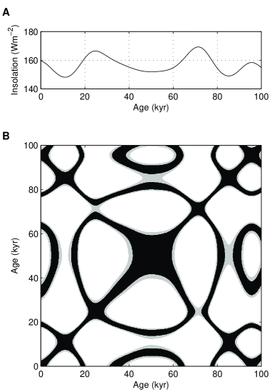
Figure 3: A corresponding structure found in experimental data: (A) the solar insolation on the latitude 44^∘N for the last 100 kyr (data from [13]) and its corresponding recurrence plot (B). The recurrence plot parameters were $m=1$ and $\varepsilon=2$ (black) and $\varepsilon=3.5$ (gray).

6 Cross Recurrence Plots

The relationship between the local slope of line structures in RPs and the corresponding different segments of the same phase-space trajectory holds also for the structures in CRPs,

$$\mathbf{CR}(t_{1},t_{2})=\Theta\bigl{(}\varepsilon-\left\|\vec{x}(t_{1})-\vec{y}(t_{2})\right\|\big{)}.$$ (4)

which are based on two different phase-space trajectories $\vec{x}(t_{1})$ and $\vec{y}(t_{2})$. This relationship is more important for the line of identity (LOI) which then becomes a line of synchronization (LOS) in a CRP [6, 11].

We start with two identical trajectories, i. e. the CRP is the same as the RP of one trajectory and contains an LOI. If we now slightly modify the amplitudes of the second trajectory, the LOI will become somewhat disrupted. This offers a new approach to use CRPs as a tool to assess the similarity of two systems [5]. However, if we do not modify the amplitudes but stretch or compress the second trajectory slightly, the LOI will remain continuous but not as a straight line with an angle of $\pi/4$. The line of identity (LOI) now becomes the line of synchronization (LOS) and may eventually not have the angle $\pi/4$. This line can be rather bowed. Finally, a time shift between the trajectories causes a dislocation of the LOS, hence, the LOS may lie rather far from the main diagonal of the CRP.

Now we deal with a situation which is typical in earth sciences and assume that two trajectories represents the same process but contain some transformations in their time-scales. The LOS in the CRP between the two trajectories can be described with the found relation (2). The function $\vartheta(t)$ is the transfer or rescaling function which allows to readjust the time-scale of the second trajectory to that of the first one in a non-parametrical way. This method is useful for all tasks where two time-series have to be adjusted to the same scale, as in dendrochronology or sedimentology [6].

Next, we apply this technique in order to re-adjust two geological profiles (sediment cores) from the Italian lake Lago di Mezzano [14]. The profiles cover approximately the same geological processes but have different time-scales due to variations in the sedimentation rates. The first profile (LMZC) has a length of about 5 m and the second one (LMZG) of about 3.5 m (Fig. 4). From both profiles a huge number of geophysical and chemical parameters were measured. Here we focus on the rock-magnetic measurements of the normalized remanent magnetization intensity (NRM) and the susceptibility $\kappa$.

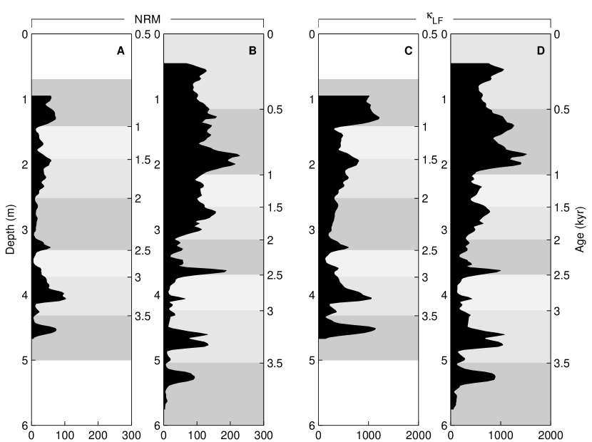
Figure 4: Rock-magnetic measurements of lake sediments with different time-scales. Corresponding sections are marked with different gray values.

We use the time-series NRM and $\kappa$ as components for the phase-space vector, resulting in a two-dimensional system. However, we apply an additional embedding using the time-delay method [15] (we do not ask about the physical meaning here). A rather small embedding decreases the amount of line structures representing the progress with negative time [8]. Using embedding parameters dimension $m=3$ and delay $\tau=5$ (empirically found for these time-series), the final dimension of the reconstructed system is six. The corresponding CRP reveals a partly disrupted, swollen and bowed LOS (Fig. 5). This LOS can be automatically resolved, e. g. by using the LOS-tracking algorithm as described in [11]. The application of this LOS as the time-transfer function to the profile LMZG re-adjusts its time-series to the same time-scale as LMZC (Fig. 6). This method offers a helpful tool for an automatic adjustment of different geological profiles, which offers advantages compared to the rather subjective method of ”wiggle matching” (adjustment by harmonizing maxima and minima by eye) used so far.

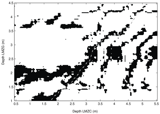
Figure 5: Cross recurrence plot between rock-magnetic data shown in Fig. 4. The dash-dotted line is the resolved LOS which can be used for re-adjustment the time-scales of both data sets.

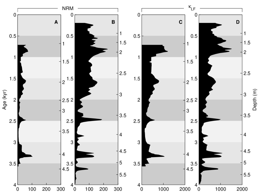
Figure 6: Geological profiles after re-adjustment using the LOS which was found with the CRP shown in Fig. 5. Corresponding sections are marked with different gray values.

7 Conclusion

Line structures in recurrence plots (RPs) and cross recurrence plots (CRPs) contain information about epochs of a similar evolution of segments of phase-space trajectories. Moreover the local slope of such line structures is directly related with the difference in the velocity the system changes at different times. We have demonstrated that the knowlege about this relationship allows a better understandig of even bowed structures occuring in RPs. This relationship can be used to analyse changes in the time domain of data series (e. g. frequencies), as it is of major interest, e. g., in the analysing of speech data. We have used this feature in a CRP based method for the adjustment of time-scales between different time-series. The potential of this technique is finally shown for experimental data from geology.

8 Acknowledgements

This work was partly funded or supported by the Special Research Programmes SPP1097 and SPP1114 of the German Science Foundation (DFG) as well as by the project AO-99-030 of European Space Agency. We gratefully acknowledge N. Nowaczyk and U. Frank (GeoForschungsZentrum Potsdam) for the helpful discussions and for providing the geophysical data. The recurrence plots and cross recurrence plots were created by using the CRP toolbox for Matlab (http://tocsy.agnld.uni-potsdam.de).

References

- [1] J.-P. Eckmann, S. O. Kamphorst, D. Ruelle, Recurrence Plots of Dynamical Systems, Europhysics Letters 5 (1987) 973–977.
- [2] J. P. Zbilut, C. L. Webber Jr., Embeddings and delays as derived from quantification of recurrence plots, Physics Letters A 171 (3–4) (1992) 199–203. doi:10.1016/0375-9601(92)90426-M
- [3] C. L. Webber Jr., J. P. Zbilut, Dynamical assessment of physiological systems and states using recurrence plot strategies, Journal of Applied Physiology 76 (2) (1994) 965–973.
- [4] N. Marwan, N. Wessel, U. Meyerfeldt, A. Schirdewan, J. Kurths, Recurrence Plot Based Measures of Complexity and its Application to Heart Rate Variability Data, Physical Review E 66 (2) (2002) 026702. doi:10.1103/PhysRevE.66.026702
- [5] N. Marwan, J. Kurths, Nonlinear analysis of bivariate data with cross recurrence plots, Physics Letters A 302 (5–6) (2002) 299–307. doi:10.1016/S0375-9601(02)01170-2
- [6] N. Marwan, J. Kurths, Cross recurrence plots and their applications, in: C. V. Benton (Ed.), Mathematical Physics Research at the Cutting Edge, Nova Science Publishers, Hauppauge, 2004, pp. 101–139.
- [7] M. Romano, M. Thiel, J. Kurths, W. von Bloh, Multivariate Recurrence Plots, Physics Letters A 330 (3–4) (2004) 214–223. doi:10.1016/j.physleta.2004.07.066
- [8] N. Marwan, Encounters With Neighbours – Current Developments Of Concepts Based On Recurrence Plots And Their Applications, Ph.D. thesis, University of Potsdam (2003).
- [9] M. Thiel, M. C. Romano, J. Kurths, How much information is contained in a recurrence plot?, Physics Letters A 330 (5) (2004) 343–349. doi:10.1016/j.physleta.2004.07.050
- [10] M. Thiel, M. C. Romano, P. L. Read, J. Kurths, Estimation of dynamical invariants without embedding by recurrence plots, Chaos 14 (2) (2004) 234–243. doi:10.1063/1.1667633
- [11] N. Marwan, M. Thiel, N. R. Nowaczyk, Cross Recurrence Plot Based Synchronization of Time Series, Nonlinear Processes in Geophysics 9 (3/4) (2002) 325–331.
- [12] R. Hegger, H. Kantz, L. Matassini, Denoising Human Speech Signals Using Chaoslike Features, Physical Review Letters 84 (14) (2000) 3197–3200. doi:10.1103/PhysRevLett.84.3197
- [13] A. Berger, M. Loutre, Insolation values for the climate of the last 10 million years, Quaternary Science Reviews 10 (4) (1991) 297–317. doi:10.1016/0277-3791(91)90033-Q
- [14] U. Brandt, N. R. Nowaczyk, A. Ramrath, A. Brauer, J. Mingram, S. Wulf, J. F. W. Negendank, Palaeomagnetism of holocene and late pleistocene sediments from lago di mezzano and lago grande di monticchio (italy): Initial results, Quaternary Science Reviews 18 (7) (1999) 961–976. doi:10.1016/S0277-3791(99)00008-6
- [15] J. Theiler, S. Eubank, A. Longtin, B. Galdrikian, B. Farmer, Testing for nonlinearity in time series: the method of surrogate data, Physica D 58 (1992) 77–94. doi:10.1016/0167-2789(92)90102-S