Standing Waves in a Non-linear 1D Lattice : Floquet Multipliers, Krein Signatures, and Stability

Abstract

We construct a class of exact commensurate and incommensurate standing wave (SW) solutions in a piecewise smooth analogue of the discrete non-linear Schrödinger (DNLS) model and present their linear stability analysis. In the case of the commensurate SW solutions the analysis reduces to the eigenvalue problem of a transfer matrix depending parametrically on the eigenfrequency. The spectrum of eigenfrequencies and the corresponding eigenmodes can thereby be determined exactly. The spatial periodicity of a commensurate SW implies that the eigenmodes are of the Bloch form, characterised by an even number of Floquet multipliers. The spectrum is made up of bands that, in general, include a number of transition points corresponding to changes in the disposition of the Floquet multipliers. The latter characterise the different band segments. An alternative characterisation of the segments is in terms of the Krein signatures associated with the eigenfrequencies. When one or more parameters characterising the SW solution is made to vary, one occasionally encounters collisions between the band-edges or the intra-band transition points and, depending on the the Krein signatures of the colliding bands or segments, the spectrum may stretch out in the complex plane, leading to the onset of instability. We elucidate the correlation between the disposition of Floquet multipliers and the Krein signatures, presenting two specific examples where the SW possesses a definite window of stability, as distinct from the SW’s obtained close to the anticontinuous and linear limits of the DNLS model.

,

1 Introduction

The question of enumerating and classifying the possible excitations in a discrete non-linear lattice (e.g., a Fermi-Pasta-Ulam(FPU) chain) is too complex to be even addressed in its entirety. However, important classes of excitations have already been identified and studied exhaustively, and their physical implications are in the process of being worked out. One such class consists of localised solutions, namely the discrete breathers with periodic or quasi-periodic time-variation, while a related class includes the travelling breather solutions. A third class of solutions can be described as non-linear spatially periodic travelling waves analogous to the phonon modes in linear lattices. The existence of such travelling waves has been established in non-linear discrete Klein-Gordon (NDKG) lattices as well as in FPU chains ref1 ; ref2 close to the linear limit (i.e., for small amplitudes) as also in the vicinity of the so called anti-continuous limit (small inter-site coupling). In the latter case, the travelling waves were constructed as an infinite array of breathers (multi-breathers) with an appropriate phase introduced at each breather site.

More recently, commensurate and incommensurate standing wave (SW) solutions have also been investigated in the literature, once again close to the two limits referred to above ref3 ; ref4 . Close to the linear limit, small amplitude SW solutions in the NDKG chain have been obtained from the DNLS approximation by referring to orbits in a small neighbourhood of a fixed point in a related area-preserving mapping. In the weak-coupling situation, on the other hand, one obtains the SW solutions by continuation from the anti-continuous limit of a solution with an appropriate coding sequence. In either of these approaches one can obtain SW solutions both commensurate and incommensurate with the underlying lattice. Even chaotic spatial structures are not ruled out.

The question of stability of these standing wave solutions is a more complex one. In the case of the travelling waves, it appears that they are afflicted with a type of modulational instability, as a result of which they break up into an array of localised pulses. The SW’s in general also happen to be linearly unstable close to the small amplitude limit. For the commensurate SW’s the eigenfrequencies form bands on the real axis, but these bands have a tendency to overlap and extend into the complex plane leading to oscillatory instabilities for arbitrarily small amplitudes. The spectra for incommensurate SW’s, on the other hand, are generaly cantor-like and require a more sophisticated analysis ref3 ; ref4 , but here again one finds that the SW’s with even arbitrarily small amplitudes are prone to oscillatory instability.

In the present paper we present an exact construction of commensurate and incommensurate SW’s in a piece-wise smooth (PWS) system resembling the DNLS model and perform an exact linear stability analysis for the commensurate SW’s. The linearised evolution equation for an SW in the model depends essentially on two parameters - the breather frequency $\omega$ and a nonlinearity parameter $\gamma$ and, in contrast to breathers obtained perturbatively from the linear limit, one can identify well-defined regions in the $\omega$-$\gamma$ parameter space where the SW’s are linearly stable. In other words, away from the linear and anti-continuous limits there do exist stable commensurate SW solutions - the main result of this paper. In addition, the bands of eigenfrequencies arising from the linearised evolution equation which we calculate in arriving at the stability result present interesting features. While in general there exist gaps between the edges of successive bands and the width of the band gaps varies with the parameters $\omega,~{}\gamma$, instability does not necessarily occur through a collision of the band-edges (i.e., shortening of a band-gap to zero width). As we shall see, there may exist, in addition to the band-edges, a number of transition points (see below) within the bands and collisions of these intra-band transition points may equally well account for the onset of instabilty. The model under consideration being explicitly solvable, the detailed structure of a band can be worked out, including the location of the band-edges and transition points as also the eigenmodes associated with the different band segments. Additionally, the different band segments can be characterised in terms of the Krein signatures ref5 ; ref6 ; ref7 associated with the eigenfrequencies, and the correlation between the various possible dispositions of Floquet multipliers (see below) and the Krein signatures can be looked at. This gives us insight into infinite dimensional linear Hamiltonian systems with Bloch type eigenfunctions in the context of the theory of Hamiltonian Hopf bifurcation ref8 ; ref9 ; ref10 in infinite dimensional systems (see also ref7 ).

In section 2 below, we present the piecewise smooth DNLS model and briefly recall results from a couple of earlier papers LPR1 ; LPR2 relating to the single-site and multi-site breather solutions. Section 3 presents the exact commensurate and incommensurate SW solutions, obtained by extension of the multi-site breathers where the breathers form an infinitely extended periodic or quasiperiodic array. Section 4 is devoted to the formulation of the stability problem with special reference to the commensurate SW solutions where the problem of calculating the spectrum of eigenfrequencies is reduced to the consideration of the eigenvalue problem of a $4\times 4$ complex transfer matrix depending parametrically on the eigenfrequency $p$ of the original problem as also on the breather parameters $\lambda$ (related to the breather frequency $\omega$), $\gamma$. We indicate how the bands, together with their edges and transition points, are determined by the parametric bifurcation of the transfer matrix. This section also elucidates the correlation between the Floquet multipliers and the Krein signatures associated with the different band segments in the context of the linearised variational equations which constitute an infinite dimensional linear Hamiltonian system, and their role in characterising the onset of instability. In section 5, we specialise to a couple of particular cases involving SW’s with specified spatial periodicity and phase characteristics. In both these cases the onset of instability is associated with a collision among intra-band transition points, and we obtain explicitly the window of stability in the $\lambda$-$\gamma$ plane. This section also contains concluding remarks.

2 Breather solutions in a DNLS-like model

In LPR1 ; LPR2 we considered a piecewise smooth DNLS-like model given by

$$i\frac{d\psi_{n}}{dt}+(\psi_{n+1}+\psi_{n-1})+f(|\psi_{n}|)\psi_{n}=0,$$ (1a)

with

$$f(x)=\gamma(1-\frac{1}{x})\ominus(x-1),$$ (1b)

where $\ominus$ stands for the Heavyside step function and $\gamma$ is a parameter characterising the strength of non-linearity. The non-linear term also involves a threshold parameter which we have scaled to unity. With reference to this threshold parameter we characterise lattice sites as being either high or low depending on whether $|\psi_{n}|>1$ or $|\psi_{n}|<1$ respectively. As indicated in LPR1 ; LPR2 the model is qualitatively similar to the cubic DNLS model (though the latter does not explicitly involve a threshold parameter) and possesses breather solutions of similar features. In particular, we presented explicit construction of single site and two-site breathers as also an explicit stability analysis of these breathers.

The single site breather solution is characterised by two parameters : a spatial decay rate $\lambda$ (related to the breather frequency as $\omega=-\lambda-\frac{1}{\lambda}$) and the nonlinearity parameter $\gamma$, and is given by

$$\psi_{n}={\bar{\phi}}_{n}e^{-i\omega t},$$ (2a)

$${\bar{\phi}}_{n}=\frac{\gamma}{\gamma+\lambda-\frac{1}{\lambda}}\lambda^{|n|}.$$ (2b)

The parameter $\gamma$ is to be larger than a certain threshold value (depending on $\lambda$) for this breather solution to exist. The linearisation of (1a), (1b) around (2a), (2b) in the rotating frame was then shown to possess a spectrum consisting of a single band with extended eigenmodes and an isolated point corresponding to a localised mode (in addition to a trivial phase mode with eigenfrequency zero). As the parameters $\lambda$ and $\gamma$ are made to vary, the isolated point in the spectrum gets shifted while the band remains fixed in the frequency scale and, as a certain stability border in the $\lambda$-$\gamma$ plane is crossed, the isolated point in the spectrum approaches zero (the ‘double-zero’ configuration) with a consequent onset of stationary instability. Interestingly, there exists a certain critical value of the spatial decay rate $(\lambda_{c})$ above which the breather becomes intrinsically unstable.

In LPR2 the model was also shown to possess $2$-site monochromatic breather solutions of the form (2a) with high sites located at, say, $n=0$ and $n=N$, the amplitude at the high sites being

$$b=\frac{\gamma(1-\lambda^{2N})}{\gamma(1-\lambda^{2N})-(\frac{1}{\lambda}-\lambda)(1-\lambda^{N}e^{i\delta})}.$$ (3)

Here $\delta$ is the phase difference between the two high sites, which can be either $0$ or $\pi$, and once again $\gamma$ is to be larger than a certain threshold value depending on $\lambda$ for the breather to exist. An exact linear stability analysis was performed for the two-site breathers. The in-phase breather $(\delta=0)$ was found to be intrinsically unstable while, for anti-phase breather ($\delta=\pi$), one obtains a band of extended modes together with a pair of localised symmetric modes and another pair of localised antisymmetric modes for parameters $(\lambda,\gamma)$ away from a stability border (for given $N$). As the parameters are made to vary, the isolated eigenfrequencies get shifted and, at the stability border the breather is destabilised through a Krein collision involving the symmetric eigenmodes.

The model (1a),(1b) admits of many other breather solutions including, possibly, spatially random ones. We present below a class of exact commensurate and incommensurate standing wave (SW) solutions in the model and then perform their linear stability analysis, with special reference to the commensurate SW’s.

3 Commensurate and Incommensurate SW solutions

We consider a class of breather solutions for which the high sites are located in a periodic array at $n=0,\pm N,\pm 2N,\pm 3N,\ldots$. However, successive high sites are allowed a phase difference $\delta$ that may or may not be a rational multiple of 2$\pi$ (cf. the $2$-site breather solution where $\delta$ is either 0 or $\pi$). In between the high sites there occurs a succession of low sites where one has

$$i\frac{d\psi_{n}}{dt}+(\psi_{n+1}+\psi_{n-1})=0.$$ (4)

Considering monochromatic breathers of the form (2a), (4) gives

$${\bar{\phi}}_{n}=\alpha\lambda^{n}+\beta\lambda^{-n},$$ (5)

where $\lambda$ satisfies

$$\lambda+\frac{1}{\lambda}=-\omega,$$ (6)

and where we choose without loss of generality $|\lambda|<1$. Note that $|\omega|>2$, i.e., the breather frequency lies outside the linear phonon band. In the following we restrict ourselves to $\lambda>0$ ($\omega<-2$) for the sake of concreteness (corresponding results are obtained for $\lambda<0$).

To be more specific, we look for monochromatic SW solutions of the form (2a) where high sites are located in a periodic array on the lattice at, say, $n=0,\pm N,\pm 2N,\ldots(N\geq 2)$. Each high site is flanked on either side by a low site and the magnitude $|\psi_{n}|$ at each high site is the same, say, $b$. However, we allow for a phase difference $\delta$ between successive high sites. We note from (1a), (1b) that for a low site (i.e., one with $|\psi_{n}|<1$),

$${\bar{\phi}}_{n}+{\bar{\phi}}_{n+1}+{\bar{\phi}}_{n-1}=0,$$ (7)

i.e., ${\bar{\phi}}_{n}$ is of the form (5), where $\lambda$ satisfies (6) and $\alpha$, $\beta$ are appropriate constants. For a high site with $|\psi_{n}|=b>1$, on the other hand,

$$\omega be^{i\theta_{n}}+{\bar{\phi}}_{n+1}+{\bar{\phi}}_{n-1}=-\gamma be^{i\theta_{n}}(1-\frac{1}{b}),$$ (8)

where $\theta_{n}$ denotes the phase at the site under consideration. Taking together all these requirements, one arrives at the following SW solution:

$${\bar{\phi}}_{kN+m}=be^{ik\delta}\left(\frac{1-e^{i\delta}\lambda^{N}}{1-\lambda^{2N}}\lambda^{m}+\frac{e^{i\delta}-\lambda^{N}}{1-\lambda^{2N}}\lambda^{N-m}\right),$$ (9)

where the index $n$ for a site has been expressed in the form

$$n=kN+m~{}~{}(0\leq m<N,~{}~{}k=0,\pm 1,\pm 2,\ldots),$$ (10)

with $k,m$ integers determined uniquely by $n$ (for given $N$). Note that, while the phase advance $(\delta)$ is uniform between successive high sites $(n=kN,n=(k+1)N)$, it is not necessarily so for arbitrarily chosen pairs of successive sites $n,n+1$.

It is also important to note that the standing wave solution (2a), (9) is valid only if $\gamma,~{}\omega$ satisfy appropriate constraints corresponding to the consistency conditions

$$|{\bar{\phi}}_{0}|>1,~{}~{}~{}~{}~{}|{\bar{\phi}}_{1}|<1,$$ (11)

which imply, in general, that $\gamma$ is to be larger than a certain threshold value $\gamma_{1}(\lambda)$ depending on $N$ and $\delta$ (as already mentioned, similar conditions also apply for single-site and two-site breathers obtained in LPR1 ; LPR2 ). Expressions of $\gamma_{1}(\lambda)$ for the particular cases $N=2,~{}\delta=\pi$, and also for $N=3,~{}\delta=\pi$, will be found below.

Evidently, (9) represents a spatially periodic, or commensurate standing wave solution if $\delta$ is a rational multiple of $2\pi$, say, $\delta=(\frac{r}{q})2\pi$ ($r,~{}q$, co-prime integers, $q>0$), in which case both the amplitude and phase are repeated at intervals of $\tilde{N}=qN$ lattice sites. On the other hand, if $\frac{\delta}{2\pi}$ is irrational, (9) represents an incommensurate standing wave since the phase of $\psi_{n}$ never repeats itself, but comes arbitrarily close to any preassigned value $\bar{\delta}$ for some $n$ or other.

In section (5), we consider for the sake of concreteness two particular commensurate solutions with $\delta=\pi$ and with $N=2,~{}3$ respectively. The solution for $N=2,~{}\delta=\pi~{}(\tilde{N}=4)$ reads (up to translation by a lattice site)

$${\bar{\phi}}_{0}=-{\bar{\phi}}_{2}=b,$$ (12a)

$${\bar{\phi}}_{1}={\bar{\phi}}_{3}=0,$$ (12b)

$${\bar{\phi}}_{n+\tilde{N}}={\bar{\phi}}_{n},$$ (12c)

where

$$b=\frac{\gamma}{\gamma+\omega},$$ (12d)

and where $$\gamma$$ is to satisfy the consistency condition

$$\gamma>\gamma_{1}(\lambda)|_{N=2,~{}\delta=\pi}=-\omega.$$ (12e)

Recall that in this paper we restrict to $\omega<-2$, while similar results are obtained for $\omega>2$. In a similar manner, one has, for $N=3$, $\delta=\pi$ (periodicity $\tilde{N}=6$)

$${\bar{\phi}}_{0}=-{\bar{\phi}}_{3}=b,$$ (13a)

$${\bar{\phi}}_{1}=-{\bar{\phi}}_{2}=-{\bar{\phi}}_{4}={\bar{\phi}}_{5}=\frac{b}{1-\omega},$$ (13b)

$${\bar{\phi}}_{n+\tilde{N}}={\bar{\phi}}_{n},$$ (13c)

where

$$b=\frac{\gamma~{}(1-\lambda^{3})}{\gamma~{}(1-\lambda^{3})-\frac{1-\lambda^{2}}{\lambda}(1+\lambda^{3})},$$ (13d)

and where

$$\gamma>~{}\gamma_{1}(\lambda)|_{N=3,\delta=\pi}~{}=\frac{1+\lambda+\lambda^{3}+\lambda^{4}}{\lambda+\lambda^{3}}.$$ (13e)

Having obtained the commensurate and incommensurate standing waves in our piecewise smooth DNLS-like model, we now turn to their linear stability analysis.

4 Linear Stability Analysis

4.1 The transfer matrix

We consider a perturbation $u_{n}$ over the breather profile ${\bar{\phi}}_{n}$ of (2a), (9), (10) in the rotating frame and write (we drop the bar over $\phi_{n}$)

$$\psi_{n}=(\phi_{n}+u_{n}(t))e^{-i\omega t}.$$ (14)

Using this in (1a), (1b) and linearising, one obtains

$$i\dot{u}_{n}+\omega u_{n}+u_{n+1}+u_{n-1}=-\gamma\{u_{n}-\frac{\phi_{n}}{2|\phi_{n}|}(\frac{u_{n}}{\phi_{n}}-\frac{u_{n}^{*}}{\phi_{n}^{*}})\}\ominus(|\phi_{n}|-1).$$ (15)

This actually represents a linear Hamiltonian system, and we seek a harmonic solution of the form

$$u_{n}(t)=a_{n}e^{ipt}+b_{n}e^{-ip^{*}t},$$ (16)

where $p$ (in general complex) is an eigenfrequency with eigenmodes specified by $\{a_{n}\},~{}\{b_{n}\}$. Substituting in (15), we obtain the equations satisfied by the $a_{n}^{\prime}s,$ and $b_{n}^{\prime}s$ :

$$pa_{n}=\omega a_{n}+a_{n+1}+a_{n-1}+\gamma\{a_{n}-\frac{\phi_{n}}{2|\phi_{n}|}(\frac{a_{n}}{\phi_{n}}-\frac{b_{n}^{*}}{\phi_{n}^{*}})\}\ominus(|\phi_{n}|-1),$$ (17a)

$$pb_{n}^{*}=-\omega{b_{n}^{*}}-b_{n+1}^{*}-b_{n-1}^{*}-\gamma\{b_{n}^{*}-\frac{\phi_{n}^{*}}{2|\phi_{n}|}(\frac{b_{n}^{*}}{\phi_{n}^{*}}-\frac{a_{n}}{{\phi}_{n}})\}\ominus{(|\phi_{n}|-1)}.$$ (17b)

These equations define a linear mapping

$$\left(\begin{array}[]{l}a_{n}\\ a_{n-1}\\ b_{n}^{*}\\ b_{n-1}^{*}\end{array}\right)\rightarrow\left(\begin{array}[]{l}a_{n+1}\\ a_{n}\\ b_{n+1}^{*}\\ b_{n}^{*}\end{array}\right)=A_{n}\left(\begin{array}[]{l}a_{n}\\ a_{n-1}\\ b_{n}^{*}\\ b_{n-1}^{*}\end{array}\right),$$ (18)

where, using (9), the matrix $A_{n}$ is obtained as

$$A_{n}\equiv A_{1}^{(k)}(p)=\left(\begin{array}[]{cccc}p-\omega-\gamma~{}(1-\frac{1}{2b})&-1&-\frac{\gamma}{2b}e^{2ik\delta}&0\\ 1&0&0&0\\ -\frac{\gamma}{2b}e^{-2ik\delta}&0&-p-\omega-\gamma(1-\frac{1}{2b})&-1\\ 0&0&1&0\end{array}\right),$$ (19a)

for $n=kN~{}~{}(k=0,\pm 1,\pm 2,\ldots)$, and

$$A_{n}\equiv A_{2}(p)=\left(\begin{array}[]{cccc}p-\omega&-1&0&0\\ 1&0&0&0\\ 0&0&-p-\omega&-1\\ 0&0&1&0\end{array}\right),$$ (19b)

for $n\neq kN.$

In other words, the mapping from high site to its next (low) site differs from the mapping from a low site to the next site, which may be a high or a low one. Since there are $(N-1)$ low sites in between two successive high sites, we obtain the transfer matrix from a high site at $n=kN$ to the next high site $n=(k+1)N$ as

$$T_{k}(p)={(A_{2}(p))}^{N-1}~{}{A_{1}^{(k)}}(p).$$ (20)

Thus, for instance, the mapping from the column vector

$$X_{n}\equiv\left(\begin{array}[]{l}a_{n}\\ a_{n-1}\\ b_{n}^{*}\\ b_{n-1}^{*}\end{array}\right),$$

based at sites $n=kN$ to the vector based at $n=(k+r)N$ is

$$X_{(k+r)N}={T_{k+r-1}}(p)....{T_{k+1}}(p)~{}{T_{k}}(p)~{}X_{kN}.$$ (21)

The criterion for the determination of the spectrum of eigenfrequencies can now be stated as follows : a complex number $p$ is an eigenfrequency for the system (15) if there exists a vector $X_{0}$ such that all the vectors $X_{rN}~{}(r=0,~{}\pm 1,~{}\pm 2,\ldots)$ obtained from $X_{0}$ by successive applications of ${T_{k}}(p)$ and ${{T_{k}}^{-1}}(p)$ (with appropriate $k$) remain finite for $r~{}\rightarrow~{}\pm~{}\infty$. Notice that for an incommensurate SW solution, for which $\delta$ is not a rational multiple of $2\pi$, the sequence of matrices ${T_{k}}(p)~{}(k=0,~{}\pm 1,~{}\pm 2,\ldots)$ never repeats itself, while for a commensurate solution with $\delta=({\frac{r}{q}})2\pi$ one has (refer to (19a) which involves $2\delta$ rather than $\delta$),

$${T_{k+s}}(p)={T_{k}}(p),$$ (22)

where $s=q$ or $\frac{q}{2}$ according as $q$ is odd or even ($s=1$ for $\delta=0$). In the latter situation the problem reduces completely to that of diagonalising the $4\times 4$ transfer matrix

$$R(p)\equiv{T_{s-1}}(p)\ldots{T_{1}}(p)~{}{T_{0}}(p).$$ (23)

In particular, for $\delta=0$ or $\pi$ one has to diagonalise

$$R(p)\equiv{(A_{2}(p))}^{N-1}~{}{A_{1}}(p),$$ (24a)

where

$$A_{1}(p)=\left(\begin{array}[]{cccc}p-\omega-\gamma(1-\frac{1}{2b})&-1&-\frac{\gamma}{2b}&0\\ 1&0&0&0\\ -\frac{\gamma}{2b}&0&-p-\omega-\gamma(1-\frac{1}{2b})&-1\\ 0&0&1&0\end{array}\right),$$ (24b)

and ${A_{2}}(p)$ is given by (19b). It is easy to check from (19b) that

$${A_{2}(p)}^{N-1}=\left(\begin{array}[]{cccc}\frac{{\mu_{1}}^{N}-{\mu_{1}}^{-N}}{\mu_{1}-{\mu_{1}}^{-1}}&-\frac{{\mu_{1}}^{N-1}-{\mu_{1}}^{-N+1}}{\mu_{1}-{\mu_{1}}^{-1}}&0&0\\ \\ \frac{{\mu_{1}}^{N-1}-{\mu_{1}}^{-N+1}}{\mu_{1}-{\mu_{1}}^{-1}}&-\frac{{\mu_{1}}^{N-2}-{\mu_{1}}^{-N+2}}{\mu_{1}-{\mu_{1}}^{-1}}&0&0\\ \\ 0&0&\frac{{\mu_{2}}^{N}-{\mu_{2}}^{-N}}{\mu_{2}-{\mu_{2}}^{-1}}&-\frac{{\mu_{2}}^{N-1}-{\mu_{2}}^{-N+1}}{\mu_{2}-{\mu_{2}}^{-1}}\\ \\ 0&0&\frac{{\mu_{2}}^{N-1}-{\mu_{2}}^{-N+1}}{\mu_{2}-{\mu_{2}}^{-1}}&-\frac{{\mu_{2}}^{N-2}-{\mu_{2}}^{-N+2}}{\mu_{2}-{\mu_{2}}^{-1}}\end{array}\right),$$ (24c)

where

$$\mu_{1,2}=\frac{1}{2}[\pm p-\omega-\sqrt{(p\mp\omega)^{2}-4}].$$ (24d)

Further, one observes that the eigenvalue of the transfer matrix $R(p)$ occur in reciprocal pairs $(\lambda,~{}\frac{1}{\lambda})$ since positive and negative directions along the lattice are equivalent (it is easy to check this explicitly for (24a)).

Referring to (16) one observes that an arbitrarily chosen value of $p$ (in general complex) will be an eigenefrequency of the system (15) if at least one pair of the eigenvalues of the transfer matrix lies on the unit circle in the complex plane. One can thus determine the entire eigenvalue spectrum and, in addition, the eigenmodes. Evidently, the spectrum as also the eigenmodes depends parametrically on $\lambda,~{}\gamma$ (for given $N,~{}\delta$). If, for some particular choice of $\lambda,~{}\gamma$, the entire spectrum of eigenfrequencies lies on the real axis then the corresponding SW solution given by (9, 10) is linearly stable.

One notes from (17a),(17b) that if $p$ is an eigenfrequency then so are $p^{*},-p,-p^{*}$ (actually (15) is a linear Hamiltonian system; see section 4.2). Further, it follows from above that, for the commensurate SW’s, the eigenmodes are of the Bloch form. It is also apparent that the spectrum in this case consists of bands (as we see in sec. 5, the bands can be explicitly obtained in the present model). Starting from any $\lambda,~{}\gamma$ for which the entire band spectrum is confined to the real axis, one can vary one of the parameters (or an appropriate function of these) such that, as some critical parameter value is crossed the spectrum acquires complex eigenfrequencies. This corresponds to the onset of instability.

In the following, we apply these principles in sections 4.3, 5, to see how the bands, together with the band-edges and the transition points (see below) can be explicitly calculated and calculate the exact stability threshold for a couple of concrete cases ($N=2,~{}\delta=\pi$ , and $N=3,~{}\delta=\pi$). However, before that we digress briefly to explain two important characteristics of the eigenfrequencies and the eigenmodes, namely the Krein signatures and Floquet multipliers.

4.2 Linear Hamiltonian systems with spatial periodicity : Krein signatures and Floquet multipliers

.
The evolution of the $u_{n}$’s (eq. (15)) can be obtained from the Hamiltonian

$$H=\sum_{n}\{(\omega+\gamma)~{}{|u_{n}|^{2}}+{u_{n+1}}u_{n}^{*}+{u_{n}}u_{n+1}^{*}+~{}~{}~{}~{}~{}~{}~{}~{}~{}~{}$$

$$+\frac{\gamma}{2|\phi_{n}|}(-|u_{n}|^{2}+\frac{1}{2|\phi_{n}|^{2}}({{\phi_{n}}^{2}}{{u_{n}^{*}}^{2}}+{{u_{n}}^{2}}{{{\phi_{n}}^{*}}^{2}}))\ominus(|\phi_{n}|-1)\}.$$ (25)

Note that, as a result, the antisymmetric product

$$2H=-i\sum\{\dot{u_{n}}{u_{n}^{*}}-\dot{u_{n}^{*}}u_{n}\},$$ (26)

is conserved. Assuming a harmonic time dependence

$$u_{n}={a_{n}}~{}e^{ipt}+{b_{n}}~{}e^{-ip^{*}t},$$ (27)

we find

$$-i\sum(\dot{u_{n}}{u_{n}^{*}}-{\dot{u_{n}^{*}}}{u_{n}})=(p+p^{*})~{}\{\sum(|a_{n}|^{2}-|b_{n}|^{2})\}~{}e^{i(p-p^{*})t}.$$ (28)

Thus, in order that the left hand side be conserved we must have

$$\sum_{n}{(|a_{n}|^{2}-|b_{n}|^{2})}=0,$$ (29)

if $p\neq p^{*}.$ On the other hand, for a real $p$, the signature of the quantity $\sum(|a_{n}|^{2}-|b_{n}|^{2})$ which is proportional to the energy evaluated for the solution (27), is termed the Krein Signature (see ref3 ) for frequency $p$ corresponding to the eigenmode specified by $\{a_{n}\},~{}\{b_{n}\}.$ Denoting the eigenmode by the symbol $\chi$ we express the Krein signature as $K(p;\chi).$ We have seen above that $K(p;\chi)$ is zero if $Im(p)\neq 0.$ If the eigenfrequency $p$ is degenerate with eigenmodes $\chi_{1},\ldots,\chi_{s}$ then for each eigenvector we have a Krein signature $K(p;\chi_{i})~{}(i=1,\ldots s).$ More generally, we can talk of the Krein signature for a subspace, say, $V$, spanned by a given subset of the set of eigenvectors $\chi_{1},....\chi_{s}$, and call it $K(p;V)$. It is defined to be ‘$+$’, ‘$-$’, or $0$ if the reduced energy $\frac{H}{\frac{1}{2}(p+p^{*})}$ restricted to the subspace $V$ is positive definite, negative definite, or indefinite ref7 . Finally, if $V$ is taken to be the span of all the eigenvectors $\chi_{1},\ldots,\chi_{s}$, then $K(p;V)$ is termed the Krein signature for the eigenfrequency $p$ and denoted simply as $K(p).$

The relevance of the Krein signature lies in the fact that it characterises critical changes in the structure of the spectrum of eigenfrequencies for the given quadratic Hamiltonian $H$ as a function of parameters through which $H$ can be made to change continuously. In particular, it indicates the onset of bifurcations wherein the the spectrum acquires eigenfrequencies with non-zero imaginary parts. For instance, we have the important result ref6 ; ref13 that if $\nu$ be a relevant parameter in $H$ such that two real isolated eigenfrequencies ${p_{1}}(\nu)$, ${p_{2}}(\nu)$ with opposite Krein signatures collide at $\bar{p}$ as $\nu$ approaches a value $\bar{\nu}$, say, from below, then after the collision as $\delta=(\nu-\bar{\nu})$ becomes positive the two eigenfrequencies spread out in the complex plane as $\bar{p}+{\epsilon_{1}}(\delta)\pm i{\epsilon_{2}}(\delta)$, where $\epsilon_{1}$ and ${\epsilon_{2}}$ are functions tending to zero as $\delta\rightarrow 0$ ( the converse of this statement is also true, see ref7 ). Such collisions are responsible for the so called Hamiltonian Hopf bifurcation in non-linear Hamiltonian systems - a subject widely discussed in the literature (see ref6 ; ref8 ; ref9 ; ref10 and references therein).

While the eigenfrequencies and the eigenmodes of a linear Hamiltonian system are characterised by their Krein signatures, much more can be said about the eigenmodes if the system happens to possess spatial periodicity. Thus, in (25), the coefficients of the linear system are spatially periodic because of the periodicity of the breather profile function ($\phi_{n}$) for the standing wave solution under consideration, and hence the eigenmodes have a Bloch-like structure, characterised by appropriate Bloch wave numbers. Thus, the coefficients $a_{n}$ (as also $b_{n}$) in (27) are of the form

$$a_{n}={\tau}^{n}A_{n},$$ (30)

where $A_{n}=A_{n+\bar{N}}$ ($\bar{N}$ is the spatial period ; $\bar{N}$ may be different from $\tilde{N}$, the spatial period of the commensurate SW; e.g., for $\delta=\pi,~{}\tilde{N}=2N$, but $\bar{N}=N.$) , and $\tau$ is the Bloch multiplier. One can simplify by looking at the values of $a_{n}$ at $n=k~{}\bar{N}$ $(k=0,\pm 1,\pm 2,\ldots)$ so that, writing $a_{k\bar{N}}={\tilde{a}_{k}}$ we have

$${\tilde{a}}_{k}=A\lambda^{k},$$ (31)

where $A$ is a constant and $\lambda={\tau}^{\bar{N}}$ is the Floquet multiplier characterising the eigenmode. As a consequence of the fact that both the two spatial directions in the lattice are equivalent, Floquet multipliers necessarily occur in pairs like $(\lambda,\frac{1}{\lambda})$. Choosing an arbitrarily specified frequency $p$ (in general complex), the solution for $a_{n}$ (also for $b_{n}$) can be written as a linear combination of special solutions of the form (30), (31) with Floquet multipliers, say, $(\lambda_{i},\frac{1}{\lambda_{i}})$ $(i=1,2,\ldots)$. If at least one of these pairs lies on the unit circle ($i.e.,|\lambda_{i}|=1$ for some $i$) then the chosen value of $p$ qualifies as an eigenfrequency, with these specified ${\lambda_{i}}^{\prime}s$ determining the eigenmodes $\chi_{j}$ ($j=1,2,\ldots,s$, say) belonging to $p$. If there be $r$ pairs of multipliers lying on the unit circle, then the maximum possible number of eigenmodes is $s=2r.$ However, $s$ can be less than $2r$ depending on degeneracies among the ${\lambda}^{\prime}s.$

When a relevant parameter $\nu$ characterising the Hamiltonian is made to vary, the eigenfrequency $p$, in general, moves continuously in the complex plane and, at the same time, the Floquet multipliers also move in the complex $\lambda$- plane. In the process, certain critical values of $\nu$ may arise when pairs of eigenvalues either leave or enter into the unit circle in the $\lambda$-plane. The range of values covered by $p$ for which at least one $\lambda$-pair resides on the unit circle constitutes a band while inside the band, one may have transition points corresponding to an increase or decrease in the numbers of such pairs as mentioned above. The transition points divide a band into segments and at certain special values of the parameter $\nu$, a segment may shrink to zero width through a collision of a pair of transition points. As we shall see below, it is precisely at these special values that the Krein signature undergoes a change indicating, possibly, the onset of an instability.

In summary, the Krein signatures associated with the eigenfrequencies forming a band in an infinite dimensional linear Hamiltonian system with Bloch type eigenmodes are intimately connected with the Floquet multipliers characterising these eigenmodes. In particular, collisions of transition points within bands (as also collisions between band-edges) are associated with changes in the Krein signature signifying a possible onset of instability.

4.3 Determination of the band-edges and transition points.

Referring to sections 4.1, and 4.2, we observe that the eigenvalues of the transfer matrix $R$ for a commensurate $SW$ solution, are precisely the Floquet multipliers for the problem. There are two pairs of these multipliers for any (complex) $p$, of which at least one pair has to be on the unit circle for $p$ to qualify as an eigenfrequency. The multipliers, in general are of the form $(\lambda_{1},~{}\frac{1}{\lambda_{1}},~{}\lambda_{2},~{}\frac{1}{\lambda_{2}})$. However, for real $p$, the transfer matrix $R(p)$ is real, and a multiplier $\lambda$ implies others of the form $\frac{1}{\lambda},~{}\lambda^{*},~{}\frac{1}{\lambda^{*}}.$ Assuming that, for any given real $p$ all four multipliers lie on the unit circle (fig. 1, A1) one observes that, as the eigenfrequency is made to vary along the real line within a band, the two pairs move on the unit circle till one pair of multipliers collide at $+1$ or $-1$ (fig.1, A2, A3), after which that pair moves off the unit circle along the real line, (fig.1, B1, B2) while another pair of multipliers continues to lie on the unit circle. The degenerate configurations $A2$, $A3$ of fig.1 thus mark transition points in the band of eigenfrequencies. At these transition points one has, respectively, either

$$P+2-2T=0,$$ (32a)

or

$$P+2+2T=0,$$ (32b)

where $P(p)$ and $T(p)$ are respectively given by

$$T(p)=\sum{\lambda_{i}},$$ (33a)

$$P(p)=\sum_{i<j}{\lambda_{i}\lambda_{j}},$$ (33b)

in terms of the eigenvalues $\lambda_{i}~{}(i=1,2,3,4)$ of $R(p).$ Away from a transition point, a possible scenario consists of the pair of multipliers remaining on the unit circle moving along the latter till these, in turn, become degenerate at $+1$ or $-1$ (fig. 1, C1, C2, C3, C4) and then cease to lie on the unit circle (fig.1., D1, D2, D3). These correspond to band-edges $i.e.,$ points on the real $p$-axis where the band terminates. At these band-edges one again has either (32a) or (32b), but now lying in a different region in the $P$-$T$ plane (we do not enter here into a characterisation of these regions). A band on the real $p$-axis can also terminate as both pairs of multipliers on the unit circle collide to form a degenerate Krein configuration (fig.1, E1), and then all four leave the unit circle (fig. 1, E2). Such a band-edge is characterised by the relation

$$4(P-2)=T^{2},~{}~{}~{}|T|<4,$$ (34)

between $T(p)$ and $P(p)$ defined above.

Having identified the conditions (in the following we refer to Eqns.(32a),(32b), (34) as conditions I, II and III respectively) characterising the band-edges and transition points, we can then completely determine the bands lying on the real $p$-axis by referring to the secular equation of $R(p)$ given by (24a)-(24c). We carry out this programme in the following two subsections, where we find that a band may have quite a complex structure involving several transition points dividing the band into segments. Each segment is characterised by a definite disposition of multipliers given by A1, B1, or B2 of fig. 1. For an eigenfrequency $p$ within a segment with disposition A1, there are four independent eigenmodes $\chi_{1},~{}\chi_{2},~{}\chi_{3},~{}\chi_{4}$, each of the form

$$\left(\begin{array}[]{l}a_{k\bar{N}}\\ a_{(k-1)\bar{N}}\\ {b^{*}}_{k\bar{N}}\\ {b^{*}}_{(k-1)\bar{N}}\end{array}\right)=e^{ik\phi}\left(\begin{array}[]{c}\alpha\\ \beta\\ \gamma\\ \delta\end{array}\right),$$ (35)

where $\alpha,\beta,\gamma,\delta$ can be explicitly calculated. One thus has the Krein signatures

$$K(p,\chi_{1})=K(p,\chi_{2})=\sigma_{1}~{}~{}~{}~{}~{}(say),$$ (36a)

$$K(p,\chi_{3})=K(p,\chi_{4})=\sigma_{2}~{}~{}~{}~{}~{}(say),$$ (36b)

and the Krein signature $K(p)$ associated with the four-dim space made up of $\chi_{1},~{}\chi_{2},~{}\chi_{3},~{}\chi_{4}$ is ‘$+$’, ‘$-$’, or $0$ according as $\sigma_{1}~{},\sigma_{2}$ are both positive, both negative or of opposite signs. For configurations $B1,~{}B2$ on the other hand, there are only two independent eigenvectors $\chi_{1},\chi_{2}$ for any given $p$ and one has in this case,

$$K(p,\chi_{1})=K(p,\chi_{2})=K(p)=\sigma,~{}~{}~{}~{}~{}~{}~{}(say)$$ (37)

where $\sigma$ can be either ‘$+$’ or ‘$-$’.

Figure 1: Schematic diagram depicting a number of possible dispositions of Floquet multipliers with reference to the unit circle, for a real eigenfrequency $p$

A transition point or a band-edge, however, corresponds to a degenerate configuration of the multipliers and presents a special case. Considering a transition point, for example, with eigenfrequency $\bar{p}$ (say) with multipliers as in A2 of fig.1, the multipliers are $e^{\pm i\phi}$(say), $1,~{}1$ . The transfer matrix $R(\bar{p})$ possesses only one eigenvector for eigenvalue 1, while an independent generalised eigenvector can also be obtained. Correspondingly, one obtains an eigenmode $\chi$ of the form

$$\left(\begin{array}[]{l}a_{k\bar{N}}\\ a_{(k-1)\bar{N}}\\ b^{*}_{k\bar{N}}\\ b^{*}_{(k-1)\bar{N}}\end{array}\right)=\left(\begin{array}[]{l}\alpha\\ \beta\\ \gamma\\ \delta\end{array}\right),$$ (38)

and the Krein signature of this mode is

$$K(\bar{p},\chi)=sign(|\alpha|^{2}+|\beta|^{2}-|\gamma|^{2}-|\delta|^{2}).$$ (39)

There exists a second eigenmode ${\chi}^{\prime}$ associated with the same multiplier $+1$ that can be constructed using the eigenvector and generalised eigenvector of $R(\bar{p})$ referred to above, but it diverges linearly with site index $n$. The Krein signature for this eigenmode is, in general, not defined. It can, however, be defined for a $\bar{p}$ corresponding to a degenarate transition point (i.e., one where two transition points in a band coalesce). One finds that, for such a $\bar{p}$, $K(\bar{p},\chi)=0$ and the Krein signature corresponding to the subspace spanned by $\chi,{\chi}^{\prime}$ is also zero.

As indicated in sec. 4.2, the coalescence of a pair of transition points within a band or of two band-edges may mark the onset of instability of the SW under consideration. The SW becomes unstable by way of the eigenspectrum acquiring a complex part. Thus, there exist complex $p$-values for which at least one pair of Floquet multipliers reside on the unit circle. One thereby has a band stretching out into the complex plane with non-zero imaginary part which terminates, once again, as any one of conditions (32a), (32b) is satisfied. As we have seen in sec 4.2, the Krein signature for a $p$ lying within this part of the spectrum is zero.

In the following section we present explicit results for SW’s with $N=2,$ $\delta=\pi$ and $N=3,~{}\delta=\pi,$ exploring the detailed structure of the bands, and looking at the Krein signatures associated with the transition points that collide and lead to instabilities of the SW solutions. We thereby obtain the stability border in the $\lambda$-$\gamma$ parameter plane demarcating stable from unstable SW solutions.

5 Details of band structure

5.1 $N=2$, $\delta=\pi$

We now apply the above considerations to determine the detailed structure of the bands including the band-edges and transition points and to obtain the criterion for the onset of instability. We consider first the simplest of the $SW$ solutions, namely those with $N=2,~{}\delta=\pi.$ Here the high sites alternate with low sites, and successive high sites have a phase difference of $\pi$ ($SW$ solutions with $N=2,~{}\delta=0$ are intrinsically unstable).

As we have seen in section 3, such an SW solution is given by (12a)-(12e) (recall that we confine ourselves in this paper to $\lambda>0$, $\omega<-2$). One then has the transfer matrix

$$R(p)={A_{2}}(p)~{}{A_{1}}(p),$$ (40)

where $A_{1}(p),~{}A_{2}(p)$ are given by (24b), (19b) respectively, and it is easy to set up the secular equation for $R(p)$, obtaining

$$T(p)=\sum{\lambda_{i}}=2p^{2}+(\omega^{2}+\omega\gamma-4),$$ (41a)

$$P(p)=\sum{\lambda_{i}\lambda_{j}}=p^{4}-(4+\omega^{2})~{}p^{2}-2(\omega^{2}+\omega\gamma-3)$$ (41b)

One can now locate the band-edges and transition points from conditions I, II and III (eqns. (32a), (32b), (34) respectively). Using the notation

$$z=p^{2},$$ (42)

One observes that $T$ and $P$ are polynomials in $z$ of degree $1$ and $2$ respectively, and finds,

$$(Condition~{}I)~{}~{}~{}z=z_{1,2}=\frac{1}{2}\{8+\omega^{2}\pm\sqrt{(\omega^{4}+32\omega^{2}+16\omega\gamma)}\},$$ (43a)

$$(Condition~{}II)~{}~{}~{}~{}~{}~{}~{}~{}~{}~{}~{}~{}~{}z=0,~{}\omega^{2}(=z_{3},~{}say),~{}~{}~{}~{}~{}~{}~{}~{}~{}~{}~{}$$ (43b)

$$(Condition~{}III)~{}~{}~{}z=z_{4}=-\frac{\omega(\omega+\gamma)^{2}}{4(\gamma+2\omega)}~{}.$$ (43c)

We mention that the solution (43c) satisfies $|T|<4$ (see (34)) only if

$$\tilde{\gamma}<\gamma<-3\omega,$$ (44a)

where

$$\tilde{\gamma}=\frac{1}{\omega}[-2(\omega^{2}-4)-\sqrt{(}\omega^{4}+64)].$$ (44b)

Recall that the standing wave solution under consideration exists only for $\gamma>-\omega.$ In order to describe the stability characteristics of the SW solution we look at (43a)-(43c) for various fixed values of $\omega~{}(\omega<-2)$, and, for each $\omega$, consider possible values of $\gamma>-\omega$. For any given $\omega$, the solutions (43b) are non-negative irrespective of $\gamma$ and hence correspond to real eigenfrequencies. The existence of the eigenfrequency $p=0$ for all relevant $\omega,~{}\gamma$ corresponds to the fact that the SW under consideration is a time-periodic solution of an autonomous set of differential equations, and relates to a phase shift of the periodic solution. On the other hand, the solutions (43a) are both real and positive for

$$-\omega<\gamma<-2\omega-\frac{\omega^{3}}{16}~{}.$$ (45)

At $\gamma=\gamma_{c}\equiv-2\omega-\frac{\omega^{3}}{16}$, the two solutions coalesce and, for $\gamma>\gamma_{c},$ they become complex, corresponding to complex solutions for $p$. Finally, one finds that in the range $-\omega<\gamma<\gamma_{c},$ the solution (43c) subject to (44a), if it exists, is positive, leading once again to real eigenfrequencies $p$.

These observation lead us to conclude that all the transition points and band-edges, and hence the entire eigenfrequency spectrum, lie on the real $p$-axis for any given $\omega~{}(<-2)$ and $\gamma$ satisfying (45). Indeed, for such a ($\omega,~{}\gamma)$ the spectrum in the right half plane consists of one or two bands with transition points in their interior. For the sake of illustration we assume that $\omega$ satisfies $\omega^{2}<8$ and, for such a given $\omega,$ look at different values of $\gamma$ in the range (44a). In this case, $z_{4}$ is positive and satisfies (34), and one has

$$z_{3}<\bar{z}(\equiv{\bar{p}}^{2})<z_{4},$$ (46a)

where

$$\bar{p}=\sqrt{\frac{1}{2}(\omega^{2}+8)}.$$ (46b)

Considering, first, values of $\gamma$ in the range

$$\tilde{\gamma}<\gamma<-2\omega-\frac{\omega^{3}}{16}(<-3\omega),$$ (47)

the band of eigenfrequencies extends on the real line from $p=0$ to $p=\sqrt{z_{4}}$ (fig. 2(a); for the sake of convenience, we consider only the right half complex plane of eigenfrequencies; the part of the spectrum contained in the left half plane is obtained by reflection about the imaginary axis).

The transition points in the band are at B ($p=\omega~{}(=\sqrt{z_{3}})~{}$), and at C, C’ ($p_{1,2}\equiv\sqrt{z_{1,2}}$), the latter two being the values of $p$ obtained from condition I. As $\gamma$ is increased towards the value $\gamma_{c}$ (for the chosen value of $\omega$ satisfying $\omega^{2}<8$, the condition for $z_{3}$ to satisfy $z_{3}<\bar{z}$) the transition points C, C’ gradually come closer till, at $\gamma=\gamma_{c}$ they coalesce at A ($p=\bar{p}=\sqrt{\frac{1}{2}(\omega^{2}+8)}$) (fig. 2(b)). As $\gamma$ is made to cross $\gamma_{c}$ from below, the spectrum acquires a complex part and looks as in fig. 2(c).

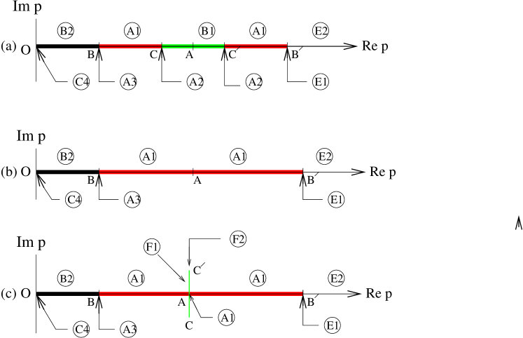
Figure 2: Schematic diagram of the spectrum for the standing wave solution with $N=2,~{}\delta=\pi$, for an appropriately chosen $\omega$ and for three values of $\gamma$, respectively less than, equal to, and greater than the critical value, see text; dispositions of the Floquet multipliers for the different band segments are indicated in accordance with notation in fig. 1

.

As mentioned above, Fig. 2(a,b,c), depicts schematically the detailed structure of the band for three different values of $\gamma$, namely $\gamma=\gamma_{c}-\epsilon,$ $\gamma=\gamma_{c},$ $\gamma=\gamma_{c}+\epsilon$ respectively, where $\epsilon$ is sufficiently small. The dispositions of the Floquet multipliers in the different segments of the band are indicated in each case, in accordance with the notation of fig. 1 and fig. 3 (see below). One observes that at the critical value $\gamma=\gamma_{c}$ (fig. 2(b)) the segment CC’ of fig. 2(a) shrinks to the point $A$, i.e., the two transition points C,C’ corresponding to the solutions of condition I (configuration A2 of fig. 1) collide and, for $\gamma>\gamma_{c}$ (fig. 2(c)), these move off the real line into the complex plane. The spectrum thereby includes the segment CAC’ stretching into the complex plane, and the standing wave solution becomes unstable. At the point $A$ (fig. 2(c)), the disposition of multipliers is like A1 of fig. 1, i.e, both pairs reside on the unit circle. For any $p$ in the interior of the segments AC or AC’, the disposition of multipliers is like that marked F1 in fig. 3 where one pair continues to reside on the unit circle while the other pair moves off into the complex $\lambda$-plane (the stretches AC and AC’ in fig. 2(c) are not actually straight, but curved lines). At the edges C, C’ (fig. 2(c)), condition I is again satisfied (but with $T,~{}P$ lying in a region of the $P$-$T$ plane different from the one corresponding to C or C’ in fig. 2(a)), and the disposition of multipliers is like F2 in Fig. 3.

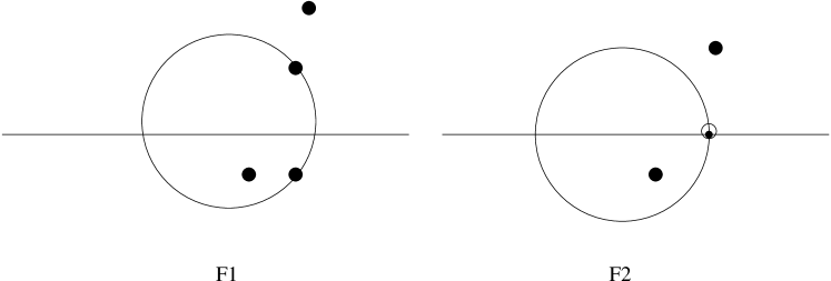
Figure 3: Schematic diagram of a pair of possible dispositions of Floquet multipliers for a complex $p$.

Let us consider, for $\gamma=\gamma_{c}-\epsilon$, two points in the spectrum, one with $p=p_{1}-\delta$ (slightly left of C) and the other with $p=p_{2}+\delta$ (slightly right of C’) where $\delta$ is small. For each of these points there are two pairs of multipliers on the unit circle, of which one pair is close to $+1$. For $p=p_{1}-\delta$, we denote the eigenmodes of the pair located away from $+1$ as $\chi_{1},~{}\chi_{2}$ (they are complex conjugate to one another), and the remaining two eigenmodes ( for multipliers close to $+1$) as $\chi_{3},~{}\chi_{4}$ (again mutually complex conjugate). Similarly, for $p=p_{2}+\delta$ we denote the corresponding eigenmodes as $\chi^{\prime}_{1}$, $\chi^{\prime}_{2}$, $\chi^{\prime}_{3}$ and $\chi^{\prime}_{4}$. All the eigenmodes have the general form

$$\left(\begin{array}[]{l}a_{2k}\\ a_{2k-1}\\ {b^{*}}_{2k}\\ {b^{*}}_{2k-1}\end{array}\right)=e^{ik\phi}\left(\begin{array}[]{l}\alpha\\ \beta\\ \gamma\\ \delta\end{array}\right),$$ (48)

for which the Krein signature is

$$\sigma=sign(|\alpha|^{2}+|\beta|^{2}-|\gamma|^{2}-|\delta|^{2}).$$ (49)

In the present case all the eigenmodes can be explicitly obtained and one finds

$$K(p_{2}+\delta;\chi^{\prime}_{1})=K(p_{2}+\delta;\chi^{\prime}_{2})=K(p_{1}-\delta;\chi_{1})=K(p_{1}-\delta;\chi_{2})=~{}-$$ (50a)

$$K(p_{2}+\delta;\chi^{\prime}_{3})=K(p_{2}+\delta;\chi^{\prime}_{4})=-K(p_{1}-\delta;\chi_{3})=-K(p_{1}-\delta;\chi_{4})=~{}-.$$ (50b)

Thus, the Krein signatures associated with the eigenfrequencies $p_{1}-\delta$ and $p_{2}+\delta$ are respectively

$$K(p_{1}-\delta)=0,$$ (51a)

$$K(p_{2}+\delta)=-.$$ (51b)

These are also the signatures for all $p$ in the interior of the segments C’B’ and BC respectively. As regards the signatures for the transition points C and C’ $(\delta=0)$ the situation is slightly different. In case of C ($p=p_{1}$), for instance, there are again two eigenmodes $\chi_{1},~{}\chi_{2}$ (complex conjugate of each other) of the form (48). For the multiplier $+1,$ one eigenmode ($\chi_{3}$, say) is again of the form (48) with $(\phi=0)$, while there exits another eigenmode $\chi_{4}$ that diverges linearly with site index $n$. The signature for $\chi_{4}$ is not well defined while that for $\chi_{1},~{}\chi_{2},~{}\chi_{3}$ are as in (50a,50b). Similar statements apply for the transition point C’ $(p=p_{2})$.

At the collision ($\gamma=\gamma_{c}$, fig. 2(b)) where C and C’ coalesce at A, the Krein signatures for any eigenfrequency in the interior of AB’ and BA are again as in (51a,51b) respectively. As regards the point A $(p=\bar{p},~{}\gamma=\gamma_{c})$ the signature for the two eigenmodes $\chi_{1},~{}\chi_{2}$ corresponding to the pair of multipliers located away from $+1$ is again ‘$-$’, while that for $\chi_{3}$ is $\sigma=0$. The other eigenmode $\chi_{4}$ for the multiplier $+1$ again diverges linearly; however, now its signature is well defined and one finds that the reduced energy restricted to the subspace spanned by $\chi_{3},~{}\chi_{4}$ is an indefinite quadratic form, so that one has, for $\gamma=\gamma_{c},$

$$K(\bar{p})=0.$$ (51c)

Summarising, we observe that for each of the colliding transition points C, C’ there exits a relevant Krein signature corresponding to $\chi_{3},~{}\chi^{\prime}_{3}$ respectively which are opposite and, at the collision, this relevant signature reduces to zero. Another way of characterising the collision is by referring to the Krein signatures for eigenfrequencies belonging to the interiors of the segments BC and B’C’ respectively. As seen from (50a, 50b), these are respectively $0$ and ${}^{\prime}-^{\prime}$. In other words, an open set of eigenfrequencies with signature $\sigma=0$ is embedded within the spectrum both before and at the collision (see ref14 ). On the other side of the collision ($\gamma>\gamma_{c}$, fig. 2(c)), the Krein signatures for eigenfrequencies in the interiors of BA, AB’ remain the same (i.e., $0$ and ${}^{\prime}-^{\prime}$ respectively), while that for the entire complex segment CAC’ one has $\sigma=0$.

Figure 4: Numerical integration of (1a), (1b) to exhibit stability of $N=2,~{}\delta=\pi$, SW solution ($\gamma=5.9765$, slightly below the critical value) starting from the profile (as function of lattice site index $n$) at (a) $t=0$ up to $\tau=5000T$ (the new profile coincides with (a)); (b) corresponds to $\tau+\frac{T}{8}$, and $\tau+\frac{7T}{8}$, (c) to $\tau+\frac{3T}{8}$, and $\tau+\frac{5T}{8}$, and (d) to $\tau+\frac{4T}{8}$.

Figure 5: Numerical integration as in fig. 4, but with $\gamma=5.9767$, slightly above the critical value, where the profile obtained for $\tau=1500T$ is shown; it differs markedly from the breather profile, similar to (a) in fig. 4, at $t=0$.

We thus have a complete description, both in terms of Floquet multipliers and Krein signatures, of the band structure and of the collision causing the onset of instability. As mentioned earlier, for every fixed $\lambda$ (and hence $\omega=-\lambda-\frac{1}{\lambda})$ there exits a critical value of $\gamma$ namely $\gamma=\gamma_{c}(\omega)=-2\omega-\frac{\omega^{3}}{16}$ such that, as $\gamma$ crosses $\gamma_{c}$ from below, the SW breather becomes unstable. We show in fig. 4, fig. 5 this loss in stabilty for $\lambda=0.5~{}(\omega=-2.5,~{}\gamma_{c}~{}\approx 5.9766)$ where we display the SW profile (eq.(2a), (12a)-(12e)), at $t=0$ as also the profile obtained by numerical integration of (1a), (1b) up to a time $\tau$ (say, see captions) for two values of $\gamma,$ one just below and the other just above $\gamma_{c}.$ One observes in these figures that the profile remains remarkably stable in fig. 4 for $\tau$ as large as $5000T$, while in fig. 5, the profile quickly breaks up even at $\tau=1500T$ ($T=$ breather time period). For each fixed value of $\lambda$ $(0<\lambda<1;~{}\omega<-2)$ the SW remains stable for a window of $\gamma$-values given by $\gamma_{1}(\lambda)<\gamma<\gamma_{c}(\lambda)$. As $\lambda$ is made to increase from $0$ to $1$ the width of the window decreases, i.e., for decreasing breather frequency, the onset of instability occurs at progressively lower values of the strength of nonlinearity $\gamma$ (fig. 6).

Figure 6: Window of stability of the $N=2,\delta=\pi$ breather; the curve with the full line corresponds to the threshold value ($\gamma_{1}(\lambda)$) of $\gamma$ below which the SW solution does not exist, while the dotted curve corresponds to the stability border; for any fixed $\lambda$, the vertical distance between the two curves depicts the $\gamma$-window of stability of the SW solution.

It is interesting to compare, for the sake of completeness, a different type of collision of eigenfrequencies, namely one where the collision does not result in the appearance of complex frequencies. Consider, for instance, $\omega=\omega_{0}=-3$ and $\gamma=\gamma_{0}=\frac{23}{3}$. With these values of $\omega$ and $\gamma$ (43a), (43b) give $z_{1}=z_{3}=9.$ $i.e.,~{}p=\pm 3$. Fig. 7(a,b,c) shows schematically the eigenfrequency spectrum for $\omega=\omega_{0}=-3,$ and for $\gamma=\gamma_{0}-\epsilon,~{}\gamma=\gamma_{0},~{}\gamma=\gamma_{0}+\epsilon$ respectively, where $\epsilon$ is sufficiently small.

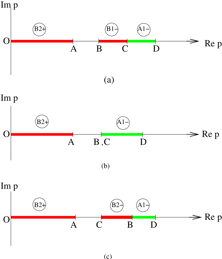
Figure 7: Schematic diagram of spectrum for $N=2,\delta=\pi$, SW solution similar to fig. 2, but now with $\omega=-3$, and three values of $\gamma$, respectively less than, equal to, and greater than $\frac{23}{3}$.

The spectrum now consists of two bands, and the various parts of the spectrum marked by transition points and band-edges have once again been marked with labels indicating the respective dispositions of Floquet multipliers in accordance with notation of fig. 1. In fig. 7(a), for instance ($\gamma=\frac{23}{3}-\epsilon$), one band extends from O($\omega=0$) to A ($\omega=\sqrt{z_{2}}$, refer to eqns.(43a)-(43c)), with only one pair of multipliers residing on the unit circle for each $p$ within this band (disposition B2 in fig.1) and the Krein signature for such a $p$ is found to be ‘$+$’. We have thus labelled the band ‘$B2+$’. The spectrum for $\omega=-3$, $\gamma=\frac{23}{3}-\epsilon$ contains a second band extending from B ($p=-\omega=\sqrt{z_{3}}$) to D($p=\sqrt{z_{4}}$) through C ($p=\sqrt{z_{1}}$), the latter being a transition point satisfying (32a). For small $\epsilon$, the width of the segment BC is small and it is labelled ‘B1-’ to denote that the disposition of the Floquet multipliers for any $p$ in the interior of the segment is B1 (fig. 1), and the Krein signature is ‘$-$’. In a similar manner, the segment CD receives the label ‘A1-’.

As $\epsilon\rightarrow 0$ i.e., $\gamma$ approaches the value $\frac{23}{3}$ from below (note that this value is less than $\gamma_{c}=7.6875,$ the critical value corresponding to $\omega=-3$ at which one has the collision $z_{1}=z_{2}$) there occurs a collision between B and C, but now the two signatures involved are the same and there does not appear complex eigenfrequencies as a result of the collision, as seen in fig. 7(b,c). We observe from fig. 7(c) that the points B, C just pass through each other, and now the eigenfrequencies $\sqrt{z_{1}},~{}\sqrt{z_{2}}$ form the band-edges.

Observe that, for $\omega=-3,$ the critical collision, leading to instability occurs for $\gamma=\gamma_{c}=7.6875,$ when in fig. 7(c), the band-edges A and C approach each other. As seen from this figure, the Krein signatures involved are now opposite, and the spectrum acquires a complex part as $\gamma$ crosses $\gamma_{c}$ from below.

In summary, we have obtained the detailed band structure for $N=2,~{}\delta=\pi$, and have characterised the various bands and band segments in terms of the Floquet multipliers and Krein signatures, and have distinguished between two types of collisions in terms of the Krein signatures of the colliding bands or segments.

5.2 Band Structure: N=3, $\delta=\pi$

As another example of a collision of intraband transition points, we consider commensurate SW solutions with $N=3,$ $\delta=\pi$ (solutions with $N=3,~{}\delta=0$ are again intrinsically unstable) given by (13a)-(13e), where explicit formulae can once again be worked out. Using the notation (42) , we now have:

$$T=(-5\omega+\frac{2}{1-\omega}-\gamma)z-(1-\omega)^{2}(\omega+2)-(\omega^{2}-1)\gamma,$$ (52a)

$$P=-z^{3}+(2\omega^{2}+8-\frac{2(1+\gamma)}{1-\omega}){z^{2}}+(-\omega^{4}+\frac{4\omega^{3}}{1-\omega}-9+2\gamma\frac{\omega^{2}+\omega+2}{1-\omega})z+$$

$$(2(\omega^{3}-3\omega+1)+2\gamma(\omega^{2}-1)).~{}~{}~{}~{}~{}~{}~{}~{}~{}~{}~{}~{}$$ (52b)

We now have, in general, three eigenfrequencies (we once again restrict to $Re(p)\geq 0$) satisfying condition I (eq. (32a)), and three others satisfying condition II (eq.(32b)), of which one is the trivial solution $p=0$, while the number of eigenfrequencies satisfying condition III depends on $\gamma,~{}\omega.$ We choose, for the sake of concreteness, $\lambda=0.5$ $(\omega=-2.5)$. Then two of the solutions to (32a) undergo a collision for $\gamma=\gamma_{c}=4.75585$ at $p=1.5750.$ We show schematically in fig. 8(a,b,c) the detailed band structures for three values of $\gamma,$ namely $\gamma_{c}-\epsilon$, $\gamma_{c}$, $\gamma_{c}+\epsilon$ respectively, where $(\epsilon>0)$ is small.

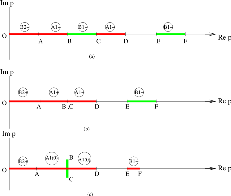
Figure 8: Schematic diagram, similar to fig. 2 and fig. 7, of the spectrum for the $N=3,\delta=\pi$ SW solution, with $\omega=-2.5$, and three values of $\gamma$, resp. smaller than, equal to, and larger than the critical value (see text).

For each of these three values of $\gamma,$ we have two bands separated by a band gap, together with a number of transition points within one of the bands. As in fig. 7 we mark each of the band segments with a label indicating the disposition of Floquet multipliers as also the Krein signature characterising that segment. In fig. 8(a,b,c) the points B, C, E correspond to condition I, while O, A, F correspond to condition II, and D corresponds to condition III. The stretch from D to E is a band gap. One observes that, at $\gamma=\gamma_{c},$ the transition points B and C within the first band collide and then stretch out into the complex plane (the segment from B to C in the complex plane in fig. 8(c) is not actually straight but is slightly curved). The label in the segment from A to D in fig. 8(c) is meant to imply that the Krein signature for any $p$ within this segment is $0$ (i.e., the reduced energy is an indefinite quadratic form on the space spanned by the eigenmodes) while the disposition of the Floquet multipliers is similar to A1 in fig. 1. We note from fig. 8(b) that the two colliding segments bear opposite Krein signatures, as a result of which they stretch out into the complex plane on the other side of the collision.

Figures 9, 10 show the results of numerical integration of an initial standing wave profile with $\lambda=0.5$, and with $\gamma=$4.75580$(<\gamma_{c})$ and $\gamma$=4.75590$(>\gamma_{c})$ respectively, where we find that the SW solution indeed gets destabilised as $\gamma$ crosses $\gamma_{c}$ from below.

Figure 9: Numerical integration of SW solution for $N=3,~{}\delta=\pi$, with $\lambda=.5$, $\gamma=4.75580$ (slightly less than $\gamma_{c}$); for explanation, see caption to fig. 4.

Figure 10: Numerical integration of SW solution for $N=3,~{}\delta=\pi$, with $\lambda=.5$, $\gamma=4.75590$ (slightly greater than $\gamma_{c}$); for explanation, see caption to fig. 5.

Fig. 11 depicts the region of stability of the standing wave solution under consideration in the $\gamma-\lambda$ parameter plane, where we once again find that, for decreasing breather frequency, the SW gets destabilised at progressively lower values of the non-linearity parameter $\gamma.$

Figure 11: Stability window for the $N=3,\delta=\pi$, SW solution; for explanation see caption to fig. 6

In conclusion, we observe that, away from the linear and the anti-continuous limits, there exist dynamically stable commensurate standing wave solutions in our DNLS-like model, in contrast to DNLS breathers close to the above two limits. The frequency spectrum and eigenmodes of the linearised systems around these SW solutions present interesting features that can be described in terms of the dispositions of Floquet multipliers as also the Krein signatures associated with the various segments of the band spectrum. The onset of instability occurs not necessarily through collisions of band-edges, but also through collisions of intra-band transition points.

In a future communication, we shall study exact commensurate and incommensurate SW solutions in a piecewise linear NDKG model and look into their stability problem, with special reference to incommensurate SW solutions. The possibility of multibreaher solutions involving an infinite array of breathers with random spatial distribution will also be investigated in these exactly solvable models.

References

- (1) G. Iooss, and K. Kirchgassner, Travelling waves in a chain of coupled non-linear oscillators, Comm. Math. Phys., 211 (2000) 439-464.
- (2) G. Ioss Travelling waves in the Fermi-Pasta-Ulam lattice, Nonlinearity, 13 (2000) 849-866.
- (3) A. M. Morgante, M. Johansson, G. Kopidkas, S. Aubry, Standing wave instabilities in a chain of non-linear coupled oscillators, Physica D, 162 (2002) 53-94.
- (4) A. M. Morgante, M. Johansson, G. Kopidkas, S. Aubry, Oscillatory instabilities of standing waves in one-dimensional non-linear lattices, Phys. Rev. Lett, 85 (2000) 550-553.
- (5) V. I. Arnold, and A. Avez, Ergodic Problems in Classical Mechanics, Benjamin, N.Y. (1968).
- (6) T. J. Bridges, Bifurcation of periodic solutions near a collision of eigenvalues of opposite signatures, Math. Proc. Camb. Phil. Soc. 108 (1990) 575-601.
- (7) T. Kapitula, P. G. Kevrikidis, and B. Sandstede, Counting eigenvalues via the Krein signature in infinite-dimensional Hamiltonian systems, Physica D, 195 (2004) 263-282.
- (8) J. Van der Meer, The Hamiltonian Hopf Bifurcation, Lect. note in Mathematics, v 116, Springer, Berlin (1985).
- (9) T. J. Bridges, Stability of periodic solutions near a collision of eigenvalues of opposite signatures, Math. Proc. Camb. Phil. Soc. 109 (1991) 375-403.
- (10) A. Lahiri, and M. Sinha Roy, The Hamiltonian Hopf bifurcation, an elementary perturbative approach, Int. J. Non-lin. Mech., 36 (2001) 787-802.
- (11) A. Lahiri, S. Panda, and T. K. Roy, Discrete breathers: exact solutions in piecewise linear models, Phys. Rev. Lett., 84 (2000) 3570-3573.
- (12) A. Lahiri, S. Panda, and T. K. Roy, Breathers in a discrete non-linear Schrödinger-type model: exact stability results, Phys. Rev. E, 66 (2002) 056603.
- (13) R. S. MacKay, Stability of equilibria in Hamiltonian systems, in R. S. MacKay and J. Meiss (eds), Hamiltonian Dynamical Systems, p 137-153, Adam Hilger, (1987).
- (14) M. Grillakis, Analysis of the linearisation around a critical point of an infinite dimensional Hamiltonian system, Comm. Pure Appl. Math, 43 (1990) 299-333.