An integrable generalization of the Toda law
to the square lattice

Abstract

We generalize the Toda lattice (or Toda chain) equation to the square lattice; i.e., we construct an integrable nonlinear equation, for a scalar field taking values on the square lattice and depending on a continuous (time) variable, characterized by an exponential law of interaction in both discrete directions of the square lattice. We construct the Darboux-Backlünd transformations for such lattice, and the corresponding formulas describing their superposition. We finally use these Darboux-Backlünd transformations to generate examples of explicit solutions of exponential and rational type. The exponential solutions describe the evolution of one and two smooth two-dimensional shock waves on the square lattice.

1 Introduction

The Toda lattice [1, 2, 3]

$$\frac{d^{2}Q_{m}}{dt^{2}}=\Delta_{m}e^{\Delta_{m}Q_{m-1}},$$ (1)

where $\Delta_{m}f_{m}=f_{m+1}-f_{m}$ is the difference operator and $Q=Q_{m}(t)$ is a dynamical function on a one dimensional lattice ($m\in{\mathbb{Z}}$), is one of the most famous integrable nonlinear lattice equations. It describes the dynamics of a one - dimensional physical lattice whose masses are subjected to an interaction potential of exponential type. The infinite, finite and periodic Toda lattice (1), as well as its numerous extensions [4, 5, 6, 7, 8, 9, 10, 11, 12], have applications in various other physical and mathematical contexts [13, 14, 15, 16, 17, 18, 19].

In this paper we introduce the following integrable generalization of the Toda law (1) (i.e., the law characterized by an exponential interaction between nearest neighbours) to a 2-dimensional lattice:

$$\begin{array}[]{l}C_{m,n}\frac{d}{dt}\!\left(\!\frac{1}{C_{m,n}}\!\frac{dQ_{m,n}}{dt}\!\right)\!=\!\Delta_{m}\!\left(\!C_{m,n}\!C_{m-1,n}e^{\Delta_{m}Q_{m\!-\!1,\!n}}\right)\!+\!\Delta_{n}\!\left(\!C_{m,n}\!C_{m,\!n\!-\!1}e^{\Delta_{n}\!Q_{m,n\!-\!1}}\right),\\ {}{}\\ \frac{C_{m+1,n+1}}{C_{m,n}}=e^{-\Delta_{m}\Delta_{n}Q_{m,n}},\end{array}$$ (5)

where $Q=Q_{m,n}(t)$ and $C=C_{m,n}(t)$ are dynamical functions on the square lattice ($(m,n)\in{\mathbb{Z}}^{2}$) and $\Delta_{m}f_{m,n}=f_{m+1,n}-f_{m,n},~{}~{}~{}\Delta_{n}f_{m,n}=f_{m,n+1}-f_{m,n}$ are the difference operators in the $m$ and $n$ directions.

Starting with the linear 5-point scheme (16) [20], in §2 we construct a Lax pair for eq. (5); in §3 we construct the Darboux-Bäcklund Transformations (DBTs) for this 2D Toda lattice, and the corresponding formulas describing the superposition of such DBTs; in §4 we use these transformations to construct explicit solutions of exponential and rational type of the 2+1 dimensional Toda lattice (5).

We remark that, in the literature related to integrable systems, there exist already three 2+1 dimensional generalizations of the Toda lattice (1). The first one is obtained replacing the second derivative $d^{2}/dt^{2}$ in (1) by the hyperbolic operator $\partial^{2}/\partial x\partial y$ [8] (see also [21, 22]), or by the elliptic operator $\partial^{2}/\partial z\partial\bar{z}$. In this equation, therefore, the scalar field $Q$ depends on two continuous variables $x,y$ and on one discrete variable $m$: $Q_{m}(x,y)$. The second generalization [5] can be viewed as a variant of the first, in which one of the two continuous variables, say $x$, is suitably discretized. The third generalization [6, 7] is obtained discretizing both $x$ and $y$ variables. In the generalization (5) we propose in this paper, instead, the scalar field $Q$ depends on the continuous time variable $t$, through the Sturm-Liouville operator in the left hand side of (5), and on the two discrete indeces $(m,n)\in{\mathbb{Z}}^{2}$ of the square lattice ($Q=Q_{m,n}(t)$), through the exponential law of interaction between nearest neighbours in both $m$ and $n$ directions.

We remark that a 2+1 dimensional generalization of the Volterra system on the square lattice has recently appeared [23].

2 The 2D generalization of the Toda lattice

The Lax pair (zero curvature representation) for the Toda lattice can be written in the following form [24],[25]:

$$\begin{array}[]{l}\frac{\Gamma_{m}}{\Gamma_{m+1}}\phi_{m+1}+\frac{\Gamma_{m-1}}{\Gamma_{m}}\phi_{m-1}-F_{m}\phi_{m}=\lambda\phi_{m},\\ \frac{d\phi_{m}}{dt}=\frac{\Gamma_{m}}{\Gamma_{m+1}}\phi_{m+1}-\frac{\Gamma_{m-1}}{\Gamma_{m}}\phi_{m-1},\end{array}$$ (8)

where $\lambda$ is the constant eigenvalue of the self-adjoint 3-point scheme (8a), $\Gamma_{m}(t),F_{m}(t)$ are dynamical functions on the lattice, the eigenfunction $\phi_{m}(t,\lambda)$ solves simultaneously the Lax pair (8), and the Toda field $Q$ is related to $\Gamma,F$ in the following way

$$F_{m}=-\frac{dQ_{m}}{dt},~{}~{}~{}~{}~{}\Gamma_{m}=e^{-\frac{Q_{m}}{2}}.$$ (9)

A key progress towards the generalization of the Toda law (1) to a 2-dimensional lattice has been recently made in [20]; in that paper, devoted to the investigation of discretizations of elliptic operators on 2D lattices admitting Darboux transformations (DTs), the following results were, in particular, established.

• The linear and self-adjoint 5-point scheme on the star of the square lattice:

  $$\begin{array}[]{l}{\mathcal{L}}_{5}\tilde{\psi}_{m,n}:=a_{m,n}\tilde{\psi}_{m+1,n}+a_{m-1,n}\tilde{\psi}_{m-1,n}+\\ b_{m,n}\tilde{\psi}_{m,n+1}+b_{m,n-1}\tilde{\psi}_{m,n-1}-f_{m,n}\tilde{\psi}_{m,n}=0,\end{array}$$ (12)

  a natural discretization of the self-adjoint elliptic (if $AB>0$) operator

  $$(A\Psi_{x})_{x}+(B\Psi_{y})_{y}={\mathcal{D}}\Psi$$ (13)

  in canonical form, admits DTs.

• The 5-point scheme (12) admits a distinguished gauge equivalent form:

  $$\begin{array}[]{l}{\mathcal{L}}_{SchInt}\psi_{m,n}:=\frac{\Gamma_{m,n}}{\Gamma_{m+1,n}}\!\psi_{m+1,n}\!+\!\frac{\Gamma_{m-1,n}}{\Gamma_{m,n}}\!\psi_{m-1,n}\!+\\ \frac{\Gamma_{m,n}}{\Gamma_{m,n+1}}\!\psi_{m,n+1}\!+\!\frac{\Gamma_{m,n-1}}{\Gamma_{m,n}}\!\psi_{m,n-1}\!-\!F_{m,n}\!\psi_{m,n}=0,\end{array}$$ (16)

  obtained from (12) via the following gauge transformation:

  $${\mathcal{L}}_{SchInt}=\frac{g_{m,n}}{\Gamma_{m,n}}{\mathcal{L}}_{5}\frac{g_{m,n}}{\Gamma_{m,n}},$$ (17)

  with $F_{m,n}=f_{m,n}(g^{2}_{m,n}/\Gamma^{2}_{m,n})$, where $g$ and $\Gamma$ are defined by:

  $$a_{m,n}g_{m+1,n}=b_{m,n}g_{m+1,n},~{}~{}~{}\Gamma_{m,n}=\sqrt{a_{m,n}g_{m,n}g_{m+1,n}}=\sqrt{b_{m,n}g_{m,n}g_{m,n+1}}.$$ (18)

The linear problem (16), a natural 2D generalization of the linear problem (8a), satisfies the following basic properties: i) it possesses DTs (inherited from the DTs of (12)); ii) it reduces, in the natural continuous limit, to the 2D Schrödinger equation:

$$\psi_{xx}+\psi_{yy}+u(x,y)\psi=0.$$ (19)

For these two reasons the self-adjoint 5-point scheme (16) was identified in [20] as a proper ”integrable” discretization of the 2D Schrödinger equation, a good starting point in the search for integrable discretisations of the nonlinear symmetries associated with the spectral problem (19) and in the search for an integrable generalization of the Toda equation to a square lattice.

The 2 dimensional generalization of the Lax pair (8) proposed in this paper is indeed based on the linear problem (16), and reads

$$\begin{array}[]{l}\frac{\Gamma_{m,n}}{\Gamma_{m+1,n}}\psi_{m+1,n}+\frac{\Gamma_{m-1,n}}{\Gamma_{m,n}}\psi_{m-1,n}+\frac{\Gamma_{m,n}}{\Gamma_{m,n+1}}\psi_{m,n+1}+\frac{\Gamma_{m,n-1}}{\Gamma_{m,n}}\psi_{m,n-1}=F_{m,n}\psi_{m,n},\\ {}{}\\ \frac{d\psi_{m,n}}{dt}=\frac{C_{m,n}}{2}\left[\frac{\Gamma_{m,n}}{\Gamma_{m+1,n}}\psi_{m+1,n}-\frac{\Gamma_{m-1,n}}{\Gamma_{m,n}}\psi_{m-1,n}+\frac{\Gamma_{m,n}}{\Gamma_{m,n+1}}\psi_{m,n+1}-\frac{\Gamma_{m,n-1}}{\Gamma_{m,n}}\psi_{m,n-1}\right].\end{array}$$ (23)

It is easy to verify that this system of linear equations for the eigenfunction $\psi_{m,n}(t)$ is compatible iff the coefficients $\Gamma,F,C$ satisfy the following nonlinear equations:

$$\begin{array}[]{l}\frac{dF_{m,n}}{dt}\!=\!C_{m+1,n}\!\left(\frac{\Gamma_{m,n}}{\Gamma_{m+1,n}}\right)^{2}\!\!\!\!-\!C_{m-1,n}\!\left(\frac{\Gamma_{m-1,n}}{\Gamma_{m,n}}\right)^{2}\!\!\!+\!C_{m,n+1}\!\left(\frac{\Gamma_{m,n}}{\Gamma_{m,n+1}}\right)^{2}\!\!\!-\!C_{m,n-1}\!\left(\frac{\Gamma_{m,n-1}}{\Gamma_{m,n}}\right)^{2}\!\!\!,\\ {}{}\\ \frac{d\Gamma_{m,n}}{dt}=\frac{1}{2}C_{m,n}F_{m,n}\Gamma_{m,n},\\ {}{}\\ \frac{C_{m+1,n+1}}{C_{m,n}}=\left(\frac{\Gamma_{m+1,n+1}\Gamma_{m,n}}{\Gamma_{m+1,n}\Gamma_{m,n+1}}\right)^{2}.\end{array}$$ (29)

Equations (29) can be conveniently rewritten as the 2+1 dimensional generalization (5) of the exponential interaction law of Toda, in terms of the scalar field $Q_{m,n}(t)$ defined by

$$F_{m,n}C_{m,n}=-\frac{dQ_{m,n}}{dt},~{}~{}~{}~{}~{}\Gamma_{m,n}=e^{-\frac{1}{2}Q_{m,n}}.$$ (30)

In the one dimensional limit in which $\psi_{m,n}(t)$ depends trivially on $n$ and the coefficients $\Gamma,F,C$ do not depend on $n$:

$$\psi_{m,n}(t)=\phi_{m}(t)(-z)^{n},~{}~{}\Gamma_{m,n}=\Gamma_{m},~{}~{}F_{m,n}=F_{m},~{}C_{m,n}=C_{m},$$ (31)

it follows from (5b) that $C$ is an arbitrary function of $t$ independent of $m$: $C_{m}(t)=C(t)$ and equation (5a) reduces to

$$\frac{1}{C(t)}\frac{d}{dt}\left(\frac{1}{C(t)}\frac{dQ_{m}}{dt}\right)=\Delta_{m}e^{\Delta_{m}Q_{m-1}}.$$ (32)

Suitably rescaling $t$ (or choosing $C(t)=1$), one finally recovers the Toda lattice (1) and its Lax pair (8), with $\lambda=z+z^{-1}$.

We first remark that the 5-point schemes (23) on the star of the square lattice are the simplest and natural generalization of the 3-point schemes (8). Therefore we expect that our Toda 2D lattice (5) be the simplest integrable generalization of (1) on the square lattice.

We also remark that the Toda 2D-lattice system (5) can be rewritten as a single equation, observing that equation (5b) is identically satisfied by the following parametrization

$$\Gamma^{2}_{m,n}=\frac{\tau_{m,n}}{\tau_{m+1,n+1}},~{}~{}~{}C_{m,n}=\frac{\tau_{m+1,n}\tau_{m,n+1}}{\tau_{m,n}\tau_{m+1,n+1}}$$ (33)

in terms of the single scalar field $\tau_{m,n}$. Then the system (5) reduces to the single equation

$$\begin{array}[]{l}W[\!\tau_{m+1,n}\!\tau_{m,n+1},W[\tau_{m+1,n+1},\!\tau_{m,n}]]\!=\!\tau^{2}_{m+1,n}\left(\tau_{m,n}\!\tau_{m,n+2}\!-\!\tau_{m+1,n+1}\!\tau_{m-1,n+1}\right)+\\ \tau^{2}_{m,n+1}\left(\tau_{m,n}\!\tau_{m+2,n}\!-\!\tau_{m+1,n+1}\!\tau_{m+1,n-1}\right),\end{array}$$ (36)

where

$$W[\alpha,\beta]:=\alpha\dot{\beta}-\dot{\alpha}\beta$$ (37)

is the usual Wronskian of the two functions $\alpha$ and $\beta$. It turns out [26] that the scalar function $\tau_{m,n}(t)$ is related to the $\tau$-function of the BKP hierarchy [27]; therefore equation (36) gives the $\tau$-function formulation of the 2+1 dimensional Toda system (5).

If the $\tau$-function depends only on $m$: $\tau_{m,n}(t)=\tau_{m}(t)$, equation (36) reduces to equation

$$\tau_{m+1}^{2}H[\tau_{m}]-\tau_{m}^{2}H[\tau_{m+1}]=0,$$ (38)

where

$$H[\tau_{m}]:=\ddot{\tau}_{m}\tau_{m}-{\dot{\tau}}^{2}_{m}+\tau_{m+1}\tau_{m-1}-\tau^{2}_{m},$$ (39)

implying that

$$H[\tau_{m}]=f(t)\tau^{2}_{m},$$ (40)

with $f(t)$ arbitrary function of $t$. By the change of variable $\tilde{\tau}_{m}(t)=\break exp(-y(t))\tau_{m}(t)$, with $\ddot{y}(t)=f(t)$, we recover the $\tau$-function formulation [4] $H[\tilde{\tau}_{m}]=0$ of the Toda lattice (1).

We finally remark that $F$ and $C$ constants and $\Gamma=e^{\frac{CF}{2}t}$ is the trivial solution of (29); correspondingly: $Q=-FCt$ blows linearly in time. Solutions which are perturbations of this solution will exhibit such a linear blow up in time, which can be removed introducing the change of variables $Q_{m,n}=P_{m,n}-FCt+\delta$. Then equation (5) becomes:

$$\begin{array}[]{l}C_{m,n}\frac{d}{dt}\!\left(\!\frac{1}{C_{m,n}}\!\left(\frac{dP_{m,n}}{dt}\!+\!FC\!\right)\!\right)\!=\!\Delta_{m}\!\left(\!C_{m,n}\!C_{m-1,n}e^{\Delta_{m}P_{m-1,n}}\right)\!+\\ +\Delta_{n}\!\left(\!C_{m,n}\!C_{m,n-1}e^{\Delta_{n}P_{m,n-1}}\right),~{}~{}~{}~{}~{}~{}~{}\frac{C_{m+1,n+1}}{C_{m,n}}=e^{-\Delta_{m}\Delta_{n}P_{m,n}}.\end{array}$$ (43)

We end this section remarking that algebro-geometric solutions of the eigenvalue problem for a generic 5-point scheme were constructed in [28].

3 Darboux-Backlünd transformations and their superposition

It is a straightforward (but long) calculation to verify that the DBTs for the 2D generalization of the Toda lattice (29), (5) read as follows:

$$\begin{array}[]{l}\Delta_{m}\left(\frac{\Gamma^{\prime}}{\Gamma}\theta\psi^{\prime}\right)_{m,n}=\frac{\Gamma_{m,n-1}}{\Gamma_{m,n}}\theta_{m,n}\theta_{m,n-1}\tilde{\Delta}_{-n}\frac{\psi_{m,n}}{\theta_{m,n}},\\ \Delta_{n}\left(\frac{\Gamma^{\prime}}{\Gamma}\theta\psi^{\prime}\right)_{m,n}=-\frac{\Gamma_{m-1,n}}{\Gamma_{m,n}}\theta_{m,n}\theta_{m,n-1}\tilde{\Delta}_{-m}\frac{\psi_{m,n}}{\theta_{m,n}},\\ \frac{d}{dt}\left(\frac{\Gamma^{\prime}}{\Gamma}\theta\psi^{\prime}\right)_{m,n}=C_{m,n}\frac{\Gamma_{m-1,n}\Gamma_{m,n-1}}{\Gamma_{m,n}^{2}}\theta_{m-1,n}\theta_{m,n-1}\left(\frac{\psi_{m-1,n}}{\theta_{m-1,n}}-\frac{\psi_{m,n-1}}{\theta_{m,n-1}}\right),\end{array}$$ (47)

$$\begin{array}[]{l}\Gamma^{\prime}\,{}^{2}_{m,n}=(\Gamma\theta)_{m-1,n-1}\frac{\Gamma_{m,n}}{\theta_{m,n}},\\ C_{m,n}^{\prime}=\frac{(\Gamma\theta)_{m-1,n}(\Gamma\theta)_{m,n-1}}{(\Gamma\theta)_{m,n}(\Gamma\theta)_{m-1,n-1}}C_{m,n},\\ F^{\prime}_{m,n}=(\Gamma\theta)_{m-1,n-1}\left[\frac{1}{(\Gamma\theta)_{m-1,n}}+\frac{1}{(\Gamma\theta)_{m,n-1}}\right]+\frac{\theta_{m,n}}{\Gamma_{m,n}}\left[\left(\frac{\Gamma}{\theta}\right)_{m-1,n}+\left(\frac{\Gamma}{\theta}\right)_{m,n-1}\right],\end{array}$$ (51)

where $\tilde{\Delta}_{-m}f_{m,n}=f_{m,n}-f_{m-1,n}$ and $\tilde{\Delta}_{-n}=f_{m,n}-f_{m,n-1}$. In these equations: $\theta_{m,n}(t)$ is a solution of the Lax pair (23), for the coefficients $\Gamma_{m,n},F_{m,n},C_{m,n}$; $\psi^{\prime}_{m,n}(t)$ in (47) is the transformed (via $\theta_{m,n}$) solution of the Lax pair (23), for the transformed (via (51)) coefficients $\Gamma^{\prime}_{m,n},F^{\prime}_{m,n},C^{\prime}_{m,n}$.

The so-called spatial part of the above DBTs was already written in [20]; the temporal part, describing the time dependence of the transformed solution $\psi^{\prime}_{m,n}(t)$ of (23), and the transformation law (51b) for the coefficient $C_{m,n}(t)$, are new results of this paper.

It is well-known [29] that it is possible to combine DBTs of a given integrable system, to construct superposition formulas and a permutability diagram of DBTs. For the 2D Toda lattice (29),(5) it is possible to prove the following result (see also [26] for the Bianchi permutability diagram of the general self-adjoint scheme on the star of the square lattice).

Consider a solution ($\Gamma_{m,n},F_{m,n},C_{m,n}$) of the 2D Toda lattice (29),(5), and let $\theta^{(1)}_{m,n}$ and $\theta^{(2)}_{m,n}$ be two independent solutions of the Lax pair (23), corresponding to the coefficients $\Gamma_{m,n},F_{m,n},C_{m,n}$. Superimposig the two DBTs (47) with respect to $\theta^{(1)}_{m,n}$ and $\theta^{(2)}_{m,n}$, one obtains the new solution ($\Gamma^{(12)}_{m,n},F^{(12)}_{m,n},C^{(12)}_{m,n}$) of the nonlinear system (29)-(5) through the following formulas:

$$\begin{array}[]{l}(\Gamma^{(12)}_{m+1,n+1})^{2}=(\Gamma_{m,n})^{2}\frac{\Sigma_{m,n}}{\Sigma_{m+1,n+1}},\\ \\ F^{(12)}_{m+1,n+1}=F_{m,n}+\frac{1}{\Sigma_{m,n+1}}\frac{\Gamma_{m-1,n}}{\Gamma_{m,n+1}}(\theta^{(1)}_{m-1,n}\theta^{(2)}_{m,n+1}-\theta^{(1)}_{m,n+1}\theta^{(2)}_{m-1,n})+\\ \\ \frac{1}{\Sigma_{m+1,n}}\frac{\Gamma_{m,n-1}}{\Gamma_{m+1,n}}(\theta^{(1)}_{m+1,n}\theta^{(2)}_{m,n-1}-\theta^{(1)}_{m,n-1}\theta^{(2)}_{m+1,n})=\\ \\ =\frac{\Sigma_{m,n}\Sigma_{m+1,n+1}}{\Sigma_{m+1,n}\Sigma_{m,n+1}}[F_{m,n}+\frac{1}{\Sigma_{m+1,n+1}}\frac{\Gamma^{2}_{m,n}}{\Gamma_{m+1,n}\Gamma_{m,n+1}}(\theta^{(1)}_{m,n+1}\theta^{(2)}_{m+1,n}-\theta^{(1)}_{m+1,n}\theta^{(2)}_{m,n+1})+\\ \\ \frac{1}{\Sigma_{m,n}}\frac{\Gamma_{m-1,n}\Gamma_{m,n-1}}{\Gamma^{2}_{m,n}}(\theta^{(1)}_{m,n-1}\theta^{(2)}_{m-1,n}-\theta^{(1)}_{m-1,n}\theta^{(2)}_{m,n-1})]\\ \\ C^{(12)}_{m+1,n+1}=\left(\frac{\Gamma_{m+1,n}\Gamma_{m,n+1}}{\Gamma_{m,n}\Gamma_{m+1,n+1}}\right)^{2}\frac{\Sigma_{m+1,n}\Sigma_{m,n+1}}{\Sigma_{m,n}\Sigma_{m+1,n+1}}C_{m+1,n+1},\end{array}$$ (52)

where the function $\Sigma_{m,n}$ is obtained integrating the first order compatible equations

$$\begin{array}[]{l}\frac{d}{dt}\Sigma_{m,n}=C_{m,n}\frac{\Gamma_{m-1,n}\Gamma_{m,n-1}}{\Gamma^{2}_{m,n}}(\theta^{(1)}_{m,n-1}\theta^{(2)}_{m-1,n}-\theta^{(1)}_{m-1,n}\theta^{(2)}_{m,n-1})\\ \Sigma_{m+1,n}-\Sigma_{m,n}=\frac{\Gamma_{m,n-1}}{\Gamma_{m,n}}(\theta^{(1)}_{m,n-1}\theta^{(2)}_{m,n}-\theta^{(1)}_{m,n}\theta^{(2)}_{m,n-1}),\\ \Sigma_{m,n+1}-\Sigma_{m,n}=\frac{\Gamma_{m-1,n}}{\Gamma_{m,n}}(\theta^{(1)}_{m,n}\theta^{(2)}_{m-1,n}-\theta^{(1)}_{m-1,n}\theta^{(2)}_{m,n}).\end{array}$$ (53)

This scheme is often used to construct the two-soliton solution knowing the one-soliton solution of the system (in this case $\theta^{(1)}_{m,n}$ and $\theta^{(2)}_{m,n}$ are the eigenfunctions of the one-soliton solution corresponding to two different sets of parameters).

4 Solutions of exponential and rational type

The existence of DBTs is considered one of the basic properties of an integrable nonlinear system. In particular, it allows one to construct iteratively solutions from simpler solutions, via an endless procedure.

In this section we show some example of explicit solutions of exponential and rational type of the 2D Toda lattice (5), obtained using the DBTs (51).

We consider as starting solution of the system (29) the trivial one, corresponding to $F,C$ constants and $\Gamma=e^{\frac{FC}{2}t}$ (for this solution $Q=-FCt$) and, correspondingly, we look for an exponential solution of the Lax pair (23):

$$\psi_{m,n}(t)=e^{\alpha m+\beta n+\omega t+\delta},$$ (54)

obtaing for the coefficients $\alpha,\beta,\omega$ the following equations:

$$\begin{array}[]{c}\cosh\alpha+\cosh\beta=\frac{F}{2},\\ \sinh\alpha+\sinh\beta=\frac{\omega}{C}.\end{array}$$ (57)

These equations can be interpreted in the following way: given the constants $F,C$, equation (57a) establishes a constraint between the “wave numbers” $\alpha$ and $\beta$; once this constraint is satisfied, equation (57b) gives the “dispersion relation” $\omega$ in terms of $\alpha$ and $\beta$.

Looking for real and non singular solutions of exponential type, in the following we restrict our analysis to the case $F,C,\alpha,\beta,\delta\in{\mathbb{R}}$, postponing the study of other possible choices to a subsequent work. Then equation (57) implies that $F\geq 4$ and that the parameters $\alpha$ and $\beta=\cosh^{-1}(\frac{F}{2}-\cosh\alpha)$ must range in the interval

$$1<\cosh\alpha,\cosh\beta\leq\frac{F}{2}-1,~{}~{}~{}F\geq 4$$ (58)

(if $F=4$, then $\alpha=\beta=0$).

We consider now the following solution of (23):

$$\begin{array}[]{l}\theta_{m,n}(t)=\cosh\Theta^{+}_{m,n}(t)+\rho\cosh\Theta^{-}_{m,n}(t),\\ \Theta^{\pm}_{m,n}(t):=\alpha m\pm\beta n+\omega^{\pm}t+\delta^{\pm},~{}~{}\omega^{\pm}:=C(\sinh\alpha\pm\sinh\beta),\end{array}$$ (61)

consisting of a suitable combination of four exponentials of the type (54), where $\alpha,\beta$ satisfy the constraint (57a), and $\rho\geq 0,~{}\delta^{\pm}\in{\mathbb{R}}$.

Applying the DBTs (51) to this basic solution, one obtains the following dressed solution of the 2D Toda lattice (29),(5):

$$\begin{array}[]{l}{{\Gamma^{\prime}}^{2}_{m,n}}=e^{-Q^{\prime}_{m,n}(t)}=\frac{\cosh\Theta^{+}_{m-1,n-1}(t)+\rho\cosh\Theta^{-}_{m-1,n-1}(t)}{\cosh\Theta^{+}_{m,n}(t)+\rho\cosh\Theta^{-}_{m,n}(t)}e^{FCt},\\ C^{\prime}_{m,n}(t)=\frac{[\cosh\Theta^{+}_{m-1,n}(t)+\rho\cosh\Theta^{-}_{m-1,n}(t)][\cosh\Theta^{+}_{m,n-1}(t)+\rho\cosh\Theta^{-}_{m,n-1}(t)]}{[\cosh\Theta^{+}_{m,n}(t)+\rho\cosh\Theta^{-}_{m,n}(t)][\cosh\Theta^{+}_{m-1,n-1}(t)+\rho\cosh\Theta^{-}_{m-1,n-1}(t)]}C.\end{array}$$ (64)

This solution exhibits, depending on the value of $\rho\geq 0$, the following different features.

i) If $\rho=0$, we have the simplified expression:

$$\begin{array}[]{l}{{\Gamma^{\prime}}^{2}_{m,n}}=e^{-Q^{\prime}_{m,n}(t)}=\frac{\cosh\Theta^{+}_{m-1,n-1}(t)}{\cosh\Theta^{+}_{m,n}(t)}e^{FCt},\\ C^{\prime}_{m,n}(t)=\frac{[\cosh\Theta^{+}_{m-1,n}(t)][\cosh\Theta^{+}_{m,n-1}(t)]}{[\cosh\Theta^{+}_{m,n}(t)][\cosh\Theta^{+}_{m-1,n-1}(t)]}C.\end{array}$$ (67)

This solution describes a smooth $2D$-shock wave (a kink); the shock front is the phase (straight) line $\Theta^{+}=const$, forming with the $m$ - axis the angle $-\theta$, with $\theta=tan^{-1}\frac{\alpha}{\beta}$. This shock wave propagates with speed v${}^{+}=-\frac{\omega^{+}}{2}\sin(2\theta)(1/\beta,1/\alpha)$. The values of $Q^{\prime}_{m,n}+FCt$ ahead and behind the shock front are respectively $-(\alpha+\beta)$ and $\alpha+\beta$; then the shock strength is $2(\alpha+\beta)$ (see Fig. 1).

ii) If $\rho$ is a finite positive number, the solution describes two smooth $2D$-shock waves with the following features. The phase (straight) lines $\Theta^{\pm}=const$ form with the $m$ - axis the angles $\mp\theta$; they travel with speeds v${}^{\pm}=-\frac{\omega^{\pm}}{2}\sin(2\theta)(1/\beta,\pm 1/\alpha)$ and, consequently, their intersection point $P$ travels with constant speed v${}_{P}=-C(\frac{\sinh\alpha}{\alpha},\frac{\sinh\beta}{\beta})$. In this situation the two shock fronts do not coincide, as before, with the phase lines; they are now parallel to the $m$ and $n$ axes and intersect in P, dividing the $(m,n)$ plane in the usual 4 quadrants. The values of $Q_{m,n}+FCt$ in the first, second, third and fourth quadrants are, respectively, $\alpha+\beta$, $-\alpha+\beta$, $-(\alpha+\beta)$, and $\alpha-\beta$ (see Fig. 2).

iii) If $\rho$ is a very small positive parameter: $0<\rho<<1$, the previous two regimes combine in the following way. In the finite $(m,n)$ plane (or, more precisely, in an inner region of the order $O(\ln(1/\rho)))$, the term $\rho\cosh\Theta^{-}$ is negligeable and the expression (67) is a good approximation of the solution, which then describes the single transversal shock wave of the regime i). In the outer region, that term is not negligeable anymore and the regime ii) becomes dominant. Both ends of the transversal shock front bifurcate into two semilines parallel to the $m$ and $n$ axes (see Fig.s 3 and 4). One could actually say that the regime iii) is the generic one; but, for $\rho=O(1)$, the inner region is not visible, since it is smaller than a single elementary square of the square lattice $(m,n)$. The inner region is visible if it contains at least one elementary square of the lattice. If the spacing of the square lattice is $1$, a rough extimate for this condition is that $0<\rho<min(1/(|\alpha|e),1/(|\beta|e))$, where $e$ is the Neper constant.

The possible existence of web-like structures in the inner region, typical of 2+1 dimensional soliton models [30], will be explored in a subsequent work.

Starting with the trivial solution $F=4,~{}C$ constant ($\Rightarrow~{}\Gamma=e^{4Ct}$) of the system (29), it is also possible to construct rational solutions. It is straightforward to verify, for instance, that

$$\theta_{m,n}(t):=mn+(Ct+a)m+(Ct+b)n+C^{2}t^{2}+C(a+b)t+d$$ (68)

is a polynomial solution of the system (23), where $a,b,d$ are arbitrary constant coefficients. Substituting it into the DBTs (51), one obtains a (singular) rational solution of the 2D-Toda lattice. We remark that this solution could have been derived directly from the solution (64) for a suitable choice of its free parameters.

Acknowledgments This work was supported by the cultural and scientific agreements between the University of Roma “La Sapienza” and the Universities of Warsaw and Olsztyn. It was partially supported by KBN grant 2 P03B 126 22.

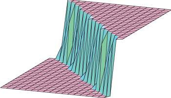
Figure 1: If $\rho=0$ and $\alpha,\beta\in{\mathbb{R}}~{}(F>4)$, the solution $Q_{m,n}+FCt$ in (64) describes a smooth 2D-shock wave propagating with velocity v${}^{+}=-\frac{\omega^{+}}{2}\sin(2\theta)(1/\beta,1/\alpha)$. The shock front is a straight line forming the angle $-\theta$, $\theta=tan^{-1}\frac{\alpha}{\beta}$ with the $m$- axis. In this figure: $\alpha=5,~{}\beta=4~{}(F=101),~{}\delta^{\pm}=1,~{}C=1,~{}\rho=0$

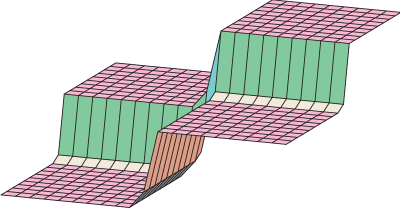
Figure 2: For $\alpha,\beta\in{\mathbb{R}}~{}(F>4)$ and $\rho=O(1)$, the solution $Q_{m,n}+FCt$ in (64) describes two shock waves with fronts parallel to the $m$ and $n$ axes. The intersection point $P$ of these two fronts travels with velocity v${}_{P}=-C(\frac{\sinh\alpha}{\alpha},\frac{\sinh\beta}{\beta})$. In this figure: $\alpha=5,~{}\beta=4~{}(F=101),~{}\delta^{\pm}=1,~{}C=1,~{}\rho=1$

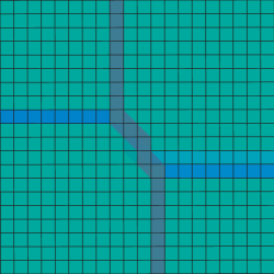
Figure 3: A view from the top of the solution for $\rho=10^{-7}$. In the central (finite) region, the single shock prevails; this single shock matches with the two orthogonal shocks, which prevail instead in the outer region. In this figure: $\alpha=5,~{}\beta=4~{}(F=101),~{}\delta^{\pm}=1,~{}C=1,~{}\rho=10^{-7}$

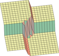
Figure 4: A generic view of the solution for $\rho=10^{-7}$. In the central (finite) region, the single shock prevails; this single shock matches with the two orthogonal shocks, which prevail instead in the outer region. In this figure: $\alpha=5,~{}\beta=4~{}(F=101),~{}\delta^{\pm}=1,~{}C=1,~{}\rho=10^{-7}$

References

- [1] M. Toda, Theory of Nonlinear Lattices (Springer-Verlag, Berlin Heidelberg, 1989).
- [2] M. Toda, Progress of Theoretical Physics Supplement 45, 174-200 (1970).
- [3] M. Toda and M. Wadati, J. Phys. Soc. Japan 34, 18-25 (1973).
- [4] R. Hirota, J. Phys. Soc. Japan 43, 2074-8 (1977); R. Hirota, J. Phys. Soc. Japan 45, 321-3 (1978).
- [5] D. Levi, L. Pilloni and P. M. Santini, J. Phys. A: Math. Gen. 14, 1567-75 (1981).
- [6] E. Date, M. Jimbo and T. Miwa, J. Phys. Soc. Jpn. 51, 4125-31 (1982).
- [7] R. Hirota, M. Ito and F. Kako, Progr. Theor. Phys. Suppl. 94, 42-58 (1988).
- [8] A. V. Mikhailov, Zh. Eksp. Teor. Fiz. 30, 443-448 (1979).
- [9] M. Bruschi, S. Manakov, O.Ragnisco and D.Levi, J. Math. Phys. 21, 2749 - 2753 (1980).
- [10] S. M. N. Ruijsenaars, Commun. Math. Phys. 133, 217-47 (1990).
- [11] Y.B. Suris, J. Phys. A: Math. Gen. 29, 451-465 (1996); 30 2235-2249 (1997).
- [12] R.I. Yamilov, in Proc eedings of 8th Workshop Nonlinear Evolution Equations and Dynamical Systems, (Singapore, World Scientific, 1993).
- [13] R. Hirota and K. Suzuki, Journal of the Physical Society of Japan 28, 1366-7 (1970).
- [14] R. Hirota and J. Satsuma, Prog. Theor. Phys. Suppl. 55, 64-100 (1976).
- [15] J.H.H. Perk, Phys.Lett. A 79 3-5 (1980); H. Au-Yang and J.H.H. Perk, Physica 144, 44-104 (1987).
- [16] G.W. Gibbons and K. Maeda, Nuclear Physics B 298 , 741-75 (1988).
- [17] H. Lu, C.N. Pope and K.W. Xu, Mod.Phys.Lett. A11, 1785-1796 (1996).
- [18] H. Lu and C.N. Pope Int.J.Mod.Phys. A12, 2061-2074 (1997).
- [19] A. Lukas, B.A. Ovrut and D. Waldram, Phys. Lett. B 393, 65-71 (1997).
- [20] M. Nieszporski, P. M. Santini and A. Doliwa, Phys. Lett. A 323, 241-250 (2004).
- [21] M. Laplace, Mémoires de Mathématique et de Physique de l’Académie des Sciences 341-403 (1773).
- [22] G. Darboux, L econs sur la Théorie Genérale des Surfaces (Paris:Gauthier-Villars, 1887).
- [23] X.-B. Hu, C.-X. Li, J.J.Nimmo and G.-F. Yu, A integrable symmetric (2+1)-dimensional Lotka-Volterra equation and a family of its solutions, preprint.
- [24] H. Flaschka, Prog. Theor. Phys. 51, 703-16 (1974).
- [25] S. V. Manakov, Soviet Phys. JETP 40, 269 (1975).
- [26] A. Doliwa, P. Grinevich, M. Nieszporski and P.M. Santini, Integrable lattices and their sublattices: from the discrete Moutard (discrete Cauchy-Riemann) equation to the self-adjoint 5-point scheme, (unpublished).
- [27] E. Date, M. Jimbo and T. Miwa, J. Phys. Soc. Japan 52, 766-771 (1983).
- [28] I.M. Krichever, Soviet Math. Dokl. 32, 623-627 (1985).
- [29] L. Bianchi, Lezioni di geometria differenziale, (Enrico Spoerri, Pisa, 1903), Vol II.
- [30] K. Maruno and G. Biondini, Resonance and web structure in discrete soliton systems: the two-dimensional Toda lattice and its fully discrete and ultra-discrete versions, nlin/0406059.