The Anti-FPU Problem

Abstract

We present a detailed analysis of the modulational instability of the zone-boundary mode for one and higher-dimensional Fermi-Pasta-Ulam (FPU) lattices. Following this instability, a process of relaxation to equipartition takes place, which we have called the Anti-FPU problem because the energy is initially fed into the highest frequency part of the spectrum, at variance with the original FPU problem (low frequency excitations of the lattice). This process leads to the formation of chaotic breathers in both one and two dimensions. Finally, the system relaxes to energy equipartition on time scales which increase as the energy density is decreased. We show that breathers formed when cooling the lattice at the edges, starting from a random initial state, bear strong qualitative similarities with chaotic breathers.

Keywords:Modulational instability, Localized modes, energy localization, energy equipartition, chaotic dynamics.

Several nonlinear physical systems exhibit modulational instability, which is a self-induced modulation of the steady state resulting from a balance between nonlinear and dispersive effects. This phenomenon has been studied in a large variety of physical contexts: fluid dynamics, nonlinear optics and plasma physics. The Fermi-Pasta-Ulam (FPU) lattice is an extremely well–suited model system to study this process. Both the triggering of the instability and its further evolution can be studied in detail, exciting initially high-frequency modes. The original FPU problem was casted instead in the context of long wavelengths. This is why we call the process we analyze in this paper, the Anti–FPU problem because of the analogy with the seminal FPU numerical simulation. At variance with the appearance of (m)KdV-solitons in the FPU original problem, in this process the pathway to equipartition leads to the creation of localized objects that are chaotic breathers. Similar localized structures emerge when cooling the lattice at the edges, starting from thermalized initial states.

I Introduction

In 1955, reporting about one of the first numerical simulations, Fermi, Pasta and Ulam (FPU) FPU remarked that it was $\ldots$ very hard to observe the rate of “thermalization” or mixing $\ldots$ in a nonlinear one-dimensional lattice in which the energy was initially fed into the lowest frequency mode. Even if the understanding of this problem advanced significantly afterwards ford ; lichtlieb , several issues are still far from being clarified. In most cases, the evolution towards energy equipartition among linear modes has been checked considering an initial condition where all the energy of the system is concentrated in a small packet of modes centered around some low frequency.

Beginning with the pioneering paper of Zabusky and Deem ZabuskyDeem , the opposite case in which the energy is put into a high frequency mode has been also analyzed. In this early paper, the zone–boundary mode was excited with an added spatial modulation for the one-dimensional $\alpha$-FPU model (quadratic nonlinearity in the equations of motion). Here, we will study the time-evolution of this mode without any spatial modulation for the $\beta$-FPU model (cubic nonlinearity in the equations of motion) and some higher–order nonlinearities. Moreover, we will extend the study to higher dimensional lattices. Since the energy is fed into the opposite side of the linear spectrum, we call this problem the Anti-FPU problem.

In a paper by Bundinsky and Bountis bountis , the zone–boundary mode solution of the one-dimensional FPU lattice was found to be unstable above an energy threshold $E_{c}$ which scales like $1/N$, where $N$ is the number of oscillators. This result was later and independently confirmed by Flach flach and Poggi et al. PR , who also obtained the correct factor in the large $N$-limit. These results were obtained by a direct linear stability analysis around the periodic orbit corresponding to the zone-boundary mode. Similar methods have been recently applied to other modes and other FPU-like potentials by Chechin et al chechin ; chechin2004 and Rink Rink2003 .

A formula for $E_{c}$, valid for all $N$, has been obtained in Refs. sandusky ; burlakov ; DRT ; Paladin in the rotating wave approximation, and will be also discussed in this paper. Associated with this instability is the calculation of the growth rates of mode amplitudes. The appropriate approach for Klein-Gordon lattices was first introduced by Kivshar and Peyrard KivsharPeyrard , following an analogy with the Benjamin-Feir instability in fluid mechanics benjaminFeir .

Previously, a completly different approach to describe this instability was introduced by Zakharov and Shabat zakharov , studying the associated Nonlinear Schrödinger equation in the continuum limit. A value for the energy threshold was obtained in Ref.lukomskii in the continuum limit. The full derivation starting from the FPU equation of motions was then independently obtained by Berman and Kolovskii berman in the so-called “narrow-packet” approximation.

Only very recently the study of what happens after modulational instability develops has been performed for Klein-Gordon daumont and FPU-latticesmaledetirusi ; sandusky . From these analyses it turned out that these high-frequency initial conditions lead to a completely new dynamical behavior in the transient time preceeding the final energy equipartition. In particular, the main discovery has been the presence on the lattice of sharp localized modes maledetirusi ; daumont . These latter papers were the first to make the connection between energy relaxation and intrinsic localized modes ST , or breathers diffflach1 ; diffflach2 ; diffflach3 ; reviewbreather . Later on, a careful numerical and theoretical study of the dynamics of a $\beta$-FPU model was performed cretegny . It has been shown that moving breathers play a relevant role in the transient dynamics and that, contrary to exact breathers, which are periodic solutions, these have a chaotic evolution. This is why they have been called chaotic breathers. Following these studies, Lepri and Kosevich kosevichlepri and Lichtenberg and coworkers ulman ; mirnov have further characterized the scaling laws of relaxation times using also continuum limit equations.

On the other hand, studies of the asymptotic state of the FPU lattice dynamics when energy is extracted from the boundaries have revealed the persistence of localized modes Aubry1 ; Aubry2 ; noi ; reigada1 ; noichaos . Already some of these authors noi ; noichaos have discussed the similarities of these modes with chaotic breathers. In this paper, we will further study this connection.

Most of the previous studies are for one-dimensional lattices. Here, we will derive modulational instability thresholds also for higher dimensional lattices and we will report on a study of chaotic breathers formation in two-dimensional FPU lattices.

We have organized the paper in the following way. In Section II, the modulational instability of zone-boundary modes on the lattice is discussed, beginning with the one-dimensional case, followed by the two-dimensional and higher dimensional cases and finishing with the continuum Nonlinear Schrödinger approach. Section III deals with the mechanisms of creation of chaotic breathers in one and two dimensions. Finally, in Section IV, we discuss the relation with numerical experiments performed when the lattice is cooled at the edges. Some final remarks and conclusions are reported in Section V.

II Modulational Instability

II.1 The one-dimensional case

We will discuss in this section modulational instability for the one-dimensional FPU lattice, where the linear coupling is corrected by a $(2p+1)$-th order nonlinearity, with $p$ a positive integer. Denoting by $u_{n}(t)$ the relative displacement of the $n$-th particle from its equilibrium position, the equations of motion are

$$\ddot{u}_{n}=u_{n+1}+u_{n-1}-2u_{n}+(u_{n+1}-u_{n})^{2p+1}-(u_{n}-u_{n-1})^{2p+1}.$$ (1)

We adopt a lattice of $N$ particles and we choose periodic boundary conditions. For the sake of simplicity, we first report on the analysis for $p=1$ (i.e. the $\beta$-FPU model) and then we generalize the results to any $p$-value.

Due to periodic boundary conditions, the normal modes associated to the linear part of Eq. (1) are plane waves of the form

$$u_{n}(t)={a\over 2}\left(e^{i\theta_{n}(t)}+e^{-i\theta_{n}(t)}\right)$$ (2)

where $\theta_{n}(t)=qn-\omega t$ and $q=2\pi k/N$ ($k=-N/2,\dots,N/2$). The dispersion relation of nonlinear phonons in the rotating wave approximation sandusky is $\omega^{2}(q)=4(1+\alpha)\sin^{2}(q/2)$, where $\alpha=3a^{2}\sin^{2}(q/2)$ takes into account the nonlinearity. Modulational instability of such a plane wave is investigated by studying the linearized equation associated with the envelope of the carrier wave (2). Therefore, one introduces infinitesimal perturbations in the amplitude and phase and looks for solutions of the form

$$u_{n}(t) = {a\over 2}[1+b_{n}(t)]\ e^{i\left[\theta_{n}(t)+\psi_{n}(t)\right]}+{a\over 2}[1+b_{n}(t)]\ e^{-i\left[\theta_{n}(t)+\psi_{n}(t)\right]}$$ (3)

$$= a[1+b_{n}(t)]\ \cos[qn-\omega t+\psi_{n}(t)],$$

where $b_{n}$ and $\psi_{n}$ are reals and assumed to be small in comparison with the parameters of the carrier wave. Substituting Eq. (3) into the equations of motion and keeping the second derivative, we obtain for the real and imaginary part of the secular term $e^{i(qn-\omega t)}$ the following equations

$$-\omega^{2}b_{n}+2\omega\dot{\psi}_{n}+\ddot{b}_{n} = (1+2\alpha)\left[\cos q\,(b_{n+1}+b_{n-1})-2b_{n}\right]$$ (4)

$$- \alpha\left(b_{n+1}+b_{n-1}-2b_{n}\cos q\right)-(1+2\alpha)\sin q\,(\psi_{n+1}-\psi_{n-1})$$

$$-\omega^{2}\psi_{n}-2\omega\dot{b}_{n}+\ddot{\psi}_{n} = (1+2\alpha)\left[\cos q\,(\psi_{n+1}+\psi_{n-1})-2\psi_{n}\right]$$ (5)

$$+ (1+2\alpha)\sin q\,(b_{n+1}-b_{n-1})+\alpha\left(\psi_{n+1}+\psi_{n-1}-2\psi_{n}\cos q\right).$$

Further assuming $b_{n}=b_{0}\ e^{i(Qn-\Omega t)}+{\rm c.c.}$ and $\psi_{n}=\psi_{0}\ e^{i(Qn-\Omega t)}+{\rm c.c.}$ we obtain the two following equations for the secular term $e^{i(Qn-\Omega t)}$

$$b_{0}\Bigl{[}\Omega^{2}+\omega^{2}+2(1+2\alpha)(\cos q\cos Q-1)-2\alpha(\cos Q-\cos q)\Bigr{]}-2i\psi_{0}\left[\omega\Omega+(1+2\alpha)\sin q\sin Q\right]=0$$ (6)

$$\psi_{0}\Bigl{[}\Omega^{2}+\omega^{2}+2(1+2\alpha)(\cos q\cos Q-1)+2\alpha(\cos Q-\cos q)\Bigr{]}+2ib_{0}\left[\omega\Omega+(1+2\alpha)\sin q\sin Q\right]=0.$$ (7)

In the case of Klein-Gordon type equations KivsharPeyrard ; daumont , one neglects the second order derivatives in Eqs. (4)-(5). This can be justified by the existence of a gap in the dispersion relation for $q=0$, which allows to neglect $\Omega^{2}$ with respect to $\omega^{2}$. In the FPU case, this approximation is worse, especially for long wavelengths, because there is no gap.

Non trivial solutions of Eqs. (6)-(7) can be found only if the Cramer’s determinant vanishes, i.e. if the following equation is fulfilled:

$$\Biggl{[}(\Omega+\omega)^{2}-4(1+2\alpha)\sin^{2}\left({q+Q\over 2}\right)\Biggr{]} \Biggl{[}(\Omega-\omega)^{2}-4(1+2\alpha)\sin^{2}\left({q-Q\over 2}\right)\Biggr{]}$$ (8)

$$= 4\alpha^{2}\left(\cos{Q}-\cos q\right)^{2}.$$

This equation admits four different solutions when the wavevectors $q$ of the unperturbed wave and $Q$ of the perturbation are fixed. If one of the solutions is complex, an instability of one of the modes $(q\pm Q)$ is present, with a growth rate given by the imaginary part of the solution. Using this method, one can derive the instability threshold amplitude for any wavenumber. A trivial example is the $q=0$ case, for which we obtain $\Omega=\pm\sin\left({Q/2}\right)$, which proves that the zero mode solution is stable. This mode is present due to the invariance of the equations of motion (1) with respect to the translation $u_{n}\to u_{n}+const$ and, as expected, is completely decoupled from the others.

A first interesting case is $q=\pi$. One can easily see that Eq. (8) admits two real and two complex conjugate imaginary solutions if and only if

$$\cos^{2}{Q\over 2}>{1+\alpha\over 1+3\alpha}.$$ (9)

This formula was first obtained by Sandusky and Page (Eq. (22) in Ref. sandusky ) using the rotating wave approximation. The first mode to become unstable when increasing the amplitude $a$ corresponds to the wavenumber $Q={2\pi/N}$. Therefore, the critical amplitude $a_{c}$ above which the $q=\pi$-mode looses stability is

$$a_{c}=\left({\sin^{2}\left({\pi/N}\right)\over 3\left[3\cos^{2}\left({\pi/N}\right)-1\right]}\right)^{1/2}.$$ (10)

This formula is valid for all even values of $N$ and its large $N$-limit is

$$a_{c}={\pi\over\sqrt{6}N}+O\left({1\over{N^{3}}}\right).$$ (11)

In Fig. 1, we show its extremely good agreement with the critical amplitude determined from numerical simulations. It is interesting to emphasize that the analytical formula (10) diverges for $N=2$, predicting that the $\pi$-mode is stable for all amplitudes in this smallest lattice. This is in agreement with the Mathieu equation analysis (see Ref. PR p. 265).

Figure 1: Modulational instability threshold amplitude for the $\pi$-mode versus the number of particles in the one-dimensional FPU lattice. The solid line corresponds to the analytical formula (10), the dashed line to its large $N$-estimate (11) and the diamonds are obtained from numerical simulations.

It is also interesting to express this result in terms of the total energy to compare with what has been obtained using other methods zakharov ; bountis ; berman ; flach ; PR . Since for the $\pi$-mode the energy is given by $E=N(2a^{2}+4a^{4})$, we obtain the critical energy

$$E_{c}={2N\over 9}\sin^{2}\left({\pi\over N}\right){7\cos^{2}\left({\pi/N}\right)-1\over\left[3\cos^{2}\left({\pi/N}\right)-1\right]^{2}}.$$ (12)

For large $N$, we get

$$E_{c}={\pi^{2}\over 3N}+O\left({1\over{N^{3}}}\right).$$ (13)

This asymptotic behavior is the same as the one obtained using the narrow packet approximation in the context of the Nonlinear Schrödinger equation by Berman and Kolovskii (Eq. (4.1) in Ref. berman ). The correct scaling behavior with $N$ of the critical energy has been also obtained by Bundinsky and Bountis (Eq. (2.22) in Ref. bountis ) by a direct linear stability analysis of the $\pi$-mode. The correct formula, using this latter method, has been independently obtained by Flach (Eq. (3.20)) in Ref. flach ) and Poggi and Ruffo (p. 267 of Ref. PR ). Recently, the $N^{-1}$-scaling of formula (13) has been confirmed using a different numerical method and, interestingly, it holds also for the $2\pi/3$ and $\pi/2$ modes Cafarella .

This critical energy is also very close to the Chirikov “stochasticity threshold” energy obtained by the resonance overlap criterion for the zone boundary modeizraeilchirikov . The stochasticity threshold phenomenon has been thoroughly studied for long wavelength initial conditions, and it has been clarified that it corresponds to a change in the scaling law of the largest Lyapunov exponentpettini . We will show in Section III that above the modulational instability critical energy for the $\pi$-mode one reaches asymptotically a chaotic state with a positive Lyapunov exponent, consistently with Chirikov’s result.

The above results can be generalized to nonlinearities of $2p+1$ order in the equations of motion (1). We limit the analysis to the $\pi$-mode, for which the instability condition (9) takes the form

$$\cos^{2}{Q\over 2}>{1+\alpha\over 1+(2p+1)\alpha},$$ (14)

where

$$\alpha={(2p+1)!\over p!(p+1)!}\,a^{2p}.$$ (15)

Hence the critical amplitude above which the $\pi$-mode is unstable is

$$a_{c}=\left[{p!(p+1)!\,\sin^{2}\left({\pi/N}\right)\over(2p+1)!\left[(2p+1)\cos^{2}\left({\pi/N}\right)-1\right]}\right]^{1/2},$$ (16)

leading to the large $N$ scaling

$$a_{c} \sim N^{-{1/p}}$$ (17)

$$E_{c} \sim N^{1-2/p}.$$ (18)

This scaling also corresponds to the one found in Ref. Kladko when discussing tangent bifurcations of band edge plane waves in relation with energy thresholds for discrete breathers. Their “detuning exponent” $z$ has a direct connection with the nonlinearity exponent $p=z/2$. We will see in Section II.2 that this analogy extends also to higher dimensions.

For fixed $N$, $a_{c}$ is an increasing function of the power of the coupling potential with the asymptotic limit $\lim_{p\to\infty}a_{c}=0.5$. Therefore, in the hard potential limit the critical energy for the $\pi$-mode increases proportionally to $N$. The fact that we find a higher energy region where the system is chaotic is not in contradiction with the integrability of the one-dimensional system of hard rodsrefhardrod , because in the present case we have also a harmonic contribution at small distances.

For the FPU-$\alpha$ model (quadratic nonlinearity in the equations of motion), the $\pi$-mode is also an exact solution which becomes unstable at some critical amplitude which, contrary to the case of the FPU-$\beta$ model, is $N$-independentsandusky ; chechin ; which means that the critical energy is proportional to $N$ and then that $\pi$-mode can be stable in some low energy density limit also in the thermodynamic limit.

It has also been realized PR ; marie ; julien ; chechin ; Shinohara ; Rink2003 that group of modes form sets which are invariant under the dynamics. The stability analysis julien ; chechin2004 of pair of modes has shown a complex dependence on their relative amplitudes. The existence of such invariant manifolds has also allowed to construct Birkhoff-Gustavson normal forms for the FPU model, paving the way to KAM theory Rink2000 .

II.2 Higher dimensions

In this section, we will first discuss modulational instability of the two-dimensional FPU model. The method presented in section II.1 can be easily extended and the global physical scenario is preserved. However, the scaling with $N$ of the critical amplitude changes in such a way to make critical energy constant, in agreement with the analysis of Ref. Kladko .

The masses lie on a two-dimensional square lattice with unitary spacing in the $(x,y)$ plane. We consider a small relative displacement $u_{n,m}$ ($n,m\in[1,N]$) in the vertical $z$-direction. Already with a harmonic potential, if the spring length at equilibrium is not unitary, the series expansion in $u_{n,m}$ of the potential contains all even powers. We retain only the first two terms of this series expansion. After an appropriate rescaling of time and displacements to eliminate mass and spring constant values, one gets the following adimensionallized equations of motions

$$\ddot{u}_{n,m} = u_{n+1,m}+u_{n-1,m}+u_{n,m+1}+u_{n,m-1}-4u_{n,m}$$ (19)

$$+\left(u_{n+1,m}-u_{n,m}\right)^{3}+\left(u_{n-1,m}-u_{n,m}\right)^{3}+\left(u_{n,m+1}-u_{n,m}\right)^{3}+\left(u_{n,m-1}-u_{n,m}\right)^{3}.$$

Considering periodic boundary conditions, plane waves solutions have the form

$$u_{n,m}=a\cos\left(q_{x}n+q_{y}m-\omega t\right).$$ (20)

In the rotating wave approximationsandusky , one immediately obtains the dispersion relation

$$\omega^{2}=4\sin^{2}{q_{x}\over 2}+4\sin^{2}{q_{y}\over 2}+12a^{2}\left[\sin^{4}{q_{x}\over 2}+\sin^{4}{q_{y}\over 2}\right],$$ (21)

which becomes exact for the zone-boundary mode $(q_{x},q_{y})=(\pi,\pi)$,

$$\omega_{\pi,\pi}^{2}=8(1+3a^{2}).$$ (22)

In order to study the stability of the zone-boundary mode, we adopt a slightly different approach. Namely, we consider the perturbed relative displacement field of the form

$$u_{n,m}=\left({a\over 2}+b_{n,m}\right)e^{i(\pi n+\pi m-\omega_{\pi,\pi}t)}+c.c.,$$ (23)

where $b_{n,m}$ is complex. This approach turns out to be equivalent to the one of Section II.1 in the linear limit.

Substituting this perturbed displacement field in Eqs. (19), we obtain

$$[1+2\alpha]\left[b_{n+1,m}+b_{n-1,m}+b_{n,m+1}+b_{n,m-1}+4b_{n,m}\right]$$

$$-\alpha\left[b^{*}_{n+1,m}+b^{*}_{n-1,m}+b^{*}_{n,m+1}+b^{*}_{n,m-1}+4b^{*}_{n,m}\right] =-\ddot{b}_{n,m}+2i\omega_{\pi,\pi}\dot{b}_{n,m}+\omega_{\pi,\pi}^{2}b_{n,m},$$ (24)

where $\alpha=3a^{2}$. Looking for solutions of the form

$$b_{n,m}=Ae^{i(Q_{x}n+Q_{y}m-\Omega t)}+Be^{-i(Q_{x}n+Q_{y}m-\Omega t)},$$ (25)

we arrive at the following set of linear algebraic equations for the complex constants $A$ and $B$

$$\left[(\Omega+\omega_{\pi,\pi})^{2}-8(1+2\alpha)\Delta\right]A+8\alpha\Delta B = 0$$ (26)

$$8\alpha\Delta A+\left[(\Omega-\omega_{\pi,\pi})^{2}-8(1+2\alpha)\Delta\right]B = 0,$$ (27)

where $2\Delta=\cos^{2}(Q_{x}/2)+\cos^{2}(Q_{y}/2)$. As for the one-dimensional case, we require that the determinant of this linear system in $A$ and $B$ vanishes, which leads to the following condition

$$\left[(\Omega+\omega_{\pi,\pi})^{2}-8\Delta(1+2\alpha)\right]\left[(\Omega-\omega_{\pi,\pi})^{2}-8\Delta(1+2\alpha)\right]=64\alpha^{2}\Delta^{2}.$$ (28)

This equation admits two real and two complex conjugated imaginary solutions in $\Omega$ if

$$\Delta>{1+\alpha\over 1+3\alpha},$$ (29)

which is the analogous for two dimensions of condition (9). One can achieve the minimal nonzero value of the r.h.s. of the above expression choosing $Q_{x}=0$, $Q_{y}=2\pi/{N}$, which leads to the following result for the critical amplitude

$$a_{c}=\left({\sin^{2}(\pi/{N})\over 3[3\cos^{2}(\pi/{N})+1]}\right)^{1/2}.$$ (30)

Its large $N$ limit is

$$a_{c}={\pi\over\sqrt{12}N}+O\left({1\over{N^{3}}}\right).$$ (31)

This prediction is compared with numerical data in Fig. 2. The agreement is good for all values of $N$.

Since the relation between energy and amplitude is now $E=2N^{2}(2a^{2}+4a^{4})$, we obtain the critical energy in the large $N$-limit as

$$E_{c}={\pi^{2}\over 3}+O\left({1\over{N^{2}}}\right).$$ (32)

This shows that the critical energy is now constant in the thermodynamic limit, which agrees with the remark of Ref. Kladko about the existence of a minimal energy for breathers formation reviewbreather .

The results of this Section can be easily extended to any dimension $d$. Repeating the same argument, we arrive at the following estimates for the critical amplitude and energy in the large $N$ limit

$$a_{c} = {\pi\over\sqrt{6d}}{1\over N}+O\left({1\over{N^{3}}}\right)$$ (33)

$$E_{c} = {\pi^{2}\over 3}N^{d-2}+O\left({N^{d-4}}\right).$$ (34)

This means that the critical energy density $\varepsilon_{c}=E_{c}/N$ for destabilizing the zone boundary mode vanishes as $1/N^{2}$, independently of dimension.

Figure 2: Modulation instability threshold for the $(\pi,\pi)$ mode versus number of oscillators in two dimensional array. The solid line is given by the corresponds to the estimate obtained from the Nonlinear Schrödinger equation in large $N$ limit (see formula (43)) and the diamonds are results of numerical simulations.

II.3 Large $N$ limit using the Nonlinear Schrödinger equation

The large $N$ limit expressions (33) and (34) can be derived also by continuum limit considerations. We will derive the general expression for any dimension $d$. The displacement field can be factorized into a complex envelope part $\psi$ multiplied by the zone boundary mode pattern in $d$ dimensions.

$$u_{n_{1},\dots,n_{d}}={\psi(n_{1},\dots,n_{d},t)\over 2}e^{i\left(\pi\sum_{i=1}^{d}n_{i}-\omega_{\pi,\dots,\pi}t\right)}+c.c.\ ,$$ (35)

where

$$\omega_{\pi,\dots,\pi}=\sqrt{d\left[4(1+3|\psi|^{2})\right]}.$$ (36)

Substituting Eq. (35) into the FPU lattice equations in $d$ dimensions, a standard procedure RemoissenetSemiDis ; book leads to the following $d$ dimensional Nonlinear Schrödinger (NLS) equation:

$$i{\partial\psi\over\partial t}+{P\over 2}\,\Delta_{d}\psi-Q\psi{\left|\psi\right|}^{2}=0,$$ (37)

where $\Delta_{d}$ is the $d$ dimensional Laplacian. The parameters $P$ and $Q$ are derived from the nonlinear dispersion relation

$$\omega^{2}=\sum_{i=1}^{d}\left[4\sin^{2}{q_{i}\over 2}+12|\psi|^{2}\sin^{4}{q_{i}\over 2}\right],$$ (38)

as

$$P = {\partial^{2}\omega\over\partial q_{i}^{2}}\left({q_{1}=\pi,\dots,q_{d}=\pi,|\psi|=0}\right)={1\over 2\sqrt{d}}$$ (39)

$$Q = -{\partial\omega\over\partial|\psi|^{2}}\left({q_{1}=\pi,\dots,q_{d}=\pi,|\psi|=0}\right)=-3\sqrt{d}.$$ (40)

Assuming that, at the first stage, modulational instability develops along a single direction $x$ and that the field remains constant along all other directions, one gets the one-dimensional NLS equation

$$i{\partial\psi\over\partial t}+{P\over 2}{\partial^{2}\psi\over\partial x^{2}}-Q\psi{\left|\psi\right|}^{2}=0.$$ (41)

Following the results of the inverse scattering approach zakharov , any initial distribution of amplitude $|\psi|$ and length $\lambda$ along $x$, and constant along all other directions, produces a final localized distribution if lukomskii

$$(|\psi|\lambda)^{2}>\pi^{2}\left|{P\over Q}\right|.$$ (42)

This means that if the initial state is taken with constant amplitude $|\psi|=a$ on the $d$-dimensional lattice with $N^{d}$ oscillators, the modulational instability threshold is

$$(a_{c}{N})^{2}={\pi^{2}\over 6d}$$ (43)

which coincides with the leading order in Eq. (33).

III Chaotic Breathers

In this Section, we will discuss what happens when the modulational energy threshold is overcome. The first thorough study of this problem can be found in Ref. maledetirusi , many years after the early pioneering work of Zabusky and Deem ZabuskyDeem . Already in Ref. maledetirusi , it has been remarked that an energy localization process takes place, which leads to the formation of breathers reviewbreather . This process has been further characterized in terms of time-scales to reach energy equipartition and of quantitative localization properties in Ref. cretegny . The localized structure which emerges after modulational instability has been here called “chaotic breather” (CB). The connection between CB formation and continuum equations has been discussed in Refs. kosevichlepri ; mirnov , while the relation with the process of relaxation to energy equipartition has been further studied in Ref. ulman . We will briefly recall some features of the localization process in one dimension and present new results for two dimensions.

For long time simulations, we use appropriate symplectic integration schemes in order to preserve as far as possible the Hamiltonian structure. For the one dimensional FPU, we adopt a 6th-order Yoshida’s algorithm yoshida with a time step $dt=0.01$; this choice allows us to obtain an energy conservation with a relative accuracy $\Delta E/E$ ranging from $10^{-10}$ to $10^{-12}$. For two dimensions, we use instead the 5–th order symplectic Runge–Kutta–Nyström algorithm of Ref. Calvo , which gives a similar quality of energy conservation.

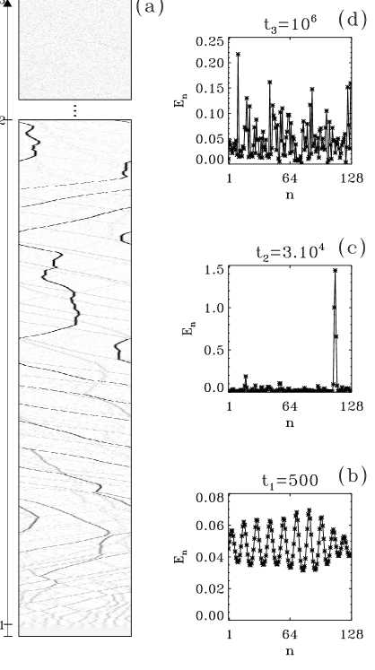
Figure 3: Time evolution of the local energy (44). In panel (a), the horizontal axis indicates lattice sites and the vertical axis is time. The grey scale goes from $E_{n}=0$ (white) to the maximum $E_{n}$-value (black). The lower rectangle corresponds to $0<t<3\ 10^{4}$ and the upper one to $0.994\ 10^{6}<t<10^{6}$. Figs. (b), (c) and (d) show the instantaneous local energy $E_{n}$ along the $N=128$ chain at three different times. Remark the difference in vertical amplitude in panel (c), when the chaotic breather is present. The initial $\pi$-mode amplitude is $a=0.15>a_{c}\simeq 0.01$.

We report in Fig. 3(a) a generic evolution of the one dimensional $\pi$-mode above the modulation instability critical amplitude ($a>a_{c}$). The grey scale refers to the energy residing on site $n$,

$$E_{n}={1\over 2}\dot{u}_{n}^{2}+{1\over 2}V(u_{n+1}-u_{n})+{1\over 2}V(u_{n}-u_{n-1}),$$ (44)

where the FPU-potential is $V(x)={1\over 2}x^{2}+{1\over 4}x^{4}$. Figs. 3(b), 3(c) and 3(d) are three successive snapshots of the local energy $E_{n}$ along the chain. At short time, a slight modulation of the energy in the system appears (see Fig. 3(b)) and the $\pi$-mode is destabilized sandusky . Later on, as shown in Fig. 3(a), only a few localized energy packets emerge: they are breathers reviewbreather . Inelastic collisions of breathers have a systematic tendency to favour the growth of the big breathers at the expense of small ones prllocali ; BangPeyrard . Hence, in the course of time, the breather number decreases and only one, of very large amplitude, survives (see Fig. 3(c)): this is the localized excitation we have called chaotic breather (CB). The CB moves along the lattice with an almost ballistic motion: sometimes it stops or reflects. During its motion the CB collects energy and its amplitude increases. It is important to note that the CB is never at rest and that it propagates with a given subsonic speed KosevichCorso . Finally, the CB decays and the system reaches energy equipartition, as illustrated in Fig. 3(d). The final CB decay is present in all the simulations we have performed, but one cannot exclude the existence of examples where the final breather does not disappear.

In order to obtain a quantitative characterization of energy localization, we introduce the “participation ratio”

$$C_{0}(t)=N{\displaystyle\sum_{i=1}^{N}E_{i}^{2}\over\left(\displaystyle\sum_{i=1}^{N}E_{i}\right)^{2}},$$ (45)

which is of order one if $E_{i}=E/N$ at each site of the chain and of order $N$ if the energy is localized on only one site. In Fig. 4(a), $C_{0}$ is reported as a function of time. Initially, $C_{0}$ grows, indicating that the energy, evenly distributed on the lattice at $t=0$, localizes over a few sites. This localized state survives for some time. At later times, $C_{0}$ starts to decrease and finally reaches an asymptotic value $\bar{C}_{0}$ which is associated with the disappearance of the CB (an estimate of $\bar{C}_{0}$ has been derived in Ref. cretegny taking into account energy fluctuations and is reported with a dashed line in Fig. 4(a)). At this stage, the energy distribution in Fourier space is flat, i.e. a state of energy equipartition is reached.

As explained in Ref. cretegny , the destruction of the breathers is related to its interaction with low frequency modes which are dominant in the chain after the initial stage. A full study of the scattering of plane waves by FPU-breathers would be necessary to quantify this explanation either as anticipated in Ref. cretegny or, even better, as recently performed by Flach and collaborators for the discrete NLS equation, Klein-Gordon or FPU chains flachandrei ; flachandreiFPU .

In Fig. 4(b), we show the finite time largest Lyapunov exponent $\lambda_{1}(t)$ for the same orbit as in Fig. 4(a). We observe a growth of $\lambda_{1}(t)$ when the CB emerges on the lattice and a decrease when it begins to dissolve. The peak in $\lambda_{1}(t)$ perfectly coincides with the one in $C_{0}$. Due to this increase of chaos associated with localization, we have called the breather chaotic (although chaos increase could be the result of a more complicated process of interaction with the background).

In Ref. cretegny , the time-scale for the relaxation to equipartition has been found to increase as $(E/N)^{-2}$ in the small energy limit. This has been confirmed by the followers of this study kosevichlepri ; ulman ; mirnov . Such power law scalings are found also for the FPU relaxation starting from long wavelengths delucca : the so-called FPU problem. We have termed the relaxation process which starts from short wavelengths the Anti-FPU problem, just because of the similarities in the scaling laws. The main feature of the latter problem is that relaxation to equipartition goes through a complex process of localized structures formation well described by breathers or, in the low-amplitude limit, by solitons of the NonLinear Schrodinger equation. On the contrary, for the original FPU problem, an initial long wavelength excitation breaks up into a train of mKdV-solitons. The final relaxation to equipartition is however due to an energy diffusion process which has similar features for both the FPU and the Anti-FPU problem ulman .

Figure 4: Panel (a) presents the evolution of $C_{0}(t)$ of formula (45) for the one-dimensional FPU lattice with $N=128$ oscillators, initialized on the $\pi$-mode with an amplitude $a=0.126>a_{c}\simeq 0.010$. The dashed line indicates the equilibrium value $\bar{C}_{0}=1.795$. Panel (b) presents the corresponding finite time largest Lyapunov exponent. Panel (c) shows $C_{0}(t)$ for the two-dimensional FPU lattice with $20*20$ oscillators, initialized on the $(\pi,\pi)$-mode with an amplitude $a=0.425>a_{c}\simeq 0.045$. Panel (d) presents the finite time largest Lyapunov exponent for two dimensions.

A similar evolution of the local energy

$$E_{n,m}={1\over 2}\dot{u}_{n,m}^{2} +{1\over 4}V(u_{n+1,m}-u_{n,m})+{1\over 4}V(u_{n,m+1}-u_{n,m})$$ (46)

$$+{1\over 4}V(u_{n-1,m}-u_{n,m})+{1\over 4}V(u_{n,m-1}-u_{n,m})$$

is observed for the two-dimensional case (see Fig. 5). In this figure, we just show the initial evolution which leads to breathers formation. As for the one-dimensional case, bigger breathers eat up smaller ones, and finally only one breather survives. However, note that, depending on the initial conditions, the simulations do not always lead to the coalescence into a single breather, because collisions are more rare in two dimensions than in one. After the formation of a few localized structures, one also observes the final relaxation to equipartition, which is not shown in Fig. 5. This latter is instead evident from the time evolution of $C_{0}(t)$, the localization parameter, shown in Fig. 4(c): its behavior is very similar to the one-dimensional case. Indeed, also the largest finite time Lyapunov exponent behaves similarly (see Fig. 4(d)).

Figure 5: Local energy (46) surface plots for the two-dimensional FPU lattice with $20*20$ oscillators, initialized on the $(\pi,\pi)$-mode with an amplitude $a=0.225>a_{c}\simeq 0.045$. Snapshots at four different times $t$ are shown. Breathers form after a coalescence process similarly to the one-dimensional case. The mobility of the breathers is evident and one also observes in the last panel the final decrease.

IV Spontaneous localization by edge cooling

Breathers play an important role in the non–equilibrium dynamics of the FPU model. The relaxation to equipartition of the zone–boundary mode, analyzed thus far in this paper, is one example. Another interesting case in which breathers emerge spontaneously is when the lattice is cooled at its boundaries Aubry1 ; Aubry2 ; noi ; reigada1 ; noichaos . This process may be thought of as modeling a non–equilibrium process where energy exchange in the bulk is much slower than at the surface. Although in this case the dynamics is dissipative, it turns out that there is a deep connection with the original Hamiltonian model.

Specifically, when modelling this process, we add a dissipative term $-\eta\dot{u}_{n}$ in the r.h.s. of Eq. (1) when $n=1$ and $n=N$. Similarly, in two dimensions, the same term is introduced at all edge sites. The parameter $\eta$ controls the strength of the coupling with the external reservoirs at zero temperature. Since we are interested in the exchange of energy between a finite system and the environment, we shall consider either free–ends or fixed–ends boundary conditions.

In a typical simulation, first an equilibrium micro-state is generated by letting the Hamiltonian system ($\eta=0$) evolve for a sufficiently long transient. Then, the dissipative dynamics ($\eta>0$) is started. The initial condition for the Hamiltonian transient is assigned by setting all relative displacements to zero and by drawing velocities at random from a Gaussian distribution. The velocities are then rescaled by a suitable factor to fix the desired value of the initial energy $E(0)$ (see Ref. noi for the details).

The one-dimensional numerical simulations reveal that the dissipation rate of the energy is dominated by two sequential effects, that characterize the pathway to localization. In the first stage of the energy release process, the relaxation law undergoes a crossover from the exponential $\exp[-t/\tau_{\scriptscriptstyle 0}]$ to the power law $(t/\tau_{\scriptscriptstyle 0})^{-1/2}$, where $\tau_{\scriptscriptstyle 0}=N/(2\eta)$ sets the shortest time scale of the system (see Fig. 6) noichaos . Asymptotically, energy reaches a plateau and, correspondingly, the localization parameter $C_{0}(t)$ also saturates (see the inset of Fig. 6).

The crossover at $\tau_{\scriptscriptstyle 0}$ is a signature of the hierarchical nature of the early stages of the process. In the harmonic approximation, if one adds a small dissipation, the frequency $\omega$ of each linear mode acquires an imaginary part $\gamma(\omega)$, which represents its damping rate. Initially, it is only the fastest mode which determines the energy relaxation rate. As time goes on, past $t\simeq\tau_{\scriptscriptstyle 0}$, it is the full spectrum of decay times of the linear modes that sets the rules of energy relaxation. Actually, it turns out that at this stage, for small nonlinearities, the system behaves approximately as its linear counterpart (see Fig. 6). In particular, a perturbative calculation to first order in $\gamma$ confirms that noichaos

$${E(t)\over E(0)} \equiv \int e^{\displaystyle-\gamma(\omega)t}\,g(\omega)\,d\omega\simeq\begin{cases}e^{\displaystyle-t/\tau_{\scriptscriptstyle 0}}&\text{for $t\ll\tau_{\scriptscriptstyle 0}$}\\ {\displaystyle 1\over\displaystyle\sqrt{2\pi t/\tau_{\scriptscriptstyle 0}}}&\text{for $t\gg\tau_{\scriptscriptstyle 0}$}\end{cases},$$ (47)

where the density of states $g(\omega)$ is derived from the dispersion relation $\omega(q)=2\sin(q/2)$, with $q=\pi k/N$ for free–ends boundary conditions, and $q=\pi(k+1)/(N+1)$ for fixed–ends boundary conditions ($k=0,\dots N-1$).

The time range after the crossover coincides with the onset of localization. Now the dynamics is significantly affected by the spontaneous appearance of breathers. As the latter exhibit a very weak interaction among themselves and with the boundaries, the energy release undergoes a slowing down, thus freezing the system in a quasi–stationary configuration far from thermal equilibrium.

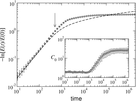
Figure 6: Log–log plot of $-\log[E(t)/E(0)]$ versus time for an FPU chain with free–ends boundary conditions. In this representation, an exponential is a straight line with slope one. Symbols are the results of numerical simulations averaged over 20 initial conditions. The dashed line is a plot of the theoretical result (47) noi for a harmonic chain. The arrow indicates the crossover time $\tau_{0}$. Parameters are $N=100$ and $\eta=0.1$.

Such residual state is characterized by the presence of one, highly energetic localized object (possibly accompanied by a few much smaller ones), which is mobile and alternates periods of rest and erratic motion, as shown in Fig. 7. This behaviour is reminiscent of the chaotic breathers which emerge in the Hamiltonian system from modulational instability of band–edge modes, discussed in Section III (see also Fig. 3).

Figure 7: Space–time contour plot of the site energies (44). Time flows up and the horizontal axis is the site index. Parameters are $N=100$, $\eta=0.1$ and $E(0)/N=1$.

But what do we know of the mechanisms leading to spontaneous localization in the presence of dissipation? As noticed above, there is evidence that it is the modulation instability of short lattice waves that triggers the formation of localized structures. This hypothesis is supported by the observation that the emergence of spatial patterns in the early stages of the relaxation is intimately related to how dissipation acts on vibrational modes of different wavelength. In particular, if the system is swiftly enough depleted of long–wavelength modes, the instability associated with the band–edge waves may effectively trigger the process of localization. A key test for the above hypothesis is offered by the nature of the boundary conditions. In the case of free–ends, the modes of small wavenumber indeed disappear very fast, in conjunction with the onset of spontaneous localization. On the contrary, in the presence of fixed boundaries the former turn out to be as long–lived as the modes with large wavenumbers. The corresponding numerical evidence is that hardly no localization is observed in this case. Rather, the energy decays following exactly the behavior of the harmonic chain (47) noi . This scenario can be observed directly, by computing the time–dependent spatial power spectrum $S(q,t)$ during the relaxation (see Fig. 8).

Figure 8: Surface plot of the time–dependent spatial spectrum of particle velocities for the one-dimensional FPU lattice. (a) Fixed–ends boundary conditions. (b) Free–ends boundary conditions. Parameters are $N=100$, $\eta=0.1$ and $E(0)/N=1$.

It is possible to get a quantitative confirmation of the above hypothesis by calculating the exact relaxation spectrum $\gamma(\omega)$ of the linearized system. In the harmonic approximation, the equations of motion may be written in matrix form as

$$\dot{U}=\mathbb{A}\,U,$$ (48)

where $U=(u_{1},\dots,u_{N},\dot{u}_{1},\dots,\dot{u}_{N})^{T}$ is a $2N$ column vector, and $\mathbb{A}$ is the matrix

$$\mathbb{A}=\left(\vbox{\hbox{\hbox to0.0pt{\hbox{\kern 0.0pt\hbox{\vbox{\vbox{}\hrule width=0.0pt,height=0.0pt,depth=0.0pt}\kern 0.0pt\hbox{}}}\hss}\hbox to0.0pt{\vbox{}\hss}\vbox{\kern 0.0pt}}}\right)\quad.$$ (49)

The tri–diagonal matrix of force constants $K_{nm}$ also contains the information on the type of boundary conditions, whereas the matrix $B_{nm}=\delta_{nm}(\delta_{m1}+\delta_{mN})$ describes the coupling with the environment. The spectrum of damping rates can be calculated by straight diagonalization of matrix $\mathbb{A}$. In Fig. 9 we plot $\gamma(\omega)$, where $\gamma$ is the opposite of the real part of an eigenvalue of $\mathbb{A}$ and $\omega$ its imaginary part. This representation of the relaxation spectrum is preferable with respect to the one in terms of wave-numbers, since the vibration frequencies are shifted as a consequence of the damping.

This calculation confirms that the free–ends and fixed–ends systems display considerably different behaviors. In the former case, the least damped modes are the short–wavelength ones ($\omega\approx 2$, the band–edge frequency), the smallest damping constant being $\gamma(2)\approx\pi^{2}\eta/2N^{3}$, while the most damped modes are the ones in the vicinity of $\omega\sim 1/N$. On the contrary, for fixed ends, the most damped modes are those around the band center ($\omega\sim\sqrt{2}$) while both short– and long–wavelength waves dissipate very weakly ($\gamma\sim 1/N^{3})$.

Figure 9: Damping rates $\gamma(\omega)$ for an harmonic chain with $N=100$ and $\eta=0.1$. Free–ends boundary conditions (stars) and fixed–ends boundary conditions (diamonds).

The above analysis helps understanding why spontaneous localization is strongly inhibited if the system is trapped between rigid walls, thus in parallel unveiling the role of modulational instability in the process.

We have also performed similar numerical simulations for the two-dimensional FPU model (19), with dissipation added at the edges and free–ends boundary conditions. Remarkably, the asymptotic scenario changes. The quasi–stationary state is now a static collection of tightly–packed localized objects, arranged in a sort of random lattice (see Fig. 10). Moreover, it turns out that spontaneous localization in two dimensions is a thermally–activated phenomenon, described by an Arrhenius law for the average breather density, where the parameter that controls the strength of thermal fluctuations is the initial energy density $E(0)/N$ noichaos . The origin of this behaviour is that, in the two-dimensional FPU system, discrete breathers may be excited only above a certain energy threshold Kladko , as discussed in Section II.2. Despite the different nature of the asymptotic state, the onset of localization follows the same path in one and two dimensions noichaos , well described the hierarchy of relaxation times underlying Eq. (47). In particular, a crossover is observed from the exponential $\exp[-2t/\tau_{\scriptscriptstyle 0}]$ to the power law $(t/\tau_{\scriptscriptstyle 0})^{-1}$.

Figure 10: 2D FPU lattice, site energies in the residual state state. Parameters are: $N=80$, $\eta=0.1$, $E(0)/N=1$.

V Conclusions

In this paper, we have presented a detailed analysis of the zone-boundary mode modulational instability for the FPU lattice in both one and higher dimensions. Formulas for the critical amplitude have been derived analytically and compare very well with numerics for all system sizes. We have extended to two dimensions the study of the process which leads to the formation of chaotic breathers. The physical picture is similar to the one-dimensional case. Besides that, we make the bridge between breathers created by modulational instability of plane waves and the ones formed when extracting energy from the boundaries: similarities and differences are highlighted.

All results on modulational instability of zone-boundary modes can be straightforwardly extended to other initial modes and, correspondingly, instability rates can be derived. This has already partially been done in Ref. Paladin and compares very well with the numerical results by Yoshimura yoshi2 . This author has recently reanalyzed the problem yoshi3 to determine the growth rates for generic nonlinearities in the high energy region, obtaining exact results based on Mathieu’s equation.

Going to many–modes initial excitations, it has been remarked that instability thresholds depend on relative amplitudes and not only on the total energy chechin2004 . Although this makes the study of the problem extremely involved, we believe that a detailed study of some selected group of modes, which play some special role in FPU dynamics, could be interesting. The method discussed in this paper could be adapted to treat this problem. Historically, the first study is in the paper by Bivins, Metropolis and Pasta himself bivins , where the authors tackle the problem by studying numerically the instabilities of coupled Mathieu’s equations.

The study we have presented in this paper of the two-dimensional FPU lattice is extremely preliminary and further analyses are needed. In particular, the full process of relaxation to energy equipartion and the associated time scales have not been studied at all. Preliminary results on the relaxation process in two dimensions from low frequency initial states seem to indicate a faster evolution to equipartition benettin . A similar analysis for high frequencies remains to be performed.

In one-dimensional studies, a connection between the average modulation instability rates and the Lyapunov exponents has been suggested DRT ; Paladin . Recently franzozi , high frequency exact solutions have been used in the context of a differential geometric approach pettinilyap to obtain accurate estimates of the largest Lyapunov exponent. Similar studies could be performed for the two-dimensional FPU lattice and the corresponding scaling laws with respect to energy density could be obtained.

The study we have reported in the last Section about lattices that are cooled at the boundaries points out the similarity of the localized objects obtained in the long time limit with chaotic breathers. However, this resemblance, although convincing, is only qualitative. Quantitative studies on the comparison of these breathers with the chaotic ones obtained from modulational instability should be performed.

Acknowledgement: First, we would like to thank D. K. Campbell, P. Rosenau and G. Zaslavsky for the opportunity they gave us to contribute to this Chaos issue celebrating the anniversary of the FPU experiment. Then, we express our gratitude to all our collaborators in this field: J. Barré, M. Clément, T. Cretegny, S. Lepri, R. Livi, P. Poggi, A. Torcini. We also thank N. J. Zabusky for useful exchanges of informations and Zhanyu Sun for an important comment. This work is part of the contract COFIN03 of the Italian MIUR Order and chaos in nonlinear extended systems. R.Kh. is supported by NATO reintegration grant No. FEL.RIG.980767. S.R. thanks ENS Lyon for hospitality and financial support.

References

- (1) E. Fermi, J. Pasta, S. Ulam, Los Alamos Science Laboratory Report No. LA-1940 (1955), unpublished; reprinted in Collected Papers of Enrico Fermi, edited by E. Segré (University of Chicago Press, Chicago, 1965), Vol. 2, p 978. also in Nonlinear Wave Motion, Newell A. C. Ed., Lecture in Applied Mathematics 15 (AMS, Providence, Rhode Island, 1974) and in The Many-Body Problem, Mattis C. C. Ed. (World Scientific, Singapore, 1993).
- (2) A. J. Lichtenberg, M. A. Lieberman, Regular and chaotic dynamics (Springer, Berlin, 1992). Chapt. 6.5.
- (3) J. Ford, Phys. Rep. 213, 271 (1992).
- (4) N. J. Zabusky, G. S. Deem, J. Comp. Phys. 2, 126 (1967).
- (5) N. Budinsky, T. Bountis, Physica D 8, 445 (1983).
- (6) S. Flach, Physica D 91, 223 (1996).
- (7) P. Poggi, S. Ruffo, Physica D 103, 251 (1997).
- (8) G. M. Chechin, N. V. Novikova, A. A. Abramenko, Physica D 166, 208 (2002).
- (9) G. M. Chechin, D. S. Ryabov, K. G. Zhukov, nlin.ps/0403040 (2004).
- (10) B. Rink, Physica D 175, 31 (2003)
- (11) T. Dauxois, S. Ruffo, A. Torcini, Phys. Rev. E 56, R6229 (1997).
- (12) V. M. Burlakov, S. A. Darmanyan, V. N. Pyrkov, Sov. Phys. JETP 81, 496 (1995).
- (13) K. W. Sandusky, J. B. Page, Phys. Rev. B 50, 866 (1994).
- (14) T. Dauxois, S. Ruffo, A. Torcini, Journal de Physique IV 8, 147 (1998).
- (15) Yu. S. Kivshar, M. Peyrard, Phys. Rev. A 46, 3198 (1992).
- (16) T. B Benjamin, J. E. Feir, J. Fluid Mech. 27, 417 (1967).
- (17) V.E. Zakharov, A.B. Shabat, Zhurnal Eksperimentalnoi I Teoreticheskoi Fiziki 64, 1627 (1973).
- (18) V.P. Lukomskii, Ukr. Fiz. Zh. 23, 134 (1978).
- (19) G. P. Berman, A. R. Kolovskii, Zh. Eksp. Teor. Fiz. 87 , 1938 (1984) [Sov. Phys. JETP 60, 1116 (1984)].
- (20) I. Daumont, T. Dauxois, M. Peyrard, Nonlinearity 10, 617 (1997).
- (21) V. M. Burlakov, S. A. Kiselev, V. I. Rupasov, Phys. Lett. A 147, 130 (1990); V. M. Burlakov and S. Kiselev, Sov. Phys. JETP 72, 854 (1991).
- (22) A. J. Sievers, S. Takeno, Phys. Rev. Lett. 61, 970 (1988).
- (23) S. Aubry, Physica D 103, 201 (1997).
- (24) S. Flach, C. R. Willis, Physics Reports 295, 181 (1998).
- (25) D. K. Campbell, S. Flack, Yu. S. Kivshar, Physics Today, 43, January (2004).
- (26) T. Dauxois, A. Litvak-Hinenzon, R. S. MacKay, A. Spanoudaki (Eds), Energy Localisation and Transfer, Advanced Series in Nonlinear Dynamics, World Scientific (2004).
- (27) T. Cretegny, T. Dauxois, S. Ruffo, A. Torcini, Physica D 121, 109-126 (1998).
- (28) Y. A. Kosevich, S. Lepri, Phys. Rev. B 61, 299 (2000).
- (29) K. Ullmann, A. J. Lichtenberg, G. Corso, Phys. Rev. E 61, 2471 (2000).
- (30) V. V. Mirnov, A. J. Lichtenberg, H. Guclu, Physica D 157, 251 (2001).
- (31) G. P. Tsironis, S. Aubry Phys. Rev. Lett. 77 (26) 5225 (1996).
- (32) A. Bikaki, N. K. Voulgarakis, S. Aubry, G. P. Tsironis, Phys. Rev. E 59 (1) 1234 (1999).
- (33) F. Piazza, S. Lepri, R. Livi, J. Phys. A, 34, 9803 (2001).
- (34) F. Piazza, S. Lepri, R. Livi, Chaos - Focus Issue ”Nonlinear localised modes, Fundamental Concepts and Applications”, 13(2), 637 (2003).
- (35) R. Reigada, A. Sarmiento, K. Lindenberg, Phys. Rev. E 64 066608 (2001).
- (36) A. Cafarella, M. Leo, R. A. Leo, Phys. Rev. E 69, 046604 (2004).
- (37) F. M. Izraïlev, B. V. Chirikov, Dokl. Akad. Nauk. SSSR 166, 57 (1966) [Sov. Phys. Doklayd 11, 30 (1966)].
- (38) M. Pettini, M. Landolfi, Phys. Rev. A 41, 768 (1990).
- (39) S. Flach, K. Kladko, R. S. MacKay, Phys. Rev. Lett. 78, 1207 (1997).
- (40) D. W. Jepsen, J. Math. Phys. 6, 405 (1965).
- (41) J. Barré, rapport de stage de Maîtrise, ENS Lyon, “Instabilités des solutions périodiques et formation de breathers chaotiques dans le modèle FPU” (1998).
- (42) M. Clément, rapport de stage de License, ENS Lyon, “Différentes études du modèle Fermi-Pasta-Ulam” (1996).
- (43) S. Shinohara, J. Phys. Soc. Japan 71, 1802 (2002); Prog. Theor. Phys. Suppl. 150 423 (2003).
- (44) B. Rink, F. Verhulst, Physica A 285, 467 (2000); B. Rink, Comm. Math. Phys. 218, 665 (2001).
- (45) M. Peyrard, T. Dauxois, Physique des Solitons, CNRS Editions-EDP Sciences (2004)
- (46) M. Remoissenet, Phys. Rev. B 33, 2386 (1986).
- (47) H. Yoshida, Phys. Lett. A 150, 262 (1990).
- (48) J. M. Sanz–Serna, M. P. Calvo, Numerical Hamiltonian Problems, (London: Chapman & Hall) (1994).
- (49) T. Dauxois, M. Peyrard, Phys. Rev. Lett. 70, 3935 (1993).
- (50) O. Bang, M. Peyrard, Phys. Rev. E53, 4143 (1996).
- (51) Y. A. Kosevich, G. Corso, Physica D 170, 1 (2002).
- (52) J. DeLuca, A. J. Lichtenberg, S. Ruffo, Phys. Rev. E 60, 3781 (1999).
- (53) S. Flach, A. E. Mirochnishenko, M. V. Fistul, Phys. Rev. Lett. 90, 084101 (2003).
- (54) S. Flach, A. E. Mirochnishenko, M. V. Fistul, Chaos 13, 596 (2003).
- (55) K. Yoshimura, Physica D 104, 148 (1997).
- (56) K. Yoshimura, Phys. Rev. E 70, 016611 (2004).
- (57) R. L. Bivins, N. Metropolis, John R. Pasta, J. Comp. Phys. 12, 62 (1972).
- (58) G. Benettin, private communication (2004).
- (59) R. Franzosi, P. Poggi, M. Cerruti-Sola, nlin.cd/0408056 (2004).
- (60) M. Pettini, Phys. Rev. E 47, 828 (1993); L. Casetti, C. Clementi, M. Pettini, Phys. Rev. E 54, 5969 (1996).