Clustering transition in a system of particles self-consistently driven by a shear flow

Abstract

We introduce a simple model of active transport for an ensemble of particles driven by an external shear flow. Active refers to the fact that the flow of the particles is modified by the distribution of particles itself. The model consists in that the effective velocity of every particle is given by the average of the external flow velocities felt by the particles located at a distance less than a typical radius, $R$. Numerical analysis reveals the existence of a transition to clustering depending on the parameters of the external flow and on $R$. A continuum description in terms of the number density of particles is derived, and a linear stability analysis of the density equation is performed in order to characterize the transitions observed in the model of interacting particles.

I Introduction

Two different types of transport problems can be roughly distinguished: passive and active. The case of passive transport occurs when the transported quantity does not affect the advecting flow, as exemplified by a dye immersed in a fluid, or of any reacting substance like a chemical pollutant having no feedback on the carrying atmospheric or oceanic flow general . Conversely, in the active transport problem, the subject of this paper, the flow itself is modified by the advected substance. Sometimes this is also refered as self-consistent transport since the velocity field is in general determined by the substance via a dynamical constraint diegochaos . The temperature field, an ensemble of charged particles moving in a self-generated electric field, the vorticity of a fluid flow, and gravitationally interacting particles, are a few examples reflecting the ubiquity and relevance of active transport processes in Nature.

Recently, much progress has been achieved in both self-consistent and passive processes through its reformulation within the Lagrangian description falkovich ; cencio , which studies transport in terms of individual particle trajectories instead of scalar fields. Thus, the Lagrangian description of a non-reacting passive scalar in an external velocity field, ${\bf v}({\bf x},t)$, is given by

$$\frac{d{\bf x}}{dt}={\bf v}({\bf x},t)+\sqrt{2D_{0}}\mbox{\boldmath$\eta$}(t),$$ (1)

where $D_{0}$ is the diffusion coefficient of the passive scalar, and $\eta$ is a normalized Gaussian white noise with zero mean and delta correlated in time. In eq. (1) the passive character is shown in the fact that there is no coupling between the equations of motion. On the contrary, in active transport the interactions among particles alters the trajectory of any of them, so that for an ensemble of $N$ particles immersed in a fluid flow one can write in general boffetta

$$\frac{d{\bf x}_{i}(t)}{dt}={{\bf v}}({{\bf x}}_{1}(t),...,{\bf x}_{N}(t)),$$ (2)

$i=1,...,N$. This $N$-body problem is often treated in a mean-field approximation where every particle is considered independently of the rest but in an average potential determined self-consistently from the motion of all the particles diegochaos ; diego2 . In this way, the influence of any particle on the system is just through its contribution to the potential.

In this work, we introduce a distinct type of self-consistent transport model. At difference of the mean-field approach, our model assumes a finite range of interaction, $R$, for any particle, so that particles only interact with others surrounding them. Eq. (2) takes the form

$$\frac{d{\bf x}_{i}(t)}{dt}={{\bf v}}({{\bf x}}_{i}(t),{{\bf x}}_{i+1}(t)...,{\bf x}_{i+N_{R}(i)}(t)),$$ (3)

where $N_{R}(i)$ is the number of particles at distance less than $R$ of particle $i$, and with $i+1,...,i+N_{R}(i)$ we label these particles. Most importantly, the external flow is given and the invidual particles modify their response to the flow according to the local density around them. Like the mean-field one, our model is an intermediate case between the passive transport case and the many-body self-consistent models with real interactions decaying with distance. The aim of the present paper is to show that even very simple active systems can show a very rich behaviour, and, in particular, the formation of clusters of particles may appear. Also, due its simplicity one can present a detailed analytical study of the model, and show that clustering emerges as a deterministic instability of the density equation of the system.

The paper is organized as follows. In the next section we introduce the model and present numerical results showing the clustering. Then, in Sec. III we derive the density equation for the dynamics of the particles, and perform a linear stability analysis of this continuum description. Then, we finish in Sec. IV with the summary of the work.

II Self-Consistent model of particles driven by an external shear flow. Numerical results

Let us consider $N$ particles in a two-dimensional system of size $L\times L$, and the presence of a stationary incompressible two-dimensional shear flow ${\bf v}(x,y)=(0,v(x))$. In the model the effective velocity of particle $i$ at time $t$, ${\bf v}^{eff}_{i}(t)$, which is in the position ${\bf x}_{i}(t)$, is the average velocity of the external velocities felt by the particles in its $R$-neighbourhood. Mathematically

$${\bf v}^{eff}_{i}(t) = \frac{1}{N_{R}(i)}\sum_{j}{\bf v}({\bf x}_{j}(t),t),$$ (4)

$$\frac{d{\bf x}_{i}(t)}{dt} = {\bf v}^{eff}_{i}(t),$$ (5)

where, as indicated above, $N_{R}(i)$ denotes the number of particles at a distance less than $R$ of particle $i$, and the sum is restricted to the particles $j$ such that $|{\bf x}_{i}(t)-{\bf x}_{j}(t)|\leq R$. Periodic boundary conditions are considered, and finite-size effects of the particles, like inertia and collisions, are neglected. Note that the self-consistent character of the model comes from the fact that at every time the velocity of any particle is determined by the (local) distribution of particles itself. A noise term similar to eq. (1) could be added to the r.h.s of eq. (4), but this is not considered in this work and we just suppose that advection induced by the external flow dominates on the random motion of the individual particles.

Two limits are clearly identified, $R\to 0$ is the tracer limit, i.e., every particle is simply driven by the flow. In the opposite $R\to L$ all the particles move with the same velocity, which is just an average of the external velocity field over all the particles in the system. Physically, the model mimicks particles transported by a flow and with some kind of effective non-local interaction that force them to move locally with the same velocity. In the context of living organisms, traffic or behaviour of human societies many different models have been proposed where the density of particles modify their velocity flierl : repulsion, attraction, distribution of resources, cooperation, are some of the types of interactions among the individuals that are usually studied. These interactions are mediated (in a biological framework) through vision, hearing, smelling or other kinds of sensing, which is reflected, as in our model, by the appearence of a typical interaction radius, $R$. However, a crucial difference of these biologically oriented models with (4-5) is that in those the particles are self-propelled, i.e., they have their own velocity. In our model, the velocity is externally given, and it is our aim to study the properties of the system of particles depending on the characteristics of the external flow. Regarding a biological motivation, our model is adequate for acuatic organisms moving by the water flow that modify their velocity as a response to other individuals living within a certain distance.

Concerning the clustering properties of the model, which is the main focus of this work, it is clear that shear enhances encounters among particles, and this favours that particles group together due to the averaging of velocities. On the contrary, local strength of the external velocity field tends to disperse the particles, breaking clusters. Combining these two effects a typical length scale is introduced:

$$\lambda^{-2}=\frac{<(dv(x)/dx)^{2}>}{<v(x)^{2}>}.$$ (6)

Here $<.>=1/L\int_{0}^{L}dx.$, and $\lambda$ is related to the Taylor microscale of turbulence, though here the meaning is somewhat different since it refers to the length scale at which shear is comparable to the amplitud of the velocity. Therefore, one expects the formation of clusters when $\lambda$ is smaller than the typical interaction diameter, $2R$. In other words, the typical length scale emerging from the comparison of shear and velocity must be smaller than the scale at which we average the velocity of any particle. On the other side, it is clear that when $R\approx L$ most of the particles of the system move with the same velocity (all the particles enter in the average sum of (4)), avoiding the aggregation of the particles. Thus our hypothesis for clustering requires that:

$$\lambda/2\leq R<L$$ (7)

To be specific, in the following the external shear flow is given by $v(x)=U_{0}+V_{0}\sin{(\omega x/L)}$, with $L$ the system size (which we take $L=1$ so that all length-scales are measured in units of $L$), $U_{0}$, $V_{0}$ positive constants, and $\omega=2\pi n$, $n=0,1,2,...$. For this flow it is not difficult to calculate $\lambda=\sqrt{1+2U_{0}^{2}/V_{0}^{2}}/\omega$ so that on taking $\sqrt{1+2U_{0}^{2}/V_{0}^{2}}=2\pi$, eq. (7) becomes $1/n\leq 2R<1$.

For a spatial distribution of particles the quantitative characterization of clustering puglio is performed by means of an entropy-like measure

$$S_{M}=-\sum_{i=1}^{M}\frac{m_{i}}{N}\ln\frac{m_{i}}{N},$$ (8)

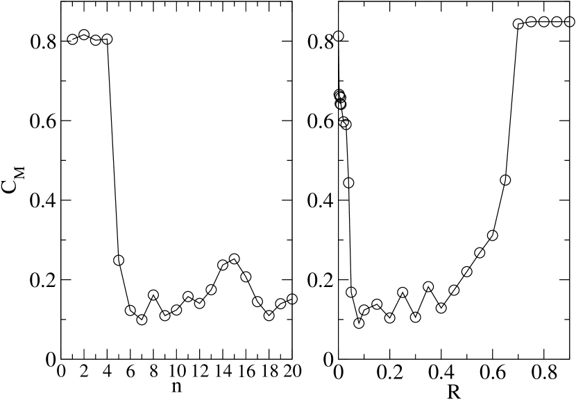
Figure 1: Left: $C_{M}$ vs $n$ with $R=0.1$. Right: $C_{M}$ vs $R$ for $n=10$. In both plots, $U_{0}=10$, $\sqrt{1+2\frac{U_{0}^{2}}{V_{0}^{2}}}=2\pi$, and the time average is performed over the last $2000$ steps in a numerical simulation running for $5000$ steps with $dt=0.01$.

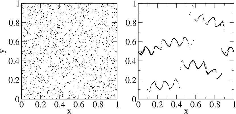
Figure 2: Spatial distribution (statistically stationary) of particles at time $t=0$ (left), and $t=16$ (right panel). Here $R=0.1$, $n=10$, $U_{0}=1$ ($\sqrt{1+2\frac{u_{0}^{2}}{V_{0}^{2}}}=2\pi$, and the initial number of particles $N_{0}=1500$.

where $M$ is the number of boxes in which we divide the system, and $m_{i}$ is the number of particles in box $i$. One has that $0\leq S_{M}\leq\ln M$, such that $S_{M}=0$ is obtained when all the particles are in just one of the boxes, and the $\ln M$ value is reached when $m_{i}=N/M$ for all $i$ (Poisson distribution of particles), i.e., $S_{M}$ decreases when the clustering increases. We define the clustering coefficient as $C_{M}=\exp(<H_{M}>_{t})/M$, where $<.>_{t}$ denotes a temporal average at long times, so that when there is no clustering $C_{M}\approx 1$. In the left panel of fig. (1) we fix $R=0.1$ (much smaller than the system size $L=1$) and plot $C_{M}$ vs $n$ observing that the transition to clustering is obtained for $n\approx 5$, fitting perfectly (7). In the right panel we take $n=10$ and plot $C_{M}$ vs $R$ observing the two transitions indicated in (7). In figure 2 we plot the spatial distribution of particles (in the left panel we plot the initial distribution) in the regime of clustering at time $t=16$ (right) for $R=0.1$ and $n=10$. Here one sees that the particles tend to aggrupate following the sinusoidal flow.

Similar results are obtained for other shear flows. E.g., for the linear shear given by $v(x)=\Gamma x$ if $x\in[0,1/2]$ and $v(x)=\Gamma(1-x)$ for $x\in[1/2,1]$, $\lambda$ is $1/\sqrt{12}$ so that altering the features of the external flow (the values of $\Gamma$) the aggregation properties of the system for fixed $R$ are not changed. However, transitions between non-clustering and clustering distributions are observed by varying $R$.

In the next section we explain analytically the transition to clustering observed in the numerics. This is done by deriving the density evolution equation for the system of particles.

III Continuum description in terms of the density of particles. Linear stability analysis

A continuum theory can give further insight on the model. The process to obtain it is standard Dean , and we just present here a sketch: define the particle density as $\rho({\bf x},t)=\sum_{i=1}^{N}\rho_{i}({\bf x},t)=\sum_{i=1}^{N}\delta({\bf x}_{i}(t)-{\bf x})$, then use an arbitrary function $f({\bf x})$ defined on the coordinate space, and take the time derivative on both sides of the obvious relation $f({\bf x}_{i}(t))=\int d{\bf x}\ \rho_{i}({\bf x},t)f({\bf x})$. Finally, using $\int_{|{\bf x}-{\bf x}_{i}(t)|\leq R}d{\bf x}\ \rho({\bf x},t)=N_{R}(i)$ one arrives to

$$\partial_{t}\rho({\bf x},t)+\nabla_{{\bf x}}\cdot\left[\frac{\rho({\bf x},t)\int_{|{\bf r}-{\bf x}|\leq R}d{\bf r}\ {\bf v}({\bf r},t)\ \rho({\bf r},t)}{\int_{|{\bf r}-{\bf x}|\leq R}d{\bf r}\ \rho({\bf r},t)}\right]=0.$$ (9)

Note that we have maintained the time dependence of the velocity field to reflect the generality of the approach. Eq. (9) can be simply read as that the density of particles is driven by the effective velocity ${\bf v}^{eff}({\bf x},t)=\int_{|{\bf r}-{\bf x}|\leq R}d{\bf r}\ {\bf v}({\bf r},t)\ \rho({\bf r},t)/\int_{|{\bf r}-{\bf x}|\leq R}d{\bf r}\ \rho({\bf r},t)$, whose dependence on the density reveals the self-consistent character of the model. Note also the two trivial limits: a) $R\to 0$ or passive limit, ${\bf v}^{eff}({\bf x},t)\to{\bf v}({\bf x},t)$, and b) $R\to 1$ ($L=1$) for which ${\bf v}^{eff}({\bf x},t)\to 1/N\int d{\bf r}\rho({\bf r},t){\bf v}({\bf r},t)$, i.e., the average velocity of the system of particles, which is the same for all of them (and constant for a time-independent velocity field).

Next we make a linear stability analysis of the stationary homogenous solution, $\rho_{0}$, of eq. (9). We first write $\rho({\bf x},t)=\rho_{0}+\epsilon\psi({\bf x},t)$ where $\epsilon$ is a small parameter, and $\psi({\bf x},t)$ the space-time dependent perturbation, and substitute it in eq. (9). To first order in $\epsilon$, using incompressibility of the flow and denoting $\int_{B}.=\int_{|{\bf r}-{\bf x}|\leq R}.$ we obtain

$$\partial_{t}\psi+\frac{1}{\pi R^{2}}{\bf g}({\bf x})\cdot\nabla_{{\bf x}}\psi+\frac{1}{\pi R^{2}}\nabla_{{\bf x}}\cdot\int_{B}d{\bf r}\ {\bf v}({\bf r},t)\psi({\bf r},t)$$

$$-\frac{1}{(\pi R^{2})^{2}}{\bf g}({\bf x})\cdot\int_{B}d{\bf r}\ \psi({\bf r},t)=0,$$ (10)

with ${\bf g}({\bf x})=\int_{B}d{\bf r}\ {\bf v}({\bf r},t)$. Though linear, the above expression is still rather complicated since it is non-local in space. For the sinusoidal shear flow (taking for simplicity and without lost of generality $U_{0}=0$), we have that ${\bf g}({\bf x})=\hat{\bf y}2\pi R/\omega\sin(\omega x)J_{1}(\omega R)$ with $\hat{\bf y}$ a unitary vector in the $y$ direction, and $J_{1}$ the first order Bessel function, so that eq. (10) becomes

$$\partial_{t}\psi+\frac{2V_{0}J_{1}(\omega R)}{\omega R}\sin(\omega x)\partial_{y}\psi$$

$$+\frac{V_{0}}{\pi R^{2}}\partial_{y}[\int_{B}d{\bf r}\ \sin(\omega r_{x})\psi(r_{x},r_{y},t)]$$

$$-\frac{2V_{0}J_{1}(\omega R)}{\pi\omega R^{3}}\sin(\omega x)\partial_{y}[\int_{B}d{\bf r}\ \psi({\bf r},t)]=0,$$ (11)

where ${\bf r}=(r_{x},r_{y})$.

We are mainly interested in the clustering transition driven by the relative values of $\lambda$ and $R$, so that we next consider the limit $R<<1$. It is very important to note that, to be the expansion in $R$ consistent, all length-scales of the system must also be very small compared with the system size. Specifically, $\lambda=1/\omega<<1$, so that in particular, one cannot expand the $\sin(\omega r_{x})$ in the integrand in eq. (11). Let us detail the calculations. The two integrals appearing in eq. (11) have the approximations (for simplicity of notation we skip the time dependence):

$$I_{a}=\int_{B}d{\bf r}\psi(r_{x},r_{y})=\int_{|{\bf r}^{\prime}|\leq R}d{\bf r}^{\prime}\psi(r_{x}^{\prime}+x,r_{y}^{\prime}+y)$$

$$\approx\int_{|{\bf r}^{\prime}|\leq R}d{\bf r}^{\prime}[\psi(x,y)+r_{x}^{\prime}\partial_{y}\psi(x,y)+r_{y}^{\prime}\partial_{y}\psi(x,y)]$$

$$=\pi R^{2}\psi(x,y)+\Theta(R^{4});$$ (12)

$$I_{b}=\int_{B}d{\bf r}\sin(\omega r_{x})\psi(r_{x},r_{y})$$

$$=\int_{|{\bf r}^{\prime}|\leq R}d{\bf r}^{\prime}\sin(\omega r_{x}^{\prime}+\omega x)\psi(r_{x}^{\prime}+x,r_{y}^{\prime}+y)$$

$$\approx\int_{|{\bf r}^{\prime}|\leq R}\sin(\omega r_{x}^{\prime}+\omega x)[\psi(x,y)+r_{x}^{\prime}\partial_{y}\psi+r_{y}^{\prime}\partial_{y}\psi]$$

$$=\frac{2\pi J_{1}(\omega R)R}{\omega}\sin(\omega x)\psi+\frac{4\pi R^{2}J_{2}(\omega R)}{\omega}\cos(\omega x)\partial_{x}\psi+\Theta(R^{4}).$$

(13)

Here $\Theta(R^{4})$ indicates terms of order $R^{4}$ and superior. After substituting expressions (12)-(13) in eq. (11) the evolution of the perturbation in the small $R$ limit (or better, when the typical length scales of the problem are small) is finally given by

$$\partial_{t}\psi+\frac{2V_{0}J_{1}(\omega R)}{\omega R}\sin(\omega x)\partial_{y}\psi+\frac{4V_{0}J_{2}(\omega R)}{\omega}\cos(\omega x)\partial_{xy}^{2}\psi=0,$$ (14)

where we have neglected terms of order $R$.

Two fundamental features further simplifies the analysis: a) the coefficients are periodic in the spatial coordinates so that Floquet theory can be applied, and b) the coefficients are independent of the $y$ coordinates so that plane waves are solutions on the $y$ direction. Therefore we make the ansatz:

$$\psi(x,y,t)=e^{\Lambda t+i\hat{\omega}y+iKx}\sum_{m=-\infty}^{\infty}\phi_{m}e^{i\omega xm},$$ (15)

where, because of periodic boundary conditions, $\hat{\omega}=2\pi p$ ($p=1,2,...$), $K=2\pi p$ ($p=1,2,...$), and $\phi_{m}$ are complex coefficients. $K$ is restricted to the first Brillouin zone determined by $-\omega/2\leq K\leq\omega/2$, and $\hat{\omega}$ is not bounded.

If any of the eigenvalues $\Lambda$ is positive then the perturbation grows (the homogenous solution is unstable) and clustering emerges in the system. Thus we look for the conditions to have $\Lambda>0$. Using the exponential formula for the sine and cosine functions, and substituting expression (15) in eq. (14) we obtain, after grouping the terms with the same exponential argument,

$$\Lambda_{m}\phi_{m}+\phi_{m-1}[\alpha_{1}-\beta m]+\phi_{m+1}[\alpha_{2}-\beta m]=0,$$ (16)

with $\alpha_{1}=a_{1}\hat{\omega}/2-a_{2}\hat{\omega}K/2+a_{2}\omega\hat{\omega}/2$, $\alpha_{2}=-a_{1}\hat{\omega}/2-a_{2}\hat{\omega}K/2-a_{2}\omega\hat{\omega}/2$, and $\beta=a_{2}\omega\hat{\omega}/2$, with the notations $a_{1}=2V_{0}J_{1}(\omega R)/(\omega R)$ and $a_{2}=4V_{0}J_{2}(\omega R)/\omega$.

For a simple theoretical analysis we just consider the three Fourier modes $m=0,\pm 1$ and neglect the rest. Diagonalizing the corresponding $3\times 3$ matrix of coefficients of the system in eq. (16) we obtain three eigevanlues, one zero and the other two given by

$$\Lambda_{\pm}(K)=\pm\frac{V_{0}\hat{\omega}}{\omega R}\sqrt{8J_{2}^{2}K^{2}R^{2}-4\omega RJ_{2}J_{1}-2J_{1}^{2}},$$ (17)

where the Bessel functions, $J_{1}$ and $J_{2}$, are evaluated at $\omega R$. The expression for $\Lambda_{+}$ is cuadratic in $K$ with a positive coefficient for the term in $K^{2}$, so that taking into account that $-\omega/2\leq K\leq\omega/2$, the inestability is obtained when $\Lambda_{+}(K=\omega/2)$ is positive, i.e.,

$$J_{2}(\omega R)^{2}\omega^{2}R^{2}-2\omega RJ_{2}(\omega R)J_{1}(\omega R)-J_{1}(\omega R)^{2}\geq 0.$$ (18)

Numerically one solves the above inequality and obtains that the condition for instability is $\omega R\geq 2.5$, which, despite the many approximations made to derive it, fits well with the numerical result $1/\omega\leq 2R$ (eq. (7) for $U_{0}=0$). We have checked that the above result is improved by including more modes in the Floquet analysis. In particular, considering $m=0,\pm 1,\pm 2$, the final condition for the maximum exponent to be positive is $\omega R\geq 1.32$. We believe that in the limit $m\to\infty$ the numerical result is approached. Therefore this analysis confirms that the derived continuum description eq. (9) properly describes the discrete interacting particles model, and that the clustering emerges as a deterministic instability of the density equation.

IV Summary

In this work we have proposed a very simple model for an ensemble of particles self-consistently driven by an external shear flow. Despite its simplicity the model shows a very interesting behavior where a transition to grouping of particles are observed. An hypothesis for the appearence of the clustering has been presented. It esentially says that the clustering appears when the length scale that comes from the comparison of the shear flow and the velocity field amplitudes is smaller than the typical interaction radius of the particles. This hypothesis has been numerically checked and also a continuum description has been derived that confirms it.

A more realistic interaction of the particles, for example decaying with the distance within $R$, is planned to be studied in the future. Also, it will be interesting a detailed study of the role of a noise term in the dynamics of the particles (which in the continuum description is a difussion term), and the analysis when a chaotic flow is considered.

V Acknowledgments

I have benefited from many useful conversations with Emilio Hernández-García. I also acknowledge discussions with Damià Gomila and Pere Colet. Work supported from MCyT of Spain under projects REN2001-0802-C02-01/MAR (IMAGEN) and BFM2000-1108 (CONOCE), and from a Ramón y Cajal fellowship of the Spanish MEC.

References

- (1) J. M. Ottino, The Kinematics of Mixing: Stretching, Chaos and Transport (Cambridge Univ. Press, Cambridge, 1989); T. Bohr, M. Jensen, G. Paladin, and A. Vulpiani, Dynamical Systems Approach to Turbulence (Cambridge University Press, Cambridge, 1998); Focus issue on Activity in Chaotic Flows [Chaos 12, 372 (2002)].
- (2) D. del-Castillo-Negrete, CHAOS 10, 75 (2000).
- (3) G. Falkovich, K. Gawedzki, M. Vergassola, Rev. Mod. Phys. 73, 913 (2001).
- (4) A. Celani, M. Cencini, A. Mazzino, and M. Vergassola, Phys. Rev. Lett. 89, 234502 (2002).
- (5) G. Boffetta, D. del-Castillo-Negrete, C. López, G. Pucacco, and A. Vulpiani, Phys. Rev. E 67, 026224 (2003).
- (6) D. del-Castillo-Negrete, and M.C. Firpo, CHAOS 12, 496 (2002); D. del-Castillo-Negrete, In Dynamics and Thermodynamics of Systems with Long Range Interactions, Edited by T. Dauxois et al. Lecture Notes in Physics Vol. 602, Springer, 2002.
- (7) G. Flierl, D. Grunbaum, s. Levin, and D. Olson, J. Theor. Biol. 196, 397 (1999); T. Vicsek et al., Phys. Rev. Lett. 75, 1226 (1995); D. Helbing, Rev. Mod. Phys. 73, 1067 (2001).
- (8) A. Puglisi, V. Loreto, U. Marini Bettolo Marconi, and A. Vulpiani Phys. Rev. E 59, 5582 (1999)
- (9) D. S. Dean, J. Phys. A 29, L613 (1996); U. M.B. Marconi and P. Tarazona, J. Chem. Phys. 110, 8032 (1999).