Nonlinear Lattice Dynamics of Bose-Einstein Condensates

Abstract

The Fermi-Pasta-Ulam (FPU) model, which was proposed 50 years ago to examine thermalization in non-metallic solids and develop “experimental” techniques for studying nonlinear problems, continues to yield a wealth of results in the theory and applications of nonlinear Hamiltonian systems with many degrees of freedom. Inspired by the studies of this seminal model, solitary-wave dynamics in lattice dynamical systems have proven vitally important in a diverse range of physical problems—including energy relaxation in solids, denaturation of the DNA double strand, self-trapping of light in arrays of optical waveguides, and Bose-Einstein condensates (BECs) in optical lattices. BECS, in particular, due to their widely ranging and easily manipulated dynamical apparatuses—with one to three spatial dimensions, positive-to-negative tuning of the nonlinearity, one to multiple components, and numerous experimentally accessible external trapping potentials—provide one of the most fertile grounds for the analysis of solitary waves and their interactions. In this paper, we review recent research on BECs in the presence of deep periodic potentials, which can be reduced to nonlinear chains in appropriate circumstances. These reductions, in turn, exhibit many of the remarkable nonlinear structures (including solitons, intrinsic localized modes, and vortices) that lie at the heart of the nonlinear science research seeded by the FPU paradigm.

The Fermi-Pasta-Ulam (FPU) model was formulated in 1954 in an attempt to explain heat conduction in non-metallic lattices and develop “experimental” (computational) methods for research on nonlinear dynamical systems Weissert (1997). Further studies of this problem ten years later led to the first analytical description of solitons (using the Korteweg-de Vries equation, which is a continuum approximation of the discrete FPU system), which have since become one of the most fundamental paradigms of nonlinear science. These nonlinear waves occur ubiquitously in rather diverse physical situations ranging from water waves to plasmas, optical fibers, superconductors (long Josephson junctions), quantum field theories, and more. Over the past several years, the study of solitons and coherent structures in Bose-Einstein condensates (BECs) has come to the forefront of experimental and theoretical efforts in soft condensed matter physics, drawing the attention of atomic and nonlinear physicists alike. Observed experimentally for the first time in 1995 in vapors of sodium and rubidium Davis et al. (1995); Anderson et al. (1995), a BEC—a macroscopic cloud of coherent quantum matter—is attained when ($10^{3}$ to $10^{6}$) atoms, confined in magnetic traps, are optically and evaporatively cooled to a fraction of a microkelvin. The macroscopic behavior of BECs near zero temperature is modeled very well by the Gross-Pitaevskii equation (a time-dependent nonlinear Schrödinger equation with an external potential), which admits a wide range of coherent structure solutions. Especially attractive is that experimentalists can now engineer a wide variety of external trapping potentials (of either magnetic or optical origin) confining the condensate. As a key example, we focus on BECs loaded into deep, spatially periodic optical potentials, effectively splitting the condensate into a chain of linearly-interacting, nonlinear droplets, the dynamics of which is accurately characterized by nonlinear lattice models. This paper highlights some of the quasi-discrete nonlinear dynamical structures in BECs reminiscent of the discoveries that originated from the FPU model.

I Introduction

One of the most important nonlinear problems, whose origin dates back to the early 20th century, concerns the conduction of heat in dielectric crystals. As early as 1914, Peter Debye suggested that the finite thermal conductivity of such lattices is due to the nonlinear interactions among lattice vibrations (i.e., phonon-phonon scattering) Zabusky (1984). To understand the process of thermalization—which refers to how and to what extent energy is transported from coherent modes and macroscopic scales to internal, microscopic ones Friesecke and Pego (1999)—and to develop computational techniques for studying nonlinear dynamical systems, Fermi, Pasta, and Ulam (FPU) posed the following question in 1954: How long does it take for long-wavelength oscillations to transfer their energy into an equilibrium distribution in a one-dimensional string of nonlinearly interacting particles? This question has since spawned a diverse array of activities attempting to answer it and fomented a strong impetus to research in topics such as soliton theory, discrete lattice dynamics, and KAM theory. Furthermore, these fronts remain active research topics Friesecke and Pego (1999, 2002, 2004a, 2004b); Lepri et al. (2003).

Before the FPU work, it was commonly assumed that high-dimensional Hamiltonian systems behave ergodically in the sense that a smooth initial energy distribution should quickly relax until it is ultimately distributed evenly among all of the system’s modes (that is, thermalization should occur). To explicitly verify this fundamental hypothesis of statistical physics, FPU constructed a one-dimensional dynamical lattice, with $N$ identical particles which interact according to an anharmonic repulsive force.

Running numerical simulations on the computers available in the early fifties, FPU observed that the lattice did not relax to thermal equilibrium, contrary to everybody’s expectations Fermi et al. (1955); Zabusky (1984); Lichtenberg and Lieberman (1992); Ablowitz and Clarkson (1991); Weissert (1997). An especially striking observation was a beating effect, in the form of a near-recurrence of the initial long-scale configuration, which reappeared after a large number of oscillations involving short-scale modes. In this manner, more than $97\%$ of the energy returned to the initial mode. Moreover, this finding was robust with respect to variations in the total number of particles and particular choice of the (power-law) anharmonicity in the interaction between them.

Motivated by this study, Zabusky and Kruskal considered a continuum version of the model, showing that the dynamics of small-amplitude, long-wavelength perturbations obeys [on the timescale $\sim$ $($wavelength$)^{3}$] the Korteweg-de Vries (KdV) equation. They subsequently introduced the concept of solitons (solitary waves) in terms of the KdV equation Ablowitz and Clarkson (1991); Zabusky and Kruskal (1965); Zabusky (1984). The explanation for the lack of thermalization is that the energy gets concentrated in robust coherent structures (the solitons), which interact elastically and thus do not transfer their energy into linear lattice modes (phonon waves, also referred to as “radiation”) Friesecke and Pego (1999). The KdV equation thereby became the first example in the celebrated class of nonlinear partial differential equations (PDEs) that are integrable by means of the inverse scattering transform. It was later followed by numerous other important PDEs, such as the nonlinear Schrödinger equation, the sine-Gordon equation, higher dimensional examples (including the Kadomtsev-Petviashvili and the Davey-Stewartson equations) and multi-component examples (including the Manakov equation) Dodd et al. (1982); Drazin and Johnson (1989).

Since then, the study of solitons, and more general coherent structures, has become one of the paradigms of nonlinear science Whitham (1974); Ablowitz and Clarkson (1991); Ablowitz and Segur (1981). Such dynamical behavior occurs in a wide variety of physical systems—including (to name just a few examples) nonlinear optics, fluid mechanics, plasma physics, and quantum field theory. Over the past several years, the impact of solitary-wave dynamics has been especially significant in the study of Bose-Einstein condensates (BECs) Pethick and Smith (2002); Dalfovo et al. (1999). In this short review, we focus on this application and, in particular, its description in physically appropriate cases in terms of dynamical lattices.

The rest of this paper is organized as follows. In Section II, we define the FPU problem and briefly survey its mathematical properties. In Section III, we provide an introduction to Bose-Einstein condensates and their solitary wave solutions. We consider, in particular, BECs loaded into optical lattices (OLs), and use a Wannier-function expansion to derive a dynamical lattice model describing this system. In appropriate limits, this leads to a (generally, multiple-component) discrete nonlinear Schrödinger (DNLS) equation Alfimov et al. (2002a). In Section IV, we examine the regime in which a deep, spatially periodic OL potential effectively fragments the BEC into a chain of weakly interacting droplets. The resulting model, which consists of a Toda lattice with on-site potentials, produces self-localized modes that may be construed as solitons of the underlying BEC. Section V concludes the paper, discussing a number of future directions.

II The FPU Problem

The FPU model consists of a chain of particles connected by nonlinear springs. The constitutive law of the model, i.e., the relation between the interaction force $F$ and the distance $y$ between adjacent atoms in the chain (with only nearest-neighbor interactions postulated), was taken to be $F(y)=-[y+G(y)]$. FPU considered three different functional forms of $G(y)$: quadratic, cubic, and piecewise linear Fermi et al. (1955).

In the case of a cubic force law Lichtenberg and Lieberman (1992), $F(y)=-(y+3\beta y^{3})$, where $\beta$ is an effective anharmonicity coefficient, one may write

$$\begin{array}[]{rcl}\displaystyle\ddot{y}_{j}&=&\displaystyle\frac{y_{j+1}-2y_{j}+y_{j-1}}{h^{2}}\left\{1+\frac{\beta}{h^{2}}\left[(y_{j+1}-y_{j})^{2}\right.\right.\\[8.61108pt] &+&\displaystyle\left.\left.(y_{j}-y_{j-1})^{2}+(y_{j+1}-y_{j})(y_{j}-y_{j-1})\right]\vphantom{\frac{\beta}{h^{2}}}\right\}\,,\end{array}~{}$$ (1)

which is supplemented with fixed boundary conditions, $y_{0}=y_{N}=0$. FPU Fermi et al. (1955); Ablowitz and Clarkson (1991) used the initial condition $y_{j}(0)=\sin(j\pi/N)$ and $\dot{y}_{j}(0)=0$. This form (1) of the FPU chain is obtained by discretizing the continuous nonlinear string,

$$\frac{\partial^{2}y}{\partial t^{2}}-\frac{\partial^{2}y}{\partial x^{2}}\left[1+3\beta\left(\frac{\partial y}{\partial x}\right)^{\!2}\right]=0$$ (2)

with the following approximations to the continuum derivatives:

$$\begin{array}[]{rcl}\displaystyle\frac{\partial y}{\partial x}&\equiv&\displaystyle\left\{\frac{y_{j+1}-y_{j}}{h}\,,\,\frac{y_{j}-y_{j-1}}{h}\right\},\\[10.76385pt] \displaystyle\frac{\partial^{2}y}{\partial x^{2}}&\equiv&\displaystyle\frac{y_{j+1}-2y_{j}+y_{j-1}}{h^{2}}.\end{array}$$ (3)

Here, $y_{j}$ is the displacement of the $j$-th particle from its equilibrium position, $h\equiv L/N$ is the normalized spacing (the distance between the particles), $L$ is the string’s length, and $N$ is the number of particles, which FPU took to be $16$, $32$, or $64$ in their calculations. (Using equation (1), the onset of resonance overlaps was studied in the FPU problem in the first ever application of Chirikov’s overlap criterion Lichtenberg and Lieberman (1992); Izrailev and Chirikov (1966).)

With an appropriate scaling ($t\rightarrow ht$, $y\rightarrow hy\sqrt{3/\beta}$), the FPU chain can also be written

$$\ddot{y}_{j} =(y_{j+1}-y_{j})-(y_{j}-y_{j-1})$$

$$\quad+\frac{1}{3}\left[(y_{j+1}-y_{j})^{3}-(y_{j}-y_{j-1})^{3}\right]\,.$$ (4)

Using the continuum field variable $u$ Driscoll and O’Neil (1976),

$$u\equiv-\frac{y_{t}}{2h}+\frac{1}{2}\int_{0}^{y_{x}}(1+h^{2}\eta^{2})^{1/2}d\eta,$$ (5)

Eq. (2) yields, to lowest order in $h$, the modified Korteweg-de Vries (mKdV) equation (with $\tau\equiv h^{3}t/24$, $\xi\equiv x-ht$),

$$u_{\tau}+12u^{2}u_{\xi}+u_{\xi\xi\xi}=0\,,$$ (6)

which is further reduced to the KdV equation proper via the Miura transformation Zabusky (1984); Ablowitz and Clarkson (1991); Whitham (1974); Ablowitz and Segur (1981).

One can also derive the KdV equation directly from an FPU chain with a quadratic anharmonicity in the inter-particle interaction Ablowitz and Clarkson (1991); Fermi et al. (1955); Zabusky and Kruskal (1965), $F(y)=-(y+\alpha y^{2})$. In the latter case, the discrete FPU model takes the form

$$\ddot{y}_{j}=\frac{y_{j+1}-2y_{j}+y_{j-1}}{h^{2}}\left(1+\alpha\frac{y_{j+1}-y_{j-1}}{h}\right)\,.$$ (7)

To study the near-recurrence phenomenon in Eq. (7), Zabusky and Kruskal Zabusky and Kruskal (1965); Zabusky (1984) derived its continuum limit ($h\longrightarrow 0$, $Nh\longrightarrow 1$),

$$y_{tt}=y_{xx}+\varepsilon y_{x}y_{xx}+\frac{1}{12}h^{2}y_{xxxx}+O(\varepsilon h^{2},h^{4})\,,$$ (8)

where $\varepsilon\equiv 2\alpha h$.

Unidirectional asymptotic solutions to Eq. (8) are constructed with Ablowitz and Clarkson (1991)

$$y\sim\phi(\xi,\tau)\,,\quad\xi\equiv x-t\,,\quad\tau\equiv\frac{1}{2}\varepsilon t,$$ (9)

where the function $\phi$ obeys the equation

$$\phi_{\xi\tau}+\phi_{\xi}\phi_{\xi\xi}+\delta^{2}\phi_{\xi\xi\xi\xi}+O\left(h^{2},h^{4}\varepsilon^{-1}\right)\,=0\,,$$ (10)

for small $\delta^{2}\equiv h^{2}\varepsilon^{-1}/12$. Finally, with $u\equiv\phi_{\xi}$, one obtains the KdV equation from Eq. (10) Kruskal (1975):

$$u_{\tau}+uu_{\xi}+\delta^{2}u_{\xi\xi\xi}\,=0\,.$$ (11)

Eq. (11) has solitary-wave solutions of the form

$$u(x,t)=2\kappa^{2}\mbox{sech}^{2}\left[\kappa(x-4\kappa^{2}t-x_{0})\right]\,,$$ (12)

with constants $\kappa$ and $x_{0}$. [Note that a more rigorous derivation of the KdV equation from the FPU chain (as a fixed point of a renormalization process) has recently been developed Friesecke and Pego (1999).]

Although the solitary-pulse solution (12) has been well-known since the original paper by Korteweg and de Vries, it was the paper by Zabusky and Kruskal Zabusky and Kruskal (1965) that revealed the particle-like behavior of the pulses in numerical simulations. (The term “soliton” was coined in that paper to describe them.) Since then, solitons have become ubiquitous, as their study has yielded vital insights into numerous physical problems Whitham (1974); Ablowitz and Clarkson (1991); Ablowitz and Segur (1981); Newell (1974); Drazin and Johnson (1989); Dodd et al. (1982). In the next section, we discuss their importance to Bose-Einstein condensation Dalfovo et al. (1999); Pethick and Smith (2002).

It is remarkable that even today, 50 years from the original derivation Fermi et al. (1955), FPU chains are themselves still studied as a means of understanding a variety of nonlinear phenomena. Recent studies focus not only on the model’s solitary-wave solutions and their stability Friesecke and Pego (1999, 2002, 2004a, 2004b); Rink (2002), but also on its thermodynamic properties and connections with the Fourier law of heat conductivity Lepri et al. (2003), its dynamical systems/invariant manifold aspects Rink (2003, 2001), and its connections with weak turbulence theory Biello et al. (2002).

To conclude this section, we remark that the most natural discrete model that has been derived from the NLS (or GP) equation for a soliton train is the Toda lattice Gerdjikov et al. (1996) (see also the details discussed below). However, the leading-order nonlinear truncation of the latter lattice equation once again yields the FPU model. Conversely, one can approximate the FPU chain by the NLS equation in the high-frequency limit Berman and Kolovskii (1984); Lichtenberg and Lieberman (1992). The validity of this approximation varies with time due to energy exchange between modes.

III Bose-Einstein Condensation

At low temperatures, bosonic particles in a dilute gas can reside in the same quantum (ground) state, forming a Bose-Einstein condensate (BEC) Pethick and Smith (2002); Dalfovo et al. (1999); Ketterle (1999); Burnett et al. (1999). Seventy years after they were first predicted theoretically, BECs were finally observed experimentally in 1995 in vapors of rubidium and sodium Anderson et al. (1995); Davis et al. (1995). In these experiments, atoms were loaded into magnetic traps and evaporatively cooled to temperatures on the order of a fraction of a microkelvin. To record the properties of the BEC, the confining trap was then switched off, and the expanding gas was optically imaged Dalfovo et al. (1999). A sharp peak in the velocity distribution was observed below a critical temperature, indicating that condensation had occurred.

Under experimental conditions, BECs are inhomogeneous, so condensation can be observed in both momentum and coordinate space. The number of condensed atoms $\mathcal{N}$ ranges from several thousand (or less) to several million (or more). The magnetic traps confining BECs are usually well-approximated by harmonic potentials. There are two characteristic length scales. One is the harmonic oscillator length, $a_{\mathrm{ho}}=\sqrt{\hbar/(m\omega_{\mathrm{ho}})}$ (which is, typically, on the order of a few microns), where $m$ is the atomic mass and $\omega_{\mathrm{ho}}=(\omega_{x}\omega_{y}\omega_{z})^{1/3}$ is the geometric mean of the trapping frequencies. The second scale is the mean healing length, $\chi=1/\sqrt{8\pi|a|\bar{n}}$, where $\bar{n}$ is the mean density of the atoms, and $a$, the (two-body) $s$-wave scattering length, is determined by collisions between atoms Pethick and Smith (2002); Dalfovo et al. (1999); Köhler (2002); Baizakov et al. (2002). Interactions between atoms are repulsive when $a>0$ and attractive when $a<0$. The length scales in BECs should be compared to those in condensed media like superfluid helium, in which the effects of inhomogeneity occur on a microscopic scale fixed by the interatomic distance Dalfovo et al. (1999).

With two-body collisions described in the mean-field approximation, a dilute Bose-Einstein gas is very accurately modeled by the cubic nonlinear Schrödinger equation (NLS) with an external potential [i.e., by the so-called Gross-Pitaevskii (GP) equation]. An important case is that of cigar-shaped BECs, which are tightly confined in two transverse directions (with the radius on the order of the healing length) and quasi-free in the longitudinal dimension Salasnich et al. (2002a); Pérez-García et al. (1998); Salasnich et al. (2002b); Band et al. (2003); Lieb et al. (2003). In this regime, one employs the 1D limit of the 3D mean-field theory, generated by averaging in the transverse plane (rather than the 1D mean-field theory per se, which would be appropriate were the transverse dimension on the order of the atomic size Salasnich et al. (2002a); Pérez-García et al. (1998); Salasnich et al. (2002b); Band et al. (2003); Lieb et al. (2003)).

The original GP equation, describing the BEC near zero temperature, is Gross (1961); Pitaevskii (1961); Dalfovo et al. (1999); Köhler (2002); Baizakov et al. (2002)

$$i\hbar{\Psi}_{t}=\left(-\frac{\hbar^{2}\nabla^{2}}{2m}+g_{0}|\Psi|^{2}+{\mathcal{V}}(\vec{r})\right)\Psi,$$ (13)

where $\Psi=\Psi(\vec{r},t)$ is the condensate wave function normalized to the number of atoms $\mathcal{N}$, ${\mathcal{V}}(\vec{r})$ is the external potential, and the effective interaction constant is Dalfovo et al. (1999) $g_{0}=[4\pi\hbar^{2}a/m][1+O(\zeta^{2})]$, where $\zeta\equiv\sqrt{|\Psi|^{2}|a|^{3}}$ is the dilute-gas parameter. The resulting normalized form of the 1D equation is Salasnich et al. (2002a); Pérez-García et al. (1998); Salasnich et al. (2002b); Band et al. (2003); Lieb et al. (2003)

$$i\psi_{t}=-\frac{1}{2}\psi_{xx}+g|\psi|^{2}\psi+V(x)\psi,$$ (14)

where $\psi$ and $V$ are, respectively, the rescaled 1D wave function (a result of averaging in the transverse directions) and external potential. The rescaled self-interaction parameter $g$ is tunable (even its sign), because the scattering length $a$ can be adjusted using magnetic fields in the vicinity of a Feshbach resonance Donley et al. (2001); Kevrekidis et al. (2003a).

III.1 BECs in Optical Lattices and Superlattices

BECs can be loaded into optical lattices (or superlattices, which are small-scale lattices subjected to a long-scale periodic modulation), which are created experimentally as interference patterns of counter-propagating laser beams Anderson and Kasevich (1998a); Jona-Lasinio et al. (2003); Konotop et al. ; Orzel et al. (2001a); Morsch et al. (2001a); Cataliotti et al. (2001); Greiner et al. (2001); Greiner et al. (2002a). Over the past several years, a vast research literature has developed concerning BECs in such potentials Anderson and Kasevich (1998b); Greiner et al. (2002b); Burger et al. (2001); Morsch et al. (2001b); Choi and Niu (1999); Jaksch et al. (1998); Peil et al. (2003); Rey et al. (2003); Porter and Cvitanović (2004a); Porter and Kevrekidis (2004); Bronski et al. (2001a); Kevrekidis et al. (2003b, c, d), as they are of considerable interest both experimentally and theoretically. Among other phenomena, they have been used to study Josephson effects Anderson and Kasevich (1998b), squeezed states Orzel et al. (2001b), Landau-Zener tunneling and Bloch oscillations Morsch et al. (2001b), controllable condensate splitting Porter and Kevrekidis (2004), and the transition between superfluidity and Mott insulation at both the classical Smerzi et al. (2002); Cataliotti et al. (2003) and quantum Greiner et al. (2002b) levels. Moreover, with each lattice site occupied by one alkali atom in its ground state, BECs in optical lattices show promise as a register in a quantum computer Porto et al. (2003); Vollbrecht et al. (2004).

With the periodic potential $V(x)=V(x+L)$, one may examine stationary solutions to (14) in the form

$$\psi(x,t)=R(x)\exp\left(i\left[\theta(x)-\mu t\right]\right)\,,$$ (15)

where $\mu$, the BEC’s chemical potential, is determined by the number of atoms in the BEC; it is positive for repulsive BECs and can assume either sign for attractive BECs. Using the relation $d\theta/dx=c/R^{2}$ (“angular momentum” conservation), one derives a parametrically forced Duffing-oscillator equation for the amplitude function Porter and Cvitanović (2004a); Porter and Cvitanović (2004b); Bronski et al. (2001a, b, c); Alfimov et al. (2002b),

$$R^{\prime\prime}-\frac{c^{2}}{R^{3}}+\mu R-gR^{3}-V(x)R=0\,,$$ (16)

where $R^{\prime\prime}\equiv d^{2}R/dx^{2}$.

Equation (16) admits both localized and spatially extended solutions. Supplemented with appropriate boundary conditions, it yields both bright and dark solitons, which correspond, respectively, to localized humps on the zero background, and localized dips in a finite-density background. These states are similar to the bright and dark solitons in nonlinear optics; they are stable, respectively, in attractive and repulsive 1D BECs Alfimov et al. (2002b); Louis et al. (2003).

When $V(x)$ is spatially periodic, the bright solitons resemble gap solitons, which are supported by Bragg gratings in nonlinear optical systems. In BECs, they have been observed in two situations: (1) the small-amplitude limit, with the value of $\mu$ close to forbidden zones (“gaps”) of the underlying linear Schrödinger equation with a periodic potential Konotop and Salerno (2002); Sakaguchi and Malomed (2004); and (2) in the tight-binding approximation (discussed below), for which the continuous NLS equation can be replaced by its discrete counterpart—the so-called discrete nonlinear Schrödinger (DNLS) equation Abdullaev et al. (2001). In the latter context, the strongly localized solutions are known as intrinsic localized modes (ILMs) or discrete breathers. Spatially extended wave functions with periodic or quasi-periodic $R(x)$, which may be either resonant or non-resonant with respect to the periodic potential $V(x)$, are known as modulated amplitude waves and have been shown to be stable (against arbitrary small perturbations) in some cases Bronski et al. (2001a, b, c); Porter and Cvitanović (2004a); Porter and Cvitanović (2004b); Porter and Kevrekidis (2004).

III.2 Lattice Dynamics

In the presence of a strong optical lattice, the GP equation (14) can be reduced to the DNLS equation Alfimov et al. (2002a, b); Kevrekidis and Frantzeskakis (2004). To justify this approximation, the wave function is expanded in terms of a set of Wannier functions localized near the minima of the potential wells.

The eigenvalue problem associated with the linear part of Eq. (14) is

$$-\varphi_{k,\alpha}^{\prime\prime}+V(x)\varphi_{k,\alpha}=E_{\alpha}(k)\varphi_{k,\alpha}\,,$$ (17)

where $\varphi_{k,\alpha}$ can be expressed in terms of Floquet-Bloch functions, $\varphi_{k,\alpha}=e^{ikx}u_{k,\alpha}(x)$, with $u_{k,\alpha}(x)=u_{k,\alpha}(x+L)$ and $\alpha$ indexing the energy bands, so that $E_{\alpha}(k)=E_{\alpha}(k+[2\pi/L])$ Ashcroft and Mermin (1976). The energy is represented using Fourier series,

$$E_{\alpha}(k)=\sum_{n=-\infty}^{\infty}\hat{\omega}_{n,\alpha}e^{iknL}\,,\quad\hat{\omega}_{n,\alpha}=\hat{\omega}_{-n,\alpha}=\hat{\omega}_{n,\alpha}^{\ast}\,,$$ (18)

where the asterisk denotes complex conjugation and

$$\hat{\omega}_{n,\alpha}=\frac{L}{2\pi}\int_{-\pi/L}^{\pi/L}E_{\alpha}(k)e^{-iknL}dk\,.$$ (19)

Although the Floquet-Bloch functions provide a complete orthonormal basis, it is more convenient to utilize Wannier functions (also indexed by $\alpha$),

$$w_{\alpha}(x-nL)=\sqrt{\frac{L}{2\pi}}\int_{-\pi/L}^{\pi/L}\varphi_{k,\alpha}(x)e^{-inkL}dk\,,$$ (20)

which are centered about $x=nL$ ($n\in\mathbb{Z}$). The Wannier functions constitute a complete orthonormal basis with respect to both $n$ and $\alpha$. One can also guarantee that the Wannier functions are real by conveniently choosing phases of the Floquet-Bloch functions.

Given the orthonormality of the Wannier function basis, any solution of (14) can be expanded in the form

$$\psi(x,t)=\sum_{n,\alpha}c_{n,\alpha}(t)w_{n,\alpha}(x)\,,$$ (21)

with coefficients satisfying a DNLS equation with long-range interactions,

$$\begin{array}[]{rcl}\displaystyle i\frac{dc_{n,\alpha}}{dt}&=&\displaystyle\sum_{n_{1}}c_{n_{1},\alpha}\hat{\omega}_{n-n_{1},\alpha}\\[12.91663pt] &+&\displaystyle g\sum_{\alpha_{1},\alpha_{2},\alpha_{3}}\sum_{n_{1},n_{2},n_{3}}c_{n_{1},\alpha_{1}}^{\ast}c_{n_{2},\alpha_{2}}c_{n_{3},\alpha_{3}}W_{\alpha,\alpha_{1},\alpha_{2},\alpha_{3}}^{n,n_{1},n_{2},n_{3}}\,,\end{array}$$ (22)

as was illustrated in Alfimov et al. (2002a). In (22),

$$W_{\alpha,\alpha_{1},\alpha_{2},\alpha_{3}}^{n,n_{1},n_{2},n_{3}}=\int_{-\infty}^{\infty}w_{n,\alpha}w_{n_{1},\alpha_{1}}w_{n_{2},\alpha_{2}}w_{n_{3},\alpha_{3}}dx\,.$$ (23)

Because the Wannier functions are real, the integral in (23) is symmetric with respect to all permutations of both $(\alpha,\alpha_{1},\alpha_{2},\alpha_{3})$ and $(n,n_{1},n_{2},n_{3})$.

Although Eqs. (22) are intractable as written, several important special cases can be studied Alfimov et al. (2002a). The nearest-neighbor coupling approximation is valid when $|\hat{\omega}_{1,\alpha}|\gg|\hat{\omega}_{n,\alpha}|$ for $n>1$. More generally, one can assume that the Fourier coefficients in (18) decay rapidly beyond a finite number of harmonics. This simplifies the linear term in (22). Additionally, because $w_{n,\alpha}$ is localized about its center at $x=nL$, it is sometimes reasonable to assume that the coefficients satisfying $n=n_{1}=n_{2}=n_{3}$ dominate $W_{\alpha,\alpha_{1},\alpha_{2},\alpha_{3}}^{n,n_{1},n_{2},n_{3}}$, so that the others may be neglected. In the nearest-neighbor regime, this implies that

$$\begin{array}[]{rcl}\displaystyle i\frac{d{c}_{n,\alpha}}{dt}&=&\hat{\omega}_{0,\alpha}c_{n,\alpha}+\hat{\omega}_{1,\alpha}(c_{n-1,\alpha}+c_{n+1,\alpha})\\[8.61108pt] &+&\displaystyle g\sum_{\alpha_{1},\alpha_{2},\alpha_{3}}W_{\alpha,\alpha_{1},\alpha_{2},\alpha_{3}}c_{n,\alpha_{1}}^{\ast}c_{n,\alpha_{2}}c_{n,\alpha_{3}}\,,\end{array}$$ (26)

where $W_{\alpha,\alpha_{1},\alpha_{2},\alpha_{3}}\equiv W_{\alpha,\alpha_{1},\alpha_{2},\alpha_{3}}^{n,n,n,n}$ is independent of $n$. This leads to the tight-binding model,

$$\begin{array}[]{rcl}\displaystyle i\frac{d{c}_{n,\alpha}}{dt}&=&\hat{\omega}_{0,\alpha}c_{n,\alpha}+\hat{\omega}_{1,\alpha}(c_{n-1,\alpha}+c_{n+1,\alpha})\\[8.61108pt] &+&\displaystyle gW_{\alpha,\alpha,\alpha,\alpha}|c_{n,\alpha}|^{2}c_{n,\alpha}\,,\end{array}$$ (27)

in the single-band approximation. Typically, this approximation is valid if the height of the barrier between potential wells is large and if the wells are well-separated. While this intuition may be generally true, the Wannier function reduction provides a systematic tool that can establish the validity of the approximation on a case by case basis (by determining the overlap coefficients); see, e.g., Alfimov et al. (2002a) for specific examples. Including next-nearest-neighbor coupling in this regime allows one to study interactions between intrasite and intersite nonlinearities.

In more general situations in which single-band descriptions are inadequate because of resonant, nonlinearity-induced interband interactions, one can simplify (26) by assuming that $\hat{\omega}_{1,\alpha}\equiv\hat{\omega}_{1,\alpha}(\epsilon)=O(\epsilon)$ as $\epsilon\rightarrow 0$. Applying the phase shift $c_{n,\alpha}(t)=\exp[i\hat{\omega}_{0,\alpha}t]\tilde{c}_{n\alpha}(t)$, so that the nonlinear terms consist of oscillatory exponents, and supposing that $\tilde{c}_{n,\alpha}(0)$ is sufficiently small and may be ignored, we conclude that, on the time scale $\sim 1/\epsilon$, the exponents oscillate rapidly except when $\alpha=\alpha_{2}$, $\alpha_{1}=\alpha_{3}$ or $\alpha=\alpha_{3}$, $\alpha_{1}=\alpha_{2}$. Through time-averaging, one obtains

$$\begin{array}[]{rcl}\displaystyle i\frac{d\tilde{c}_{n,\alpha}}{dt}&=&\hat{\omega}_{1,\alpha}(\tilde{c}_{n-1,\alpha}+\tilde{c}_{n+1,\alpha})\\[8.61108pt] \displaystyle\hfil&+&\displaystyle g\sum_{\alpha_{1}}W_{\alpha,\alpha_{1}}|\tilde{c}_{n,\alpha_{1}}|^{2}\tilde{c}_{n,\alpha_{1}}\,,\end{array}$$ (28)

where $W_{\alpha,\alpha_{1}}\equiv W_{\alpha,\alpha_{1},\alpha,\alpha_{1}}$ describes the interband interactions. Equation (28) is a vector DNLS with cross-phase-modulation nonlinear coupling. An example of the implementation of this method is illustrated in Fig. 1. More generally, the advantage of the approach of Ref. Alfimov et al. (2002a) is that, given the explicit form of the potential, the relevant coefficients can be computed and the appropriate reduced (single-band or multiple-band) model can be derived to the desired level of approximation.

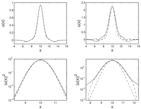
Figure 1: Comparison of the lattice reconstructed solution in the tight-binding (dashed line) and the 3-band (dash-dotted line) approximation with the exact solution (solid line). The comparison is performed for $V(x)=-5\cos(2x)$ and different chemical potentials: $\mu=1.5$ (left panels) and $\mu=-1.5$ (right panels). The bottom (semi-log) panels show the result of dynamical time-evolution of the tight-binding approximation with the dotted line. As time evolves (we depict snapshots at $t\approx 50$), the latter can be seen to approach the shape of the exact solution (in the left panel, these plots cannot be distinguished) and to match its asymptotic form, possibly shedding small wakes of low-amplitude wave radiation in the process (see, for example, the bottom right panel).

At this stage, one can study the ILMs of Eqs. (27) or (28) and use the Wannier function expansion to reconstruct the solution of the original GP equation Alfimov et al. (2002a). This approach has been successfully used in a variety of applications and for different localized states present in the lattice—including bright, dark, and discrete-gap solitons, as well as breathers Abdullaev et al. (2001); Trombettoni and Smerzi (2001); Kevrekidis et al. (2003d); Alfimov et al. (2002b). Other phenomena, such as discrete modulational instabilities, have also been studied Kevrekidis and Frantzeskakis (2004). More specifically, one of the most successful implementations of discrete NLS equations (and variants thereof) in this context included the quantitative prediction that its modulational stability analysis determined the threshold of a dynamical instability of the condensate (the so-called classical superfluid-insulator transition of Smerzi et al. (2002)). These predictions were subsequently verified quantitatively by the experimental measurements of Ref. Cataliotti et al. (2003).

IV Soliton-soliton tail-mediated interactions and the Toda lattice

Recent advances in trapping techniques allow the generation of bright solitons and chains of bright solitons in effectively 1D attractive condensates Strecker et al. (2002); Khawaja et al. (2002); Strecker et al. (2003); Khaykovich et al. (2002). In this section, we consider the collective motion of a chain of bright solitons. We focus, in particular, on the dynamics of attractive BECs trapped in a deep optical lattice (OL) that renders a 1D attractive condensate into a chain of interacting solitons (see Fig. 2).

Consider a BEC loaded into an OL potential produced by the interference pattern of multiple counter-propagating laser beams Anderson and Kasevich (1998a); Jona-Lasinio et al. (2003); Konotop et al. ; Orzel et al. (2001a); Morsch et al. (2001a); Cataliotti et al. (2001); Greiner et al. (2001); Greiner et al. (2002a). In principle, it is possible to design various optical trap profiles (essentially at will) by appropriately superimposing interference patterns. For the purposes of this exposition, we adopt an OL profile, with a tunable inter-well separation, given by the Jacobi elliptic-sine function,

$$V(x)=V_{0}\,\mathrm{sn}^{2}(x;k)\,,$$ (29)

where $V_{0}$ is the strength of the OL. The elliptic modulus $k$ allows one to tune the separation between consecutive wells, $r\equiv\xi_{0;j+1}-\xi_{0;j}=2K(k)$, where $\xi_{0;j}=2j\,K(k)$ is the position of the $j$-th well and $K(k)$ is the complete elliptic integral of the first kind.

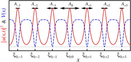
Figure 2: A quasi-1D condensate (solid line) in a deep periodic optical-lattice potential (dashed line). The condensate is effectively described as a chain of coupled solitons whose positions follow a Toda lattice with on-site potentials [Eq. (33)]. Using the oscillating ansatz (34), where the $j$-th soliton is forced to oscillate with amplitude $A_{j}$, one can further reduce the dynamics to a second-order recurrence relationship between neighboring amplitudes [Eq. (35)].

The stability properties of BECs in the optical lattice potential (29) have been recently studied Bronski et al. (2001a, c, b). Here, we are interested in the case of large separation between the wells ($k\simeq 1$), when the BEC is effectively fragmented into a chain of nearly identical solitons with tail-mediated interactions, subject to the action of an effective on-site potential due to the OL. For a large set of parameter values, the system can be reduced to a Toda lattice Toda (1989), as was illustrated in Refs. Carretero-González and Promislow (2002); Carretero-González and Promislow (2004). The reduction involves two steps.

First, the interaction between the $j$-th soliton [at position $\xi_{j}(t)$] and the $j$-th well is approximated, using variational techniques Malomed (2002) or methods based on conserved quantities Carretero-González and Promislow (2004), by

$$\ddot{\xi}_{j}=-V_{\mathrm{eff}}^{\prime}(\xi_{j}-\xi_{0;j})\,,$$ (30)

which describes a particle in the effective potential $V_{\mathrm{eff}}$ felt by the soliton. For well-separated troughs ($k\simeq 1$), the effective potential may be approximated by Carretero-González and Promislow (2004)

$$V_{\mathrm{eff}}^{\prime}(\xi)\approx\nu V_{0}\left(a_{1}\xi-\frac{224}{1125}\xi V_{0}+a_{3}\xi^{3}\right)\,,$$ (31)

where $\nu$ is the average amplitude (height) of the soliton, $a_{1}=8/15$ and $a_{3}=-16/63$.

Second, one treats the interaction of consecutive solitons in the absence of the OL. This interaction is well-studied in the context of optical solitons Karpman and Solov’ev (1981a, b); Gerdjikov et al. (1996, 1997); Arnold (1998, 1999); Malomed (2002). For identical, well-separated solitons (with the phase difference $\pi$ between adjacent solitons), it is approximated by the Toda-lattice equation for the soliton positions,

$$\begin{array}[]{rcl}\ddot{\xi}_{j}&=&T_{L}(\xi_{j-1},\xi_{j},\xi_{j+1})\\[8.61108pt] &=&8\nu^{3}\,\left(e^{-\nu(\xi_{j}-\xi_{j-1})}-e^{-\nu(\xi_{j+1}-\xi_{j})}\right)\,.\end{array}$$ (32)

Finally, after combining (32) with the on-site potential dynamics (30), we reduce the dynamics of a weakly coupled BEC in the deep OL to the Toda lattice with on-site potentials,

$$\ddot{\xi}_{j}=T_{L}(\xi_{j-1},\xi_{j}\,,\xi_{j+1})-V_{\mathrm{eff}}^{\prime}(\xi_{j}-\xi_{0;j})\,.$$ (33)

The Toda lattice (32) admits exact traveling-soliton solutions Toda (1989). However, the effective potential in (33) breaks the lattice’s translational invariance and accommodates the existence of ILMs (breathers). To describe such localized oscillations, we consider small vibrations about the equilibrium state ($\xi_{j}=\xi_{0;j}$):

$$\xi_{j}(t)=\xi_{0;j}+A_{j}\,\cos(\omega t)\,,$$ (34)

where $\omega$ is the common oscillation frequency for all solitons, and the $j$-th soliton vibrates with an amplitude $A_{j}$ about its equilibrium position $\xi_{0;j}$ (see Fig. 2). Substituting the ansatz (34) into Eq. (33) and discarding higher-order modes yields a recurrence relationship between consecutive amplitudes,

$$A_{n+1}=(a+b\,A_{n}^{2})\,A_{n}-A_{n-1}\,,$$ (35)

where $a=2-\omega^{2}+4a_{1}d$, $b=3a_{3}d$, $d=e^{\nu r}/(16\nu^{4})$, $r$ is the separation between adjacent troughs, and $a_{1}$ and $a_{3}$ are the coefficients from the expansion of the effective potential (31). Note that the method just described is applicable to any OL profile that reduces the dynamics of a single soliton to that of a particle inside an effective potential given by a cubic polynomial in $\xi$.

By defining consecutive oscillation amplitudes as $y_{n}\equiv A_{n}$ and $x_{n}\equiv A_{n-1}$, the recurrence relationship (35) can be cast as a 2D map,

$$\left\{\begin{array}[]{rcl}x_{n+1}&=&y_{n}\\[8.61108pt] y_{n+1}&=&(a+b\,y_{n}^{2})\,y_{n}-x_{n}\end{array}\right.\,.$$ (36)

It is crucial to note here that the iteration index $n$ in (36) corresponds to the spatial lattice-site index for the soliton chain. Thus, forward (backward) iteration of the 2D map (36) amounts to a right (left) shift of the spatial position in the soliton chain. As our goal is to find spatially localized states of the BEC chain (i.e., ILMs), we are interested in finding solutions of Eq. (35) for which $A_{n}\rightarrow 0$ as $n\rightarrow\pm\infty$ and $A_{0}>0$ (see Fig. 2). That is, $(x_{n},y_{n})\rightarrow(0,0)$ as $n\rightarrow\pm\infty$. These solutions correspond to homoclinic connections of the origin.

A typical intersection for the stable (solid curve) and unstable (dashed curve) manifolds of the 2D map (36) is depicted in the top-left panel of Fig. 3. The intersection points $P_{i}$ between the stable and unstable manifolds then generate a localized configuration for the recurrence relationship (35), as depicted in the top-right panel of Fig. 3. When this localized configuration is inserted into the original GP equation (14), one obtains a spatially localized, multi-soliton state (depicted in the bottom panel of Fig. 3) by shifting each soliton from its equilibrium position by the prescribed amount Carretero-González and Promislow (2002); Carretero-González and Promislow (2004).

  

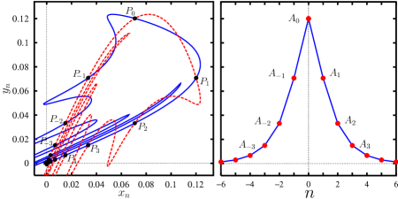
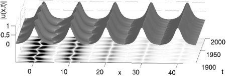
Figure 3: Homoclinic connection of the origin (top-left panel) [from Ref. Carretero-González and Promislow (2002)], giving rise to a spatially localized profile (top-right panel). Bottom: the localized state in the original BEC model (14) generated by the prescribed amplitude configuration. The shaded base, depicting $\partial|u|/\partial t$, highlights the areas in which the atomic density $|u(x,t)|$ varies the most. Observe that the solution decays as one moves away from the center ($x=0$). (As the solution is symmetric with respect to $x=0$, only its right-hand side is shown.)

It is important to note that generic localized initial configurations do not give rise to long-lived, self-sustained ILMs. Nonetheless, the construction described above is quite efficient in producing approximate initial configurations that generate clean and robust localized states, such as the one displayed in Fig. 3. The structural and dynamical stability of these localized states is quite interesting. For example, the structural stability of the homoclinic tangle of the 2D map guarantees the existence of the ILM solution in the original model (14), despite the employment of various approximations in the former’s derivation. On the other hand, the dynamical stability of ILMs permits their observation even in the presence of strong perturbations (such as noise). Indeed, numerical experiments show that ILMs prevail even in the presence of large perturbations to the initial configuration or strong numerical noise, as discussed in Refs. Carretero-González and Promislow (2002); Carretero-González and Promislow (2004).

Finally, it is worth mentioning that the dynamical reduction to the 2D map (36) can also be used to generate—in addition to the localized states discussed above—a wide range of spatiotemporal structures by following the map’s fixed points, periodic orbits, quasi-periodic orbits, and even chaotic orbits. Further, the techniques described in this section can also be applied to chains of bright solitons in which the deep OL is replaced by an array of focused laser beams or impurities that tends to pin the solitons and serve as a local effective attractive potential [see Eq. (30)].

V Conclusions

In this work, we have surveyed recent research on lattice dynamics of Bose-Einstein condensates (BECs) in optical lattice (OL) potentials. We discussed, in particular, the dynamics of BECs in a deep OL that naturally discretizes the original spatially continuous system into a collection of discrete interacting nodes (wells). The ensuing nonlinear lattice features the trademark localized solutions—solitons and intrinsic localized modes—that have rendered the Fermi-Pasta-Ulam problem one of last century’s most important contributions to nonlinear science. Specifically, using Wannier-function expansions, we reduced the dynamics of the Gross-Pitaevskii (GP) equation to a discrete nonlinear Schrödinger (DNLS) equation, which was subsequently used to identify localized solutions (as well as a number of other interesting dynamical instabilities, such as those discussed in Ref. Kevrekidis and Frantzeskakis (2004)) and reconstruct the nonlinear waves of the original GP equation. Treating a BEC trapped in a strong OL as a collection of interacting solitons, we then used perturbative and/or variational techniques to reduce the original GP equation to a Toda-lattice equation with an effective on-site potential. This nonlinear lattice supports robust, exponentially localized oscillations in BEC soliton chains.

The crucial ingredient, amenable to the dynamical systems perspective described in this manuscript, is the GP equation’s nonlinear self-interaction, which is induced as a mean-field representation of two-particle interactions and is responsible for a plethora of dynamical behaviors. The most remarkable of these, solitary waves (solitons), lie at the heart of the paradigm that originated from the seminal work of Fermi, Pasta, and Ulam.

There remain, moreover, a multitude of exciting directions for future research. For example, the study of nonlinear lattice models in higher dimensions has yielded a number of interesting generalizations and more exotic solitary waves such as multi-dimensional solitons Kevrekidis et al. (2001) and discrete vortices Malomed and Kevrekidis (2001); Kevrekidis et al. (2004). A systematic analysis of their existence properties, dynamical characteristics (mobility and structural stability), thermodynamic properties, and physical relevance involves a number of interesting and subtle questions that may keep nonlinear scientists like us busy until we’re ready to celebrate the 100th anniversary of the publication of the FPU problem.

References

- Weissert (1997) T. P. Weissert, The Genesis of Simulation in Dynamics: Pursuing the Fermi-Pasta-Ulam Problem (Springer-Verlag, New York, NY, 1997).
- Davis et al. (1995) K. B. Davis, M.-O. Mewes, M. R. Andrews, N. J. van Druten, D. S. Durfee, D. M. Kurn, and W. Ketterle, Phys. Rev. Lett. 75, 3969 (1995).
- Anderson et al. (1995) M. H. Anderson, J. R. Ensher, M. R. Matthews, C. E. Wieman, and E. A. Cornell, Science 269, 198 (1995).
- Zabusky (1984) N. J. Zabusky, Physics Today pp. 2–12 (1984).
- Friesecke and Pego (1999) G. Friesecke and R. L. Pego, Nonlinearity 12, 1601 (1999).
- Friesecke and Pego (2002) G. Friesecke and R. L. Pego, Nonlinearity 15, 1343 (2002).
- Friesecke and Pego (2004a) G. Friesecke and R. L. Pego, Nonlinearity 17, 207 (2004a).
- Friesecke and Pego (2004b) G. Friesecke and R. L. Pego, Nonlinearity 17, 229 (2004b).
- Lepri et al. (2003) S. Lepri, R. Livi, and A. Politi, Physics Reports 377, 1 (2003).
- Fermi et al. (1955) E. Fermi, J. R. Pasta, and S. Ulam, Tech. Rep. Report LA-1940, Los Alamos (1955).
- Lichtenberg and Lieberman (1992) A. J. Lichtenberg and M. A. Lieberman, Regular and Chaotic Dynamics, no. 38 in Applied Mathematical Sciences (Springer-Verlag, New York, NY, 1992), 2nd ed.
- Ablowitz and Clarkson (1991) M. J. Ablowitz and P. A. Clarkson, Solitons, Nonlinear Evolution Equations and Inverse Scattering, no. 149 in London Mathematical Society Lecture Notes Series (Cambridge University Press, Cambridge, U.K., 1991).
- Zabusky and Kruskal (1965) N. J. Zabusky and M. D. Kruskal, Phys. Rev. Lett. 15, 240 (1965).
- Dodd et al. (1982) R. Dodd, J. Eilbeck, J. Gibbon, and H. Morris, Solitons and Nonlinear Wave Equations (London: Academic Press, London, UK, 1982).
- Drazin and Johnson (1989) P. Drazin and R. Johnson, Solitons: An Introduction (Cambridge University Press, Cambridge, UK, 1989).
- Whitham (1974) G. B. Whitham, Linear and Nonlinear Waves, Pure and Applied Mathematics (Wiley-Interscience, New York, NY, 1974).
- Ablowitz and Segur (1981) M. J. Ablowitz and H. Segur, Solitons and the Inverse Scattering Transform, SIAM Studies in Applied Mathematics (Society for Industrial and Applied Mathematics, Philadelphia, Pennsylvania, 1981).
- Pethick and Smith (2002) C. J. Pethick and H. Smith, Bose-Einstein Condensation in Dilute Gases (Cambridge University Press, Cambridge, United Kingdom, 2002).
- Dalfovo et al. (1999) F. Dalfovo, S. Giorgini, L. P. Pitaevskii, and S. Stringari, Rev. Mod. Phys. 71, 463 (1999).
- Alfimov et al. (2002a) G. L. Alfimov, P. G. Kevrekidis, V. V. Konotop, and M. Salerno, Phys. Rev. E 66 (2002a).
- Izrailev and Chirikov (1966) F. M. Izrailev and B. V. Chirikov, Soviet Physics Doklady 11, 30 (1966).
- Driscoll and O’Neil (1976) C. F. Driscoll and T. M. O’Neil, Phys. Rev. Lett. 37, 69 (1976).
- Kruskal (1975) M. Kruskal, in Dynamical Systems Theory and Applications, edited by J. Moser (Springer-Verlag, New York, NY, 1975), vol. 38 of Lecture Notes in Physics, pp. 310–354, Seattle 1974.
- Newell (1974) A. C. Newell, ed., Nonlinear Wave Motion, vol. 15 of Lectures in Applied Mathematics (American Mathematical Society, Providence, Rhode Island, 1974).
- Rink (2002) B. Rink, J. Nonlin. Sci. 12, 479 (2002).
- Rink (2003) B. Rink, Physica D 175, 31 (2003).
- Rink (2001) B. Rink, Comm. Math. Phys. 218, 665 (2001).
- Biello et al. (2002) P. R. Kramer, J. A. Biello, and Y. Lvov, in Proceedings of the 4th International Conference on Dynamical Systems and Differential Equations (2002), nlin.CD/0210007.
- Gerdjikov et al. (1996) V. S. Gerdjikov, D. J. Kaup, I. M. Uzunov, and E. G. Evstatiev, Phys. Rev. Lett. 77, 3943 (1996).
- Berman and Kolovskii (1984) G. P. Berman and A. R. Kolovskii, Soviet Physics JETP 60, 1116 (1984).
- Ketterle (1999) W. Ketterle, Physics Today 52, 30 (1999).
- Burnett et al. (1999) K. Burnett, M. Edwards, and C. W. Clark, Physics Today 52, 37 (1999).
- Köhler (2002) T. Köhler, Phys. Rev. Lett. 89, 210404 (2002).
- Baizakov et al. (2002) B. B. Baizakov, V. V. Konotop, and M. Salerno, J. Phys. B: Atom. Mol. Phys. 35, 5105 (2002).
- Salasnich et al. (2002a) L. Salasnich, A. Parola, and L. Reatto, J. Phys. B: Atom. Mol. Phys. 35, 3205 (2002a).
- Pérez-García et al. (1998) V. Pérez-García, H. Michinel, and H. Herrero, Phys. Rev. A 57, 3837 (1998).
- Salasnich et al. (2002b) L. Salasnich, A. Parola, and L. Reatto, Phys. Rev. A 66, 043603 (2002b).
- Band et al. (2003) Y. B. Band, I. Towers, and B. A. Malomed, Phys. Rev. A 67, 023602 (2003).
- Lieb et al. (2003) E. H. Lieb, R. Seiringer, and J. Yngvason, Phys. Rev. Lett. 91, 150401 (2003).
- Gross (1961) E. P. Gross, Nuovo Cim. 20, 454 (1961).
- Pitaevskii (1961) L. P. Pitaevskii, Sov. Phys. JETP 13, 451 (1961).
- Donley et al. (2001) E. A. Donley, N. R. Claussen, S. L. Cornish, J. L. Roberts, E. A. Cornell, and C. E. Weiman, Nature 412, 295 (2001).
- Kevrekidis et al. (2003a) P. G. Kevrekidis, G. Theocharis, D. J. Frantzeskakis, and B. A. Malomed, Phys. Rev. Lett. 90, 230401 (2003a).
- Anderson and Kasevich (1998a) B. P. Anderson and M. A. Kasevich, Science 282, 1686 (1998a).
- Jona-Lasinio et al. (2003) M. Jona-Lasinio, O. Morsch, M. Cristiani, N. Malossi, J. H. Müller, E. Courtade, M. Anderlini, and E. Arimondo, Phys. Rev. Lett. 91, 230406 (2003).
- (46) V. V. Konotop, P. G. Kevrekidis, and M. Salerno, cond-mat/0404608.
- Orzel et al. (2001a) C. Orzel, A. K. Tuchman, M. L. Fenselau, M. Yasuda, and M. A. Kasevich, Science 291, 2386 (2001a).
- Morsch et al. (2001a) O. Morsch, J. H. Müller, M. Cristiani, D. Ciampini, and E. Arimondo, Phys. Rev. Lett. 87, 140402 (2001a).
- Cataliotti et al. (2001) F. S. Cataliotti, S. Burger, C. Fort, P. Maddaloni, F. Minardi, A. Trombettoni, A. Smerzi, and M. Inguscio, Science 293, 843 (2001).
- Greiner et al. (2001) M. Greiner, I. Bloch, O. Mandel, T. W. Hänsch, and T. Esslinger, Phys. Rev. Lett. 87, 160405 (2001).
- Greiner et al. (2002a) M. Greiner, O. Mandel, T. Esslinger, T. W. Hänsch, and I. Bloch, Nature 415, 39 (2002a).
- Anderson and Kasevich (1998b) B. P. Anderson and M. A. Kasevich, Science 282, 1686 (1998b).
- Greiner et al. (2002b) M. Greiner, O. Mandel, T. Esslinger, T. Hänsch, and I. Bloch, Nature 415 (2002b).
- Burger et al. (2001) S. Burger, F. S. Cataliotti, C. Fort, F. Minardi, and M. Inguscio, Phys. Rev. Lett. 86, 4447 (2001).
- Morsch et al. (2001b) O. Morsch, J. H. Müller, M. Christiani, D. Ciampini, and E. Arimondo, Phys. Rev. Lett. 87 (2001b).
- Choi and Niu (1999) D.-I. Choi and Q. Niu, Phys. Rev. Lett. 82, 2022 (1999).
- Jaksch et al. (1998) D. Jaksch, C. Bruder, J. I. Cirac, C. W. Gardiner, and P. Zoller, Phys. Rev. Lett. 81, 3108 (1998).
- Peil et al. (2003) S. Peil, J. V. Porto, B. Laburthe Tolra, J. M. Obrecht, B. E. King, M. Subbotin, S. L. Rolston, and W. D. Phillips, Phys. Rev. A 67 (2003).
- Rey et al. (2003) A. M. Rey, B. L. Hu, E. Calzetta, A. Roura, and C. Clark, Phys. Rev. A 69, 033610 (2004).
- Porter and Cvitanović (2004a) M. A. Porter and P. Cvitanović, Phys. Rev. E 69 (2004a), arXiv: nlin.CD/0307032.
- Porter and Kevrekidis (2004) M. A. Porter and P. G. Kevrekidis (2004), arXiv: nlin.PS/0406063.
- Bronski et al. (2001a) J. C. Bronski, L. D. Carr, B. Deconinck, and J. N. Kutz, Phys. Rev. Lett. 86, 1402 (2001a).
- Kevrekidis et al. (2003b) P. Kevrekidis, R. Carretero-González, G. Theocharis, D. Frantzeskakis, and B. Malomed, J. Phys. B 36, 3467 (2003b).
- Kevrekidis et al. (2003c) P. Kevrekidis, D. Frantzeskakis, B. Malomed, A. Bishop, and I. Kevrekidis, New J. Phys. 5, 64.1 (2003c).
- Kevrekidis et al. (2003d) P. Kevrekidis, R. Carretero-González, G. Theocharis, D. Frantzeskakis, and B. Malomed, Phys. Rev. A 68, 035602 (2003d).
- Orzel et al. (2001b) C. Orzel, A. K. Tuchman, M. L. Fenselau, M. Yasuda, and M. A. Kasevich, Science 291, 2386 (2001b).
- Smerzi et al. (2002) A. Smerzi, A. Trombettoni, P. G. Kevrekidis, and A. R. Bishop, Phys. Rev. Lett. 89, 170402 (2002).
- Cataliotti et al. (2003) F. S. Cataliotti, L. Fallani, F. Ferlaino, C. Fort, P. Maddaloni, and M. Inguscio, New J. Phys. 5, 71.1 (2003).
- Porto et al. (2003) J. V. Porto, S. Rolston, B. Laburthe Tolra, C. J. Williams, and W. D. Phillips, Philosophical Transactions: Mathematical, Physical & Engineering Sciences 361, 1417 (2003).
- Vollbrecht et al. (2004) K. G. H. Vollbrecht, E. Solano, and J. L. Cirac (2004), arXiv: quant-ph/0405014.
- Porter and Cvitanović (2004b) M. A. Porter and P. Cvitanović, Chaos 14, 739 (2004b),
- Bronski et al. (2001b) J. C. Bronski, L. D. Carr, R. Carretero-González, B. Deconinck, J. N. Kutz, and K. Promislow, Phys. Rev. E 64 (2001b).
- Bronski et al. (2001c) J. C. Bronski, L. D. Carr, B. Deconinck, J. N. Kutz, and K. Promislow, Phys. Rev. E 63 (2001c).
- Alfimov et al. (2002b) G. L. Alfimov, V. V. Konotop, and M. Salerno, Europhys. Lett. 58, 7 (2002b).
- Louis et al. (2003) P. J. Y. Louis, E. A. Ostrovskaya, C. M. Savage, and Y. S. Kivshar, Phys. Rev. A 67 (2003).
- Konotop and Salerno (2002) V. V. Konotop and M. Salerno, Phys. Rev. A 65 (2002).
- Sakaguchi and Malomed (2004) H. Sakaguchi and B. Malomed, J. Phys. B 37, 1443 (2004).
- Abdullaev et al. (2001) F. Abdullaev, B. B. Baizakov, S. A. Darmanyan, V. V. Konotop, and M. Salerno, Phys. Rev. A 64 (2001).
- Kevrekidis and Frantzeskakis (2004) P. G. Kevrekidis and D. J. Frantzeskakis, Modern Phys. Lett. B 18, 173 (2004).
- Ashcroft and Mermin (1976) N. W. Ashcroft and N. D. Mermin, Solid State Physics (Brooks/Cole, Australia, 1976).
- Trombettoni and Smerzi (2001) A. Trombettoni and A. Smerzi, Phys. Rev. Lett. 86, 2353 (2001).
- Strecker et al. (2002) K. E. Strecker, G. B. Partridge, A. G. Truscott, and R. G. Hulet, Nature 417, 150 (2002).
- Khawaja et al. (2002) U. A. Khawaja, H. T. C. Stoof, R. G. Hulet, K. E. Strecker, and G. B. Partridge, Phys. Rev. Lett. 89, 200404 (2002).
- Strecker et al. (2003) K. E. Strecker, G. B. Partridge, A. G. Truscott, and R. G. Hulet, New J. Phys. 5, 73.1 (2003).
- Khaykovich et al. (2002) L. Khaykovich, F. Schreck, G. Ferrari, T. Bourdel, J. Cubizolles, L. D. Carr, Y. Castin, and C. Salomon, Science 296, 1290 (2002).
- Toda (1989) M. Toda, Theory of Nonlinear Lattices. (Springer-Verlag, 1989), 2nd ed.
- Carretero-González and Promislow (2002) R. Carretero-González and K. Promislow, Phys. Rev. A 66 (2002).
- Carretero-González and Promislow (2004) R. Carretero-González and K. Promislow (2004), in preparation.
- Malomed (2002) B. Malomed, Progress in Optics 43, 69 (2002).
- Karpman and Solov’ev (1981a) V. I. Karpman and V. V. Solov’ev, Physica D 3, 142 (1981a).
- Karpman and Solov’ev (1981b) V. I. Karpman and V. V. Solov’ev, Physica D 3, 487 (1981b).
- Gerdjikov et al. (1997) V. S. Gerdjikov, I. M. Uzunov, E. G. Estaviev, and G. L. Diankov, Phys. Rev. E 55, 6039 (1997).
- Arnold (1998) J. M. Arnold, J. Opt. Soc. Am. A 15, 1450 (1998).
- Arnold (1999) J. M. Arnold, Phys. Rev. E 60, 979 (1999).
- Kevrekidis et al. (2001) P. Kevrekidis, K. Rasmussen, and A. Bishop, Int. J. Mod. Phys. B 15, 2833 (2001).
- Malomed and Kevrekidis (2001) B. Malomed and P. Kevrekidis, Phys. Rev. E 64, 026601 (2001).
- Kevrekidis et al. (2004) P. Kevrekidis, B. Malomed, D. Frantzeskakis, and R. Carretero-González, Phys. Rev. Lett. 93, 080403 (2004).