Lyapunov modes in soft-disk fluids

Abstract

Lyapunov modes are periodic spatial perturbations of phase-space states of many-particle systems, which are associated with the small positive or negative Lyapunov exponents. Although familiar for hard-particle systems in one, two, and three dimensions, they have been difficult to find for soft-particles. We present computer simulations for soft-disk systems in two dimensions and demonstrate the existence of the modes, where also Fourier-transformation methods are employed. We discuss some of their properties in comparison with equivalent hard-disk results. The whole range of densities corresponding to fluids is considered. We show that it is not possible to represent the modes by a two-dimensional vector field of the position perturbations alone (as is the case for hard disks), but that the momentum perturbations are simultaneously required for their characterization.

I Introduction

For the last 50 years molecular dynamics simulations have decisively contributed to our understanding of the structure and dynamics of simple fluids and solids Alder:1959 . More recently, also the concepts of dynamical systems theory have been applied to study the tangent-space dynamics of such systems posch:1988a . Of particular interest is the extreme sensitivity of the phase-space evolution to small perturbations. On average, such perturbations grow, or shrink, exponentially with time, which may be characterized by a set of rate constants, the Lyapunov exponents. The whole set of exponents is referred to as the Lyapunov spectrum. This instability is at the heart of the ergodic and mixing properties of a fluid and offers a new tool for the study of the microscopic dynamics. In particular, it was recognized very early that there is a close connection with the classical transport properties of systems in nonequilibrium stationary states hhp87 . For fluids in thermodynamic equilibrium, an analysis of the Lyapunov instability is expected to provide an unbiased expansion of the dynamics into events, which, in favorable cases, may be associated with qualitatively different degrees of freedom, such as the translation and rotation of linear molecules mph98 , or with the intra-molecular rotation around specific chemical bonds p05 .

Since the pioneering work of Bernal Bernal:1968 with steel balls, hard disks have been considered the simplest model for a “real” fluid. With respect to the structure, they serve as a reference system for highly-successful perturbation theories of liquids Hansen:1991 ; Reed:1973 . Recently we studied the Lyapunov instability of such a model and found mathII ; pf04 ; hpfdz02 ; Milanovic:2002 ; EFPZ04

1. that the slowly-growing and decaying perturbations associated with the non-vanishing Lyapunov exponents closest to zero may be represented as periodic vector fields coherently spread out over the physical space and with well-defined wave vectors $k$. Because of their similarity with the classical modes of fluctuating hydrodynamics we refer to them as Lyapunov modes. Depending on the boundary conditions, the respective exponents are degenerate, and the spectrum has a step-like appearance in that regime.

2. that the fast-growing or decaying perturbations are localized in space, and the number of particles actively contributing at any instant of time vanishes in the thermodynamic limit.

Experimentally, the Lyapunov modes were found for hard-particle systems in one, two and three dimensions and for various boundary conditions, provided that the system size, $L$, in at least one direction is large enough for the discrete particles to generate a recognizable wave-like pattern with a wave number $k$. Their theoretical understanding is based on the spontaneous breaking of the translational symmetry of the zero modes $(k=0)$, which are associated with the vanishing Lyapunov exponents and are a consequence of the conservation laws in the system eg00 ; MM01 ; MM04 ; WB04 ; EFPZ04 ; Morriss:2004 .

Based on this experimental and theoretical evidence for hard-particle systems, it is natural to expect that the Lyapunov modes are a general feature of many-body systems with short-range interactions and that the details of the pair potential should not matter. However, already our very first simulations with soft disks in two dimensions hpfdz02 ; Dellago:2002 ; pf04 revealed a much more complicated scenario. Whereas the spatial localization of the fast-growing or decaying perturbations could be easily verified, the mode structure for the slowly-growing or decaying perturbations was elusive and could, at first, not be unambiguously detected. Here we demonstrate that the modes for soft sphere fluids do indeed exist. However, sophisticated Fourier-transformation techniques are needed to prove their existence. Interestingly, the degeneracy of the Lyapunov exponents and, hence, the step structure of the spectrum so familiar from the hard-disk case is recovered, but only for low densities. This suggests that kinetic theory is a proper theoretical framework in that case. For intermediate and large-density soft-disk fluids the degeneracy disappears. We do not have an explanation for this fact. Most recently, Lyapunov modes were demonstrated by Radons and Yang ry04a ; ry04b for one-dimensional Lennard-Jones fluids at low temperatures and densities.

In this work we analyze the Lyapunov instability of repulsive Weeks-Chandler-Anderson (WCA) disks in two dimensions and compare it to analogous hard-disk results. The main difficulty is the large box size required for the modes to develop and, hence, the large number of particles, $N$. It requires parallel programming for the computation of the dynamics both in phase and tangent space and for the re-normalization of the perturbation vectors according to the classical algorithms of Benettin et al. Benettin and Shimada et al. Shimada . In Sec. II we characterize the systems and summarize the numerical methods used. In Sec. III we discuss the surprising differences found between the Lyapunov spectra for the soft- and hard-particle fluids, particularly at intermediate and large densities. Sec.IV is devoted to an analysis of the zero modes associated with the vanishing Lyapunov exponents. The Lyapunov modes are analyzed in Secs. V and VI. We close with some concluding remarks in Sec. VII.

II Characterization of the system and methodology

We consider $N$ disks with equal mass $m$ in a two-dimensional rectangular box with extensions $L_{x}$ and $L_{y}$ and aspect ration $A\equiv L_{y}/L_{x}$. Periodic boundary conditions are used throughout. The particles interact with a smooth repulsive potential, for which we consider two cases:
i) a Weeks-Chandler-Anderson potential,

$$\phi_{WCA}=\left\{\begin{array}[]{ll}4\epsilon\left[\left(\frac{\sigma}{r}\right)^{12}-\left(\frac{\sigma}{r}\right)^{6}\right]+\epsilon,&\qquad r\leq 2^{1/6}\sigma\\ 0,&\qquad r>2^{1/6}\sigma\end{array}\right.,$$ (1)

with a force cutoff at $r=2^{1/6}\sigma$. As usual, $\sigma$ and $\epsilon$ are interaction-range and energy parameters, respectively, which are ultimately set to unity. Actually, such a potential is not the best choice, since the forces and their derivatives (required for the dynamics in tangent-space) are not continuous at the cutoff. This introduces additional noise into the simulation and violates the conservation laws. It also affects the computation of the Lyapunov spectrum. To avoid this problem we sometimes also use
ii) a power-law potential,

$$\phi_{PL}=\left\{\begin{array}[]{ll}100\epsilon\left[1-\left(\frac{r}{\sigma}\right)^{2}\right]^{4},&\qquad r\leq\sigma\\ 0,&\qquad r>\sigma\end{array}\right.$$ (2)

which looks very similar but does not suffer from this deficiency. We mention, however, that the results discussed below turn out to be insensitive to this weakness of the WCA potential. For reasons of comparison we also consider
iii) a hard-disk potential,

$$\phi_{HD}=\left\{\begin{array}[]{ll}\infty,&\qquad r\leq\sigma\\ 0,&\qquad r>\sigma\end{array}\right.$$ (3)

The phase space, $X$, has $4N$ dimensions, and a phase point $\Gamma\in X$ is given by the $4N$-dimensional vector $\Gamma(t)=\{q_{i},p_{i};i=1,\dots,N\}$, where $q_{i}$ and $p_{i}$, denote the respective positions and momenta of the disks. It evolves according to the time-reversible motion equations

$$\dot{\Gamma}=F(\Gamma),$$ (4)

which are conveniently written as a system of first order differential equations. Here, $F(\Gamma)=\{\frac{p_{i}}{m},-\frac{\partial\Phi}{\partial q_{i}};i=1,\dots,N\}$ follows from Hamilton’s equations, where $\Phi\equiv\sum_{i}\sum_{j>i}\phi(|q_{i}-q_{j}|)$ is the total potential energy.

Any infinitesimal perturbation $\delta\Gamma_{l}=\{\delta q_{i}^{(l)},\delta p_{i}^{(l)};i=1,\dots,N\}$ lies in the tangent space $TX$, tangent to the manifold $X$ at the phase point $\Gamma(t)$. Here, $\delta q_{i}^{(l)},$ and $\delta p_{i}^{(l)}$ are two-dimensional vectors and denote the position and momentum perturbations contributed by particle $i$. $\delta\Gamma_{l}$ evolves according to the linearized equations of motion

$$\dot{\delta\Gamma_{l}}=\frac{\partial F}{\partial\Gamma_{l}}\cdot\delta\Gamma_{l}.$$ (5)

Oseledec’s theorem Oseledec:1968 assures us that there exist $4N$ orthonormal initial tangent vectors $\delta\Gamma_{l}(0),l=1,\dots,4N$, whose norm grows or shrinks exponentially with time such that the Lyapunov exponents

$$\lambda_{l}=\lim_{t\to\infty}\frac{1}{t}\ln\frac{||\delta\Gamma_{l}(t)||}{||\delta\Gamma_{l}(0)||},\quad l=1,\dots,4N,$$ (6)

exist. However, in the course of time these vectors would all get exponentially close to the most-unstable direction and diverge, since the unconstrained flow in tangent space does not preserve the orthogonality of these vectors. In the classical algorithms of Benettin et al. Benettin , and Shimada et al. Shimada also used in this work, this difficulty is circumvented by replacing these vectors by a set of modified tangent vectors, ${\delta_{l},l=1,\dots,4N}$, which are periodically re-orthonormalized with a Gram-Schmidt procedure. The Lyapunov exponents are determined from the time-averaged renormalization factors. The vectors $\delta_{l}$ represent the perturbations associated with $\lambda_{l}$ and are the objects analyzed below. Henceforth we use the notation $\delta q_{i}^{(l)},$ and $\delta p_{i}^{(l)}$ also for the individual particle contributions to the ortho-normalized vectors, $\delta_{l}=\{\delta q_{i}^{(l)},\delta p_{i}^{(l)};i=1,\dots,N\}$. For later use, we introduce also the squared norm in the single-particle $\mu$ space,

$$\gamma_{i}^{(l)}\equiv\left(\delta q_{i}^{(l)}\right)^{2}+\left(\delta p_{i}^{(l)}\right)^{2}.$$ (7)

This quantity is bounded, $0\leq\gamma_{i}^{(l)}\leq 1$, and obeys the sum rule $\sum_{i=1}^{N}\gamma_{i}^{(l)}=1$ for any $l$. Since the equations (5) are linear in $\delta\Gamma_{l}$, the quantities $\gamma_{i}^{(l)}$ indicate, how the activity for perturbation growth, as measured by $\lambda_{l}$, is distributed over the particles at any instant of time.

For the hard-disk systems the motion equations (4) and (5) need to be generalized to include also the collision maps due to the instantaneous particle collisions. For algorithmic details we refer to our previous work dph96 ; dp97 ; mathII .

The exponents are taken to be ordered by size, $\lambda_{l}\geq\lambda_{l+1}$, where the index $l$ numbers the exponents. According to the conjugate pairing rule for symplectic systems Evans:1990 ; Ruelle:1999 , the exponents appear in pairs such that the respective pair sums vanish, $\lambda_{l}+\lambda_{4N+1-l}=0$. Only the positive half of the spectrum needs to be calculated. Furthermore, six of the exponents, $\{\lambda_{2N-2\leq l\leq 2N+3}\}$, vanish as a consequence of the constraints imposed by the conservation of energy, momentum, center of mass (for the tangent-space dynamics only), and of the non-exponential time evolution of the perturbation vector in the direction of the flow.

In the soft-disk case we use reduced units for which the disk diameter $\sigma$, the particles’ mass $m$, the potential parameter $\epsilon$, and Boltzmann’s constant $k_{B}$ are all set to unity. As usual, the temperature is defined according to $\langle K\rangle=\left\langle\sum\frac{p^{2}}{2m}\right\rangle=(N-1)k_{B}T$,where $K$ is the total kinetic energy and $\langle\dots\rangle$ is a time average. For hard disks $K$ is a constant of the motion, and $K/N$ is taken as the unit of energy. Since Lyapunov exponents for hard disks strictly scale with the particle velocities and, hence, the square root of the temperature, all comparisons between soft and hard disks below are for equal temperatures, $T=1$.

The computation of full Lyapunov spectra for soft particles is a numerical challenge, since the number of simultaneously integrated differential equations increases with the square of the particle number. Therefore, parallel processing with up to 6 nodes is used, both for the integration and for the Gram-Schmidt re-orthonormalization procedure lingen:2002 .

III Lyapunov spectra for soft-disk fluids

III.1 Phenomenology

We start our comparison of the spectra for soft (WCA) and hard-disks with low-density gases, $\rho\equiv N/L_{x}L_{y}=0.2$, at a common temperature $T=1$. The system consists of $N=80$ particles in a rather elongated rectangular simulation box, $L_{x}=100,L_{y}=4;A=L_{y}/L_{x}=0.04$, with periodic boundary conditions. An inspection of the upper panel of Fig. 1 shows, as expected, that the two systems have similar spectra and, thus, similar chaotic properties: the maximum exponents, $\lambda_{1}$, and the shapes of the spectra are reasonably close. For even lower densities (not shown) the agreement is even better. Most important, however, is the observation that the step structure due to the degeneracy of the small Lyapunov exponents is observed both for the hard disks, for which it is well known to exist dph96 ; TM02 ; fhph04 ; EFPZ04 , and for the soft-disk gases at low densities. We conclude from this comparison in Fig. 1 that the Lyapunov modes exist for low-density soft disks. In view of the smallness of $L_{y}$ and the quasi one-dimensional nature of the system, these modes may have only wave vectors parallel to the $x$ axis of the box.

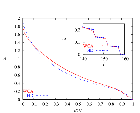
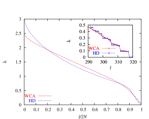
Figure 1: Lyapunov spectra for soft (WCA) and hard (HD) disks at low ($\rho=0.2$, upper panel) and intermediate ($\rho=0.4$, lower panel) densities. The very elongated rectangular simulation box is the same in both cases $(L_{x}=100,L_{y}=4,A=0.04),$ such that $N=80$ (top) and $N=160$ (bottom) disks are involved, respectively. The temperature $T=1$. The Lyapunov index $l$ is normalized by $2N$. Only the positive branches of the spectra are shown. Although the spectra are only defined for integer values of $l$, smooth lines are drawn for clarity. In the inset a magnified view of the small-exponents regime is shown, where $l$ is not normalized.

This general picture also persists for intermediate gas densities, $\rho=0.4,$ as shown in the lower panel of Fig. 1. The box size is the same as before, but the number of particles (and, as a consequence, also the number of exponents) is doubled. The spectral shapes for the WCA and hard-disk fluids, and the maximum exponents $\lambda_{1}$ in particular, become significantly different. Chaos, measured by $\lambda_{1}$, is obviously enhanced for the WCA particles with a finite collision time as compared to the instantaneously colliding hard disks. Interestingly, the Kolmogorov-Sinai (or dynamical) entropy $h_{KS}$, which is equal to the sum of all positive exponents Pesin ; ER85 , differs less due to the compensating effect of the intermediate exponents in the range $0.2<l/2N<0.8$. This may be verified in Fig. 4 below.

The systems of Fig. 1 are quasi one-dimensional and do not represent bulk fluids. We show in Fig. 2 analogous spectra for bulk systems in a rectangular simulation box with aspect ratio $A=0.6$, and containing $N=375$ particles. The density varies between 0.1 and 0.4 and is specified by the labels.

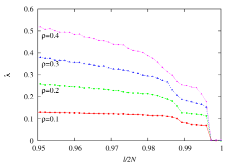
Figure 2: Lyapunov spectra for WCA-disk fluids with $N=375$ particles in a periodic box with fixed aspect ratio $A=0.6.$ Only the small exponents are shown as a function of the reduced index $l/2N$. The density is indicated by the labels.

For all spectra the lowest step is clearly discernible, but is progressively less pronounced if the density is increased. For $\rho=0.1$, the four smallest exponents $(744\leq l\leq 747)$ are identified as belonging to longitudinal modes (see below), the two next-larger exponents $(742\leq l\leq 743)$ to transverse modes. In Figure 3 we compare a WCA system to a hard-disk system in a square simulation box at a density $\rho=0.4$ and $N=400$ particles. The length of the simulation box in every direction is $L_{x}=L_{y}=31.62$. The step structure that is so prominent in the hard disk spectrum vanishes altogether for the soft potential case. If the density of such a square system with $N=400$ particles is reduced by increasing the size of the simulation box, the step structure with the same degeneracy reappears.

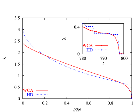
Figure 3: Lyapunov spectrum for WCA and hard-disk fluids with $N=400$ particles, a density $\rho=0.4$, and $L_{x}=L_{y}=31.62$. The temperature $T=1$. The Lyapunov index $l$ is normalized by $2N$. The inset shows the lower part of the spectra where the step structure is prominent for the hard disks but totally absent for the WCA particles. For this part, the index is not normalized.

III.2 Measures for chaos

The maximum Lyapunov exponent, $\lambda_{1}$, and the Kolmogorov-Sinai entropy, $h_{KS}$, are generally accepted as measures for chaos. The latter corresponds to the rate of information generated by the dynamics and, according to Pesin’s theorem Pesin ; ER85 is equal to the sum of the positive Lyapunov exponents, $h_{KS}=\sum_{\lambda_{l}>0}\lambda_{l}$. In Fig. 4 we compare the isothermal density dependences of these quantities for 375-disk WCA systems with corresponding hard-disk results. Also included in this set of figures is a comparison for the smallest positive exponent, $\lambda_{2N-3}$, which is directly affected by the mechanism generating the Lyapunov mode with the longest-possible wave length (if it exists).

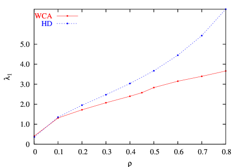
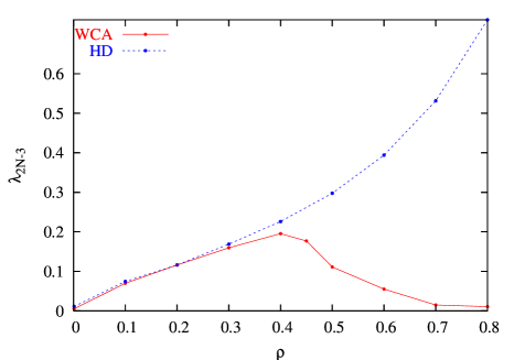
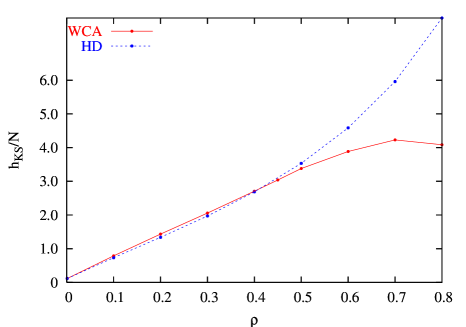
Figure 4: Isothermal density dependence of the maximum Lyapunov exponent, $\lambda_{1}$ (top), of the smallest positive exponent, $\lambda_{2N-3}$ (middle), and of the Kolmogorov-Sinai entropy per particle, $h_{KS}/N$ (bottom), for hard and soft-disk systems as a function of the density. The particle number, $N=375$, the aspect ratio, $A=0.6$, of the periodic box, and the temperature, $T=1$ are held fixed.

For very dilute hard-disk gases, $\lambda_{1}$ and $h_{KS}/N$ have been estimated from kinetic theory by Dorfman, van Beijeren and van Zon Szasz , who have provided expansions to leading orders in $\rho$, $\lambda_{1}=A\rho(-\ln\rho+B)+\dots$, and $h_{KS}/N=\bar{A}\rho(-\ln\rho+\bar{B})+\dots$, with explicit expressions for the constants $A,B$ and $\bar{A},\bar{B}$. These predictions were very successfully confirmed by computer simulations BDPD ; ZBD . Computer simulations by Dellago, Posch and Hoover also provided hard-disk results over the whole range of densities dph96 . $\lambda_{1}$ and $h_{KS}/N$ were found to increase monotonously with $\rho$ with the exception of a loop in the density range between the freezing point of the fluid ( $\rho_{f}=0.88$ Stillinger ) and the melting point of the solid ($\rho_{m}=0.91$ Stillinger ). These loops disappear if $\lambda_{1}$ and $h_{KS}/N$, are plotted as a function of the collision frequency $\nu$ instead of the density dph96 . If $\rho$ approaches the close-packed density $\rho_{0}=1.1547/\sigma^{2}$, both $\lambda_{1}$ and $h_{KS}/N$ diverge as a consequence of the divergence of $\nu$.

The results for the WCA disks reported here are for $0.1\leq\rho\leq 0.8$, which covers almost the whole fluid range. Simulations for rarefied gases and for solids are currently under way Forster05 . Not unexpectedly, we infer from the top panel of Fig. 4 that $\lambda_{1}$-WCA approaches $\lambda_{1}$-HD for small densities $\rho<0.1$. However, The density dependence for larger $\rho$ is qualitatively different. $\lambda_{1}$ approaches a maximum near the density corresponding to the fluid-to-solid phase transition, which confirms our previous results for Lennard-Jones fluids and solids Bunsen . The collective dynamics at such a transition causes maximum chaos in phase space. In the solid regime (not included in Fig. 4) $\lambda_{1}$ drops with increasing density, which is easily understandable.

The smallest positive exponent $\lambda_{2N-3}$ for soft-disk gases follows the hard-disk density behavior more closely than $\lambda_{1}$ for lower densities as inferred from the middle panel of Fig. 4. This means that the associated collective dynamics is affected less by the details of the pair potential. Significant deviations start to occur for $\rho>0.3$. For $h_{KS}/N$ the agreement between soft and hard disks extends even to a larger range of densities, as may be seen in the bottom panel of Fig. 4. However, this observation is deceptive and does not necessarily signal a similar dynamics. It is a consequence of significant cancellation due to the exponents intermediate between the maximum and the small exponents of the spectra such as in the bottom panel of Fig. 1.

III.3 Localization of tangent-space perturbations in physical space

One may interpret the maximum (minimum) Lyapunov exponent as the rate constant for the fastest growth (decay) of a phase-space perturbation. Thus, it is dominated by the fastest dynamical events, binary collisions in the case of particle fluids. Therefore, it does not come as a surprise that the associated tangent vector has components which are strongly localized in physical space mph98 . Similar observations for other spatially-extended systems have been made before by various authors Manneville:1985 ; Livi:1989 ; Giacomelli:1991 ; Falcioni:1991 . With the help of a particular measure for the localizationMilanovic:2002 , we could show that for both hard and soft disk systems the localization persists even in the thermodynamic limit, such that the fraction of tangent-vector components contributing to the generation of $\lambda_{1}$ at any instant of time converges to zero with $N\to\infty$ fhph04 ; pf04 . The localization becomes gradually worse for larger Lyapunov indices $l>1$, until it ceases to exist and (almost) all particles collectively contribute to the perturbations associated with the smallest Lyapunov exponents, for which coherent modes are known (or believed) to exist fhph04 ; pf04 .

Here, we adopt another entropy-based localization measure due to Taniguchi and Morriss Morriss:2003 which was successfully applied to quasi-onedimensional hard-disk gases. Recalling the definition of the individual particle contributions $\gamma_{i}^{(l)}$ to $\delta_{l}^{2}(\equiv 1)$ in Eq. (7), one may introduce an entropy-like quantity

$$S^{(l)}=-\sum_{i=1}^{N}{\langle\gamma_{i}^{(l)}(t)\ln\gamma_{i}^{(l)}(t)\rangle}\;,$$ (8)

where $\langle\dots\rangle$ denotes a time average. The number

$$W^{(l)}\equiv\exp\left(S^{(l)}\right)$$ (9)

may be taken as a measure for the spatial localization of the perturbation $\delta_{l}$ associated with $\lambda_{l}$, $1\leq l\leq 2N$. It is bounded according to $1\leq W^{(l)}\leq N$. The lower bound, $1$, indicates the most-localized state with only one particle contributing, and the upper bound $N$ signals uniform contributions by all of the particles $\{\gamma_{i}^{(l)}=1/N,i=1,\dots,N\}.$ We shall refer to the set of normalized localization parameters $\{W^{(l)}/N,l=1,\dots,2N\}$ as the localization spectrum.

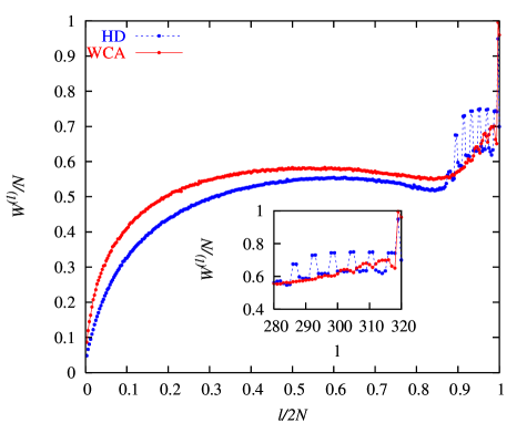
Figure 5: Dependence of the normalized localization parameters, $W^{(l)}/N$, on the normalized Lyapunov index $l/2N$. The corresponding Lyapunov spectra are shown in Fig. 1. The soft and hard disks are indicated by the labels and distinguished by color. The system is a rectangular box ($L_{x}=100$, $L_{y}=4$) with periodic boundaries. Top: $\rho=0.2$, $N=80$. Bottom: $\rho=0.4$, $N=160$. The temperature $T=1$. The insets provide a magnified view of the mode regime.

In Fig. 5 we compare the localization spectra for the same hard-disk and soft-disk systems for which the Lyapunov spectra are given in Fig. 1 ($L_{x}=100$, $L_{y}=4$, $A=0.04).$ For the lower-density gases in the top panel ($\rho=0.2$, $N=80$), the localization spectra for soft and hard disks are almost indistinguishable. They indicate strong localization for the perturbations belonging to the large exponents (small $l$), and collective behavior for large $l$. Of particular interest is the comb-like structure also magnified in the inset, which is a consequence of the Lyapunov modes (which will be discussed in more detail below). Stationary transverse modes are hardly affected by the time averaging involved in the computation of the localization measure and lead to large values of $W^{(l)}/N$, indicating strong collectivity. The propagating LP-modes EFPZ04 , however, are characterized by a significantly-reduced value of $W^{(l)}/N$. For intermediate gas densities in the bottom panel ($\rho=0.4$, $N=160$), differences between the hard and soft-disk results become apparent. Most prominently, the comb structure in the localization spectrum of the WCA system has mostly disappeared, although the Lyapunov spectrum clearly displays steps in the small-exponent regime, which is a clear indication for the existence of modes.

IV Zero modes

The dynamics in phase space and tangent space is strongly affected by the inherent symmetries of a system, i. e. infinitesimal transformations leaving the equations of motion invariant. They are intimately connected with the conservation laws obeyed by the dynamics. If these transformations act as infinitesimal perturbations of the initial conditions, the latter do not grow/shrink exponentially (but at most linearly) with time and give rise to as many vanishing Lyapunov exponents. The generators of these transformations are taken as unit vectors in tangent space, which point into the direction of the respective perturbation and are called zero modes. They span an invariant subspace ${\cal N}(\Gamma)$ of the tangent space at any phase point $\Gamma$, which is referred to as the zero subspace. They are essential for an understanding of the Lyapunov modes dealt with in the following.

For a planar system of hard or soft disks, there are six symmetry-related perturbations leading to non-exponential growth EFPZ04 ; WB04 and, hence, six vanishing Lyapunov exponents:

1. Homogeneous translation in $x$ and $y$ directions, with generators $e_{1}$ and $e_{2}$ explicitly given below. It is a consequence of center-of-mass conservation, which is actually not obeyed for systems with periodic boundary conditions, but, nevertheless, still holds for the linearized motion in tangent space, which does not recognize periodic box boundaries for the dynamics of the perturbations.

2. Homogeneous momentum perturbation in $x$ and $y$ directions due to Galilei invariance, with generators $e_{3}$ and $e_{4}$ given below. It may be viewed as a consequence of momentum conservation.

3. Simultaneous momentum and force rescaling according to a generator $e_{5}$ as given below. It is a consequence of energy conservation and, ultimately, of the homogeneity of time.

4. Homogeneous time shift with generator $e_{6}$, corresponding to non-exponential growth in the direction of the phase flow and also a consequence of the homogeneity of time.

These generators follow from the constraints the conservation equations impose on the dynamics in phase space. The latter constitute hyper-surfaces, $\sum_{i=1}^{N}x_{i}=$ const, $\sum_{i=1}^{N}y_{i}$= const for the center of mass (see the comment above), $\sum_{i=1}^{N}p_{x,i}=0$, $\sum_{i=1}^{N}p_{y,i}=0$ for the conserved momentum, and $\sum_{i=1}^{N}(p_{x,i}^{2}+p_{y,i}^{2})/2+\Phi=E$ for the conserved energy. The gradients perpendicular to these hyper-surfaces provide directions of non-exponential phase-space growth and, hence, the generating vectors $e_{1},\dots,e_{5}$ If we use the explicit notation

$$\delta\Gamma=\{\delta x_{i},\delta y_{i},\delta p_{x,i},\delta p_{y,i};i=1,\dots,N\}$$

for an arbitrary tangent vector, one obtains

$$e_{1} = (1/N)\{1,0,0,0;i=1,\dots,N\}$$ (10)

$$e_{2} = (1/N)\{0,1,0,0;i=1,\dots,N\}$$ (11)

$$e_{3} = (1/N)\{0,0,1,0;i=1,\dots,N\}$$ (12)

$$e_{4} = (1/N)\{0,0,0,1;i=1,\dots,N\}$$ (13)

$$e_{5} = \alpha\{-F_{x,i},-F_{y,i},p_{x,i},p_{y,i};i=1,\dots,N\}$$ (14)

$$e_{6} = \alpha\{p_{x,i},p_{y,i},;F_{x,i},F_{y,i};i=1,\dots,N\},$$ (15)

where $\alpha$ is a normalizing factor. Each vector has $4N$ dimensions. $e_{1}$ to $e_{6}$ are orthonormal and form a natural basis for the invariant zero space. In the following we consider the expansion of the six orthonormal tangent vectors $\delta_{2N-2},\dots,\delta_{2N+3}$, responsible for the six vanishing exponents in the simulation, in that basis,

$$\delta_{2N-3+l}=\sum_{j=1}^{6}\alpha_{l,j}\;e_{j}\;,\;l=1,\dots,6\;,$$ (16)

with projection cosines, $\alpha_{l,j}\equiv(\delta_{l}\cdot e_{j})$. Since all vectors involved are of unit length, $\alpha_{l,j}$ may either be interpreted as the projection of $\delta_{2N-3+l}$ onto $e_{j}$, or vice versa.

For hard disk fluids one can easily show EFPZ04 that the tangent vectors $\delta_{2N-2},\dots,\delta_{2N+3}$ are fully contained in ${\cal N}(\Gamma)$. The projection cosines strictly obey the sum rules

$$\sum_{i=1}^{6}(\alpha_{l,i})^{2}=1\;\;\;,\;\;\;\sum_{l=1}^{6}(\alpha_{l,i})^{2}=1\;,$$

at all times, if the total momentum vanishes and if $K=N$, as is always the case in our simulations. Thus, ${\rm Span}(\delta_{2N-2},\dots,\delta_{2N+3})={\rm Span}(e_{1},\dots,e_{6}).$ Note that there are no forces acting on the particles in this case, and the particles are moving on straight lines between successive instantaneous collisions.

For soft disk systems, however, the situation is more complicated.

Table 1: Projection cosines, $\alpha_{l,j}$, according to Eq. (16) for $N=4$ soft particles in a periodic box and interacting with the power-law potential (2). The density is low, $\rho=0.1$, to isolate individual collision events. Two instants are considered:

A: At time $t_{0}$ just before a collision of particles 1 and 2:

$l$	$\alpha_{l,1}$	$\alpha_{l,2}$	$\alpha_{l,3}$	$\alpha_{l,4}$	$\alpha_{l,5}$	$\alpha_{l,6}$	$\sum_{j=1}^{6}{(\alpha_{l,j})^{2}}$
1	-1.00000	0.00000	0.00000	0.00000	0.00000	0.00000	1.00000
2	0.00000	0.21120	0.00000	0.00000	-0.00001	-0.97734	0.99980
3	0.00000	0.97744	0.00000	0.00000	0.00000	0.21118	0.99999
4	0.00000	0.00000	0.95954	0.00000	0.28155	0.00000	0.99998
5	0.00000	0.00000	0.28158	0.00000	-0.95944	0.00001	${\it 0.99981}$
6	0.00000	0.00000	0.00000	1.00000	0.00000	0.00000	1.00000
$\sum_{l=1}^{6}{(\alpha_{l,j})^{2}}$	1.00000	1.00000	1.00000	1.00000	${\it 0.99979}$	${\it 0.99979}$

B: At time $t_{0}+0.11$ of closest approach of particles 1 and 2:

$l$	$\alpha_{l,1}$	$\alpha_{l,2}$	$\alpha_{l,3}$	$\alpha_{l,4}$	$\alpha_{l,5}$	$\alpha_{l,6}$	$\sum_{j=1}^{6}{(\alpha_{l,j})^{2}}$
1	-1.00000	0.00000	0.00000	0.00000	0.00000	0.00000	1.00000
2	0.00000	0.14132	0.00000	0.00000	0.00000	-0.08601	0.02737
3	0.00000	0.98996	0.00000	0.00000	0.00000	0.01228	0.98018
4	0.00000	0.00000	0.98172	0.00000	0.01654	0.00000	0.96405
5	0.00000	0.00000	0.19033	0.00000	-0.08529	0.00000	${\it 0.04350}$
6	0.00000	0.00000	0.00000	1.00000	0.00000	0.00000	1.00000
$\sum_{l=1}^{6}{(\alpha_{l,j})^{2}}$	1.00000	1.00000	1.00000	1.00000	${\it 0.00755}$	${\it 0.00755}$

In Table 1 we list instantaneous matrix elements $\alpha_{l,j}$ for a simple example, $N=4$ particles interacting with the particularly-smooth repulsive potential of Eq. 2. The density, $\rho=0.1$, is low enough such that isolated binary collisions may be easily identified. Two instances are considered: one just at the beginning of a collision of particles 1 and 2 (upper part of the table), and a time half way through this collision (lower part of the table). Considering the columns first, the squared sums $\sum_{l=1}^{6}{(\alpha_{l,j})^{2}}$ always add to unity for $j=1,\dots,4$, which means that $e_{1}$ to $e_{4}$ are fully contained in the subspace ${\rm Span}(\delta_{2N-2},\dots,\delta_{2N+3})$ of the tangent space. The same is not true, however, for $e_{5}$ and $e_{6}$, which contain in their definition the instantaneous forces acting on the colliding particles. If no collisions take place anywhere in the system (upper part), the subspaces ${\rm Span}(\delta_{2N-2},\dots,\delta_{2N+3})$ and ${\rm Span}(e_{1},\dots,e_{6})$ are nearly the same, but not quite, as the squared projection-cosine sums indicate. The moment a collision occurs, the sums $\sum_{l=1}^{6}{(\alpha_{l,j})^{2}}$ for $j=5$ and $6$ may almost vanish, as happens in the bottom part of the table, and the vectors $e_{5}$ and $e_{6}$ become nearly orthogonal to ${\rm Span}(\delta_{2N-2},\dots,\delta_{2N+3})$. In Figure 6

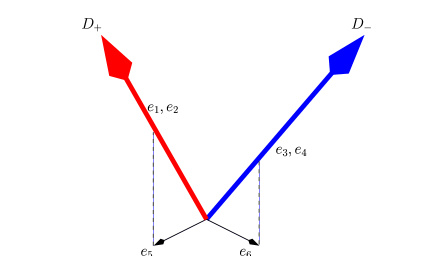
Figure 6: Caricature of the high-dimensional tangent space for $N$ particles. The orthogonal zero modes $e_{1}$ and $e_{2}$ always point into the subspace ${\cal D}_{+}\equiv{\rm Span}(\delta_{2N-2},\delta_{2N-1},\delta_{2N})$. Similarly, the zero modes $e_{3}$ and $e_{4}$ always point into the subspace ${\cal D}_{-}\equiv{\rm Span}(\delta_{2N+1},\delta_{2N+2},\delta_{2N+3})$. The subspaces ${\cal D}_{+}$ and ${\cal D}_{-}$ are represented by the thick arrows. The projection angle of the zero mode $e_{5}$ into ${\cal D}_{+}$ agrees with that of $e_{6}$ into ${\cal D}_{-}$ and generally differs from zero whenever a collision occurs anywhere in the system.

an attempt is made to illustrate this relationship for such a high-dimensional tangent space. For systems containing many particles and/or for larger densities, there will always be at least one collision in progress, and the horizontal sums, $\sum_{j=1}^{6}{(\alpha_{l,j})^{2}}$ for $l=1,\dots,6$, and the vertical sums, $\sum_{l=1}^{6}{(\alpha_{l,j})^{2}}$ for $j=5$ and $6$, fluctuate and assume values significantly smaller than unity. The subspaces ${\rm Span}(\delta_{2N-2},\dots,\delta_{2N+3})$ = ${\cal D}_{+}\oplus{\cal D}_{-}$ (see the definition in Fig. 6) and ${\cal N}={\rm Span}(e_{1},\dots,e_{6})$ do not agree in general.

V Lyapunov modes

Lyapunov modes are periodic spatial patterns observed for the perturbations associated with the small positive and negative Lyapunov exponents. They are characterized by wave vectors $k$ with wave number

$$k_{n_{x},n_{y}}=\sqrt{\left({\frac{2\pi}{L_{x}}}\,n_{x}\right)^{2}+\left({\frac{2\pi}{L_{y}}}\,n_{y}\right)^{2}}\;;\;\;n_{x},n_{y}=0,1,\ldots\;\;,$$ (17)

where a rectangular box with periodic boundaries is assumed, and where $n_{x}$ and $n_{y}$ denote the number of nodes parallel to $x$ and $y$, respectively. For modifications due to other boundary conditions we refer to Refs. EFPZ04 ; TM03 . Experimentally, Lyapunov modes were observed for hard particle systems in one, two, and three dimensions mathII ; hpfdz02 ; EFPZ04 ; Morriss:2003 ; Morriss:2004 , for hard planar dumbbells mph98 ; mph98a ; Milanovic:2002 , and, most recently, for one-dimensional soft particles ry04a ; ry04b . Theoretically, they are interpreted as periodic modulations $(k\neq 0)$ of the zero modes, to which they converge for $k\to 0$. Since a modulation, for $k>0$, involves the breaking of a continuous symmetry (translational symmetry of the zero modes), they have been identified as Goldstone modes WB04 , analogous to the familiar hydrodynamic modes and phonons. For the computation of the associated wave-vector dependent Lyapunov exponents governing the exponential time evolution of the Lyapunov modes, random matrices eg00 ; TM02 , periodic-orbit expansion TDM02 , and, most successfully, kinetic theory have been employed WB04 ; MM01 ; MM04 .

For hard-disk systems the representation of the modes is simplified by the fact that, for large $N$, the position perturbations, $\{\delta q_{i}^{(l)},i=1,\dots,N\}$, and momentum perturbations, $\{\delta p_{i}^{(l)},i=1,\dots,N\}$, may be viewed as two-dimensional vector fields $\varphi_{q}^{(l)}(x,y)$ and $\varphi_{p}^{(l)}(x,y)$, respectively, which turn out to be nearly parallel (for $\lambda>0$), or anti-parallel (for $\lambda<0$) EFPZ04 . To illustrate this point, we plot in Fig. 7

$$\left\langle\cos(\Theta_{l})\right\rangle\equiv\left\langle\frac{\sum_{i=1}^{N}(\delta q_{i}^{(l)}\cdot\delta p_{i}^{(l)})}{\sum_{i=1}^{N}(\delta q_{i}^{(l)})^{2}\sum_{i=1}^{N}(\delta p_{i}^{(l)})^{2}}\right\rangle,$$ (18)

where $\Theta_{l}$ is the angle between the $2N$-dimensional vectors comprising the position and momentum perturbations of $\delta_{l}$, when they are viewed in the same $2N$-dimensional space. As always, $\langle\dots\rangle$ denotes a time average. Only the indices $l<2N-2$ corresponding to positive exponents are considered. $\Theta_{l}$ (upper blue curve) nearly vanishes in the mode regime (close to the right-hand boundary of that figure). For the negative exponents (not shown) the angle approaches $\pi$. For large-enough $N$ and small positive $\lambda_{l}$, the individual particle contributions behave as

$$\delta p_{i}^{(l)}=C_{i}^{(l)}(\Gamma)\delta q_{i}^{(l)},$$

where $C_{i}^{(l)}$ is a positive number, which is almost the same for all particles $i$. Once the $\delta q_{i}^{(l)}$ are known, the $\delta p_{i}^{(l)}$ may be obtained from this relation. For a characterization of the modes, it suffices to consider only the position perturbations, which are interpreted as a vector field, $\varphi_{q}^{(l)}(x,y)$, over the simulation cell EFPZ04 .

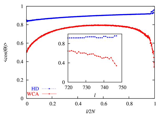
Figure 7: Time-averaged values for $\cos(\Theta_{l})$, as defined in Eq. (18), for the indices $1\leq l\leq 2N-3$ corresponding to the positive Lyapunov exponents of a spectrum. The systems consist of N = 375 particles at a density $\rho=0.4$ in a rectangular periodic box with aspect ratio $A=0.6$; Upper blue points: hard disks (HD); Lower red points: soft WCA disks. In both cases, the temperature is unity.

For soft-spheres the situation is more complicated. For low-density systems, $\cos(\Theta_{l})$ behaves as for hard disks, which is expected in view of the similarity of the Lyapunov spectra. For dense fluids, however, this quantity behaves qualitatively different and does not converge to unity but to zero in the interesting mode regime. This is demonstrated in Fig. 7 by the lower red curve, which is for $N=375$ soft WCA disks at the same density $\rho=0.4$. The larger the collision frequency, the larger the deviations of $\langle\cos(\Theta_{l})\rangle$ from 1 (for $\lambda_{l}>0$), or -1 (for $\lambda_{l}<0$) may become. This result indicates that a representation of a Lyapunov mode in terms of a single (periodic) vector field of the position (or momentum) perturbations of the particles is possible only for low-density systems. For larger densities and/or larger systems with many collisional events taking place at the same time, one needs to simultaneously consider all the perturbation components $\delta x_{i},\delta y_{i},\delta p_{x,i},\delta p_{y,i}$ of a particle.

To understand this unexpected behavior in more detail, we display in the top panel of Fig. 8 the time dependences of $\cos(\Theta_{l})$ belonging to the maximum $(l=1)$ and to the smallest-positive $(l=2N-3=5)$ exponents of a four-particle system in a square periodic box with a density $\rho=0.1$. During a streaming phase without collisions, the $2N$-dimensional vectors $\delta q^{(l)}$ and $\delta p^{(l)}$ tend to become parallel as required by the linearized free-flight equations in tangent space. However, this process is disrupted by a collision, which reduces (and in some cases even reverses the sign of) $\cos(\Theta_{l})$. In the following streaming phase, i.e. forward in time, $\Theta_{l}(t)$ relaxes towards zero. This suggests that the numerical time evolution of $\cos(\Theta_{l})$ and, hence, of $\delta_{l}$ is not invariant with respect to time reversal. This is indeed the case as is demonstrated in the lower panel of Fig. 8. To construct this figure, the phase space trajectory was stored for another 10000 time units and, after a time-reversal transformation, $\{q_{i}\to q_{i},p_{i}\to-p_{i};i=1,\dots,N\}$, was consecutively used - in reversed order - as the reference trajectory for the reversed tangent-space dynamics. In the lower panel we show $\cos(\Theta_{16})$ and $\cos(\Theta_{12})$, which belong to the minimum and largest-negative exponents, of the time-reversed dynamics, respectively, and which should be compared to $\cos(\Theta_{1})$ and $\cos(\Theta_{5})$ for the forward evolution. Although the same collisions are involved, the curves look totally different. This confirms previous results concerning the lack of symmetry for the forward and backward time evolution of the Gram-Schmidt orthonormalized tangent vectors $\delta_{l}$ for Lyapunov-unstable systems HHP01 ; HPH01 . Furthermore, we have numerically verified that $\cos(\Theta_{l}(t))=\cos(\Theta_{4N-l+1}(t))$ is always obeyed, both forward and backward in time.

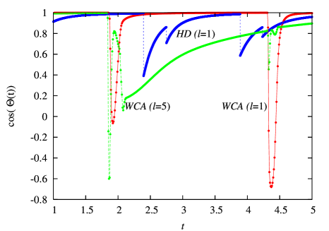
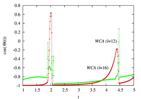
Figure 8: Time dependence of $\cos(\Theta_{l})$ both in the time-forward (upper panel) and time-backward directions (lower panel) for four WCA particles in a square periodic box. The density $\rho=0.1$. The respective indices, $l$, are indicated by the labels. For comparison, an analogous hard-disk result for $l=1$ is also shown by the blue curve in the upper panel.

VI Fourier-transform analysis

Because of numerical fluctuations, a simple inspection of the vector field $\varphi_{q}^{(l)}(x,y)$ very often is not sufficient to unambiguously determine the wave vector of a mode, particularly for the smaller than the maximum-possible wave lengths. Therefore, Fourier transformation methods have been used Forster:2004 , where we regard $\varphi_{a}(x,y)$ as a spatial distribution

$$\chi_{a}(q)=\sum_{i=1}^{N}a_{i}\delta(q-q_{i}).$$ (19)

The $a_{i}$ are identified, for example, with $\delta x_{i}^{(l)}$ or with
$\left(\gamma_{i}^{(l)}\right)^{1/2}\equiv\left((\delta x_{i}^{(l)})^{2}+(\delta y_{i}^{(l)})^{2}+(\delta p_{x,i}^{(l)})^{2}+(\delta p_{y,i}^{(l)})^{2}\right)^{1/2}$. In view of the periodicity of the box, the Fourier coefficients have wave numbers given by Eq. (17). They are computed from

$$\chi_{a}({k})\equiv\frac{1}{L_{x}L_{y}}\int d^{2}qe^{k\cdot q}\chi_{a}(q)=\frac{1}{L_{x}L_{y}}\sum_{i}a_{i}e^{k\cdot q_{i}}.$$ (20)

The power spectrum is defined by

$$P_{a}({k})=\chi_{a}({k})\chi_{a}({-k}).$$ (21)

For the $a_{i}$ identified above, the power spectra are denoted by $P_{x}(k)$ and $P_{\gamma^{1/2}}(k)$, respectively. We have also applied the algorithm for unequally-spaced points by Lomb Lomb:1976 ; recipes , suitably generalized to two-dimensional transforms.

As a first example we show in Figure 9 the power spectra $P_{\gamma^{1/2}}(k)$ for successive transverse modes, indexed by $l=317$, 311, 305, 299, 293, and 287, for the WCA-system described in the lower panel of Fig. 1. They

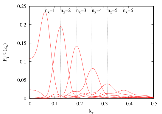
Figure 9: Power spectra $P_{qp}(k)$ for the transverse modes T(1,0) to T(6,0) with $l=317$, 311, 305, 299, 293, and 287, for $N=160$ WCA particles in an elongated periodic box, $L_{x}=100,L_{y}=4$. The density $\rho=0.4.$ The Lyapunov spectrum for this system is shown in the lower panel of Fig. 1.

correspond to the successive wave numbers $k_{1,0}$ to $k_{6,0}$ as predicted by Eq. (17). In a second and less-trivial example, we show in Fig. 10 the Lyapunov spectra (left panel) of WCA particles in a fixed elongated box, $L_{x}=100,L_{y}=4$, for various densities varying from $\rho=0.1$ to $\rho=0.7$ as indicated by the labels.

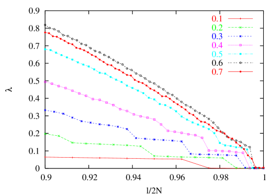
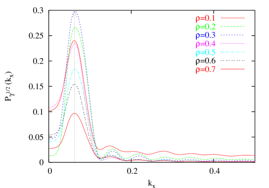
Figure 10: WCA particles in a fixed periodic box, $L_{x}=100,L_{y}=4$, for various densities as indicated by the labels. The temperature is unity. Upper panel: Lyapunov spectra, plotted with a reduced index $l/2N$ on the abscissa; Lower panel: power spectra $P_{\gamma^{1/2}}(k)$ for the modes corresponding to the smallest positive exponent, $\lambda_{l=2N-3}$, of each spectrum.

In the right panel the power spectra $P_{\gamma^{1/2}}(k)$ for the modes corresponding to the smallest positive exponent, $\lambda_{l=2N-3}$, of each spectrum are shown. Since $L_{x}$ is the same in all cases, all power spectra have a peak at the allowed wave number $k_{1,0}=0.063$. This peak is also well resolved for large densities, for which the step structure in the spectrum is blurred.

VII Concluding remarks

In the foregoing sections we have demonstrated the existence of Lyapunov modes in soft-disk fluids with the help of various indicators such as the localization measure in Sec. III.3, and the Fourier analysis in the previous section. However, the classification and characterization of the modes is more complicated than for hard disks. This is demonstrated in Fig. 11, where the position perturbations $\delta x_{i}^{746}$ (bottom) and $\delta y_{i}^{746}$ (top) are plotted at the particle positions in the simulation cell for the 375-particle system with a density $\rho=0.4$ familiar from Fig. 2. Naively, the upper surface

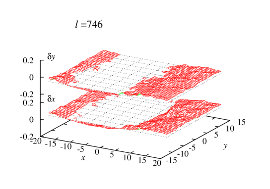
Figure 11: Representation of a Lyapunov mode as periodic spatial patterns of the position perturbations $\delta x_{i}$ and $\delta y_{i}$ of the particles in the periodic box. The system consists of 375 WCA disks at a density $\rho=0.4$ in a rectangular box with an aspect ratio $A=0.6$. The Lyapunov spectrum for this system is given by the top-most curve of Fig. 2. The mode $l=746$ is shown.

would have to be classified as a transverse mode with the perturbation component $\delta y$ perpendicular to a wave vector $k$ parallel to $x$, and the lower surface as a longitudinal mode with $\delta x$ parallel to $k$. Since the momentum perturbations are not nearly as parallel to the position perturbations (see Fig. 7) as is (approximately) the case for hard disks, it is not sufficient to represent a mode by a single two-dimensional vector field such as $\varphi_{q}^{(l)}(x,y)$ or $\varphi_{p}^{(l)}(x,y)$. Position and momentum perturbations need to be considered simultaneously for a characterization of the modes. The disappearance of the step structure in the Lyapunov spectrum and, hence, of the degeneracy for larger densities points to a complicated tangent-space dynamics we have not yet been able to unravel. We do not know of any theory which accounts for all of the numerical results presented in this paper.

References

- [1] B.J. Alder and T.E. Wainwright, Scientific American, 201, 113, (1959).
- [2] H.A. Posch and Wm.G. Hoover, Phys. Rev. A, 38, 473–482, (1988).
- [3] B. L. Holian, W.G. Hoover and H. A. Posch, Phys. Rev. Lett. 59, 10 - 13 (1987).
- [4] Lj. Milanovi’c, H. A. Posch, and Wm. G. Hoover, Molec. Phys. 95, 281 (1998).
- [5] H. A. Posch, unpublished.
- [6] J.D. Bernal and S.V King, in Physics of Simple Liquids, edited by H.N.V. Temperley, (North-Holland, Amsterdam, 1968).
- [7] J.-P. Hansen and I.R. McDonald, in Theory of simple liquids, (Academic Press, London, 1991).
- [8] T.M. Reed and K.E. Gubbins, in Applied Statistical Mechanics, (McGraw Hill, Tokyo, 1973).
- [9] H.A. Posch and R. Hirschl, in Hard Ball Systems and the Lorentz Gas, p. 279, edited by D. Szasz, Encyclopedia of Mathematical Sciences, vol. 101, (Springer Verlag, Berlin, 2002).
- [10] H.A. Posch and Ch. Forster, in Lecture Notes on Computational Science - ICCS 2002, p. 1170, edited by P.M.A Sloot, C.J.K Tan, J.J. Dongarra, and A.G. Hoekstra, (Springer Verlag, Berlin, 2002).
- [11] Wm.G. Hoover, H.A. Posch, Ch. Forster, Ch. Dellago, and M. Zhou, Journal of Statistical Physics, 109,765–776, (2002).
- [12] Lj. Milanović and H.A. Posch, J. Molec. Liquids, 96-97, 221 (2002).
- [13] J.-P. Eckmann, Ch. Forster, H.A. Posch, and E. Zabey, J. of Stat. Phys., submitted (2004).
- [14] J.-P. Eckmann and O. Gat, J. Stat. Phys. 98, 775 (2000).
- [15] S. McNamara and M. Mareschal, Phys. Rev. E64, 051103 (2001).
- [16] M. Mareschal and S. McNamara, Physica D, 187, 311 (2004).
- [17] A. de Wijn and H. van Beijeren, Phys. Rev. E , 70, 016207 (2004).
- [18] T. Taniguchi and G. P. Morriss, arXiv: nlin.CD/0404052, submitted (2004).
- [19] Ch. Dellago, Wm.G. Hoover and H.A. Posch, Physical Review E, 65, (2002)
- [20] G. Radons and H. Yang, Phys. Rev. Lett, submitted (2004).
- [21] H. Yang and G. Radons, Phys. Rev. E, submitted (2004).
- [22] G. Benettin, L. Galgani, A. Giorgilli, and J.M. Sterilizing, Meccanica, 15, 29, (1980).
- [23] I. Shimada and T. Nagasihma, Prog. Theor. Phys, 61, 1605, (1979).
- [24] V.I. Oseledec, Trans. Mosc. Math. Soc, 19, 197, (1968).
- [25] Ch. Dellago, H. A. Posch, and Wm. G. Hoover, Phys. Rev. E, 53, 1485, (1996).
- [26] Ch. Dellago and H. A. Posch, Physica A 240, 68 (1997).
- [27] D.J. Evans and E.G.D. Cohen and G.P. Morris, Physical Review A, 42,5990, (1990).
- [28] D. Ruelle, Journal of Stat. Physics, 95,393, (1999).
- [29] F.J. Lingen, Communications in numerical methods in engineering, 16,57-66 (2000)
- [30] T. Taniguchi and G.P. Morris, Phys. Rev. E, 65, 056202 (2002).
- [31] Ch. Forster, R. Hirschl, H. A. Posch, and Wm.G. Hoover, Physica D, 187, 294, 2004.
- [32] Ya. B. Pesin, Usp. Mat. Nauk 32, No. 4, 55 (1977) [Russian Math. Survey 32, No. 4, 55 (1977)].
- [33] J.-P. Eckmann and D. Ruelle, Rev. of Mod. Physics, 57, 617 (1985).
- [34] R. van Zon, H. van Beijeren, and J. R. Dorfman, in Hard Ball Systems and the Lorentz Gas, edited by D. Szasz, p. 231, Encyclopedia of Mathematical Sciences, vol. 101, (Springer Verlag, Berlin, 2000). This paper contains also a comprehensive list of references to previous work of the same authors.
- [35] H. van Beijeren, J. R. Dorfman, H. A. Posch, and Ch. Dellago, Phys. Rev. E, 56, 5272 (1997).
- [36] R. van Zon, H. van Beijeren, and C. Dellago, Phys. Rev. Lett. 80, 2053 (1998).
- [37] T. M. Truskett, S. Torquato, S. Sastry, P. G. Debenedetti, and F. H. Stillinger, Phys. Rev. E, 58, 3083 (1998).
- [38] Ch. Forster and H. A. Posch, unpublished.
- [39] H. A. Posch, Wm. G. Hoover, and B. L. Holian, Ber. Bunsenges. Phys. Chem. 94, 250 (1990).
- [40] P. Manneville, Lect. Notes Phys. 230, 319 (1985).
- [41] R. Livi and S. Ruffo, in Nonlinear Dynamics, edited by G. Turchetti (World Scientific, Singapore, 1989), p. 220.
- [42] G. Gacomelli and A. Politi, Europhys. Lett., 15,387, (1991)
- [43] M. Falcioni, U.M.B. Marconi and A. Vulpiani, Phy. Rev. A, 44, 2263, (1991)
- [44] T. Taniguchi and G. P. Morriss, Phy. Rev. E, 68, 046203, (2003).
- [45] T. Taniguchi and G. P. Morriss, Phy. Rev. E, 68, 026218, (2003).
- [46] Lj. Milanovi’c, H.A. Posch, and Wm. G. Hoover, Chaos. 8, 455 (1998).
- [47] T. Taniguchi, C.P. Dettmann, and G.P. Morriss, J. Stat. Phys. 109, 747 (2002).
- [48] Wm. G. Hoover, C. G. Hoover, and H.A. Posch, Comput. Meth. Sci. Tech. 7, 55 (2001).
- [49] Wm. G. Hoover, H. A. Posch, and C. G. Hoover, J. Chem. Phys. 115, 5744 (2001).
- [50] Ch. Forster, R. Hirschl, and H. A. Posch, in Proceedings of the ICMP 2003, (World Scientific, Singapore, 2004).
- [51] N.R. Lomb, Astrophys. and Space Science, 39, 447 (1976).
- [52] W.H. Press, S.A. Teukolsky, W.T. Vetterling, B.P.Flannery, in Numerical Recipes in Fortran77: the Art of Scientific Computing, 2nd ed., (Cambridge University Press, Cambridge, 1999).