Universal decay of classical Loschmidt echo of neutrally stable but mixing dynamics

Abstract

We provide analytical and numerical evidence that classical mixing systems which lack exponential sensitivity on initial conditions, exhibit universal decay of Loschmidt echo which turns out to be a function of a single scaled time variable $\delta^{2/5}t$, where $\delta$ is the strength of perturbation. The role of dynamical instability and entropy production is discussed.

Fidelity, or Loschmidt echo, is defined as the overlap of two time evolving states which, starting from the same initial condition, evolve under two slightly different Hamiltonians. It is therefore an important quantity which measures the stability of the motion under system s perturbations. The recent interest in the behaviour of fidelity Peres ; Usaj ; Jalabert ; Prosen ; Beenakker ; Tomsovic ; PZ ; BC1 ; Eckhardt ; Veble ; VP has been largely motivated by a possible use in quantifying stability of quantum computation Qcomp .

It has been shown Veble that for classical chaotic, exponentially unstable systems, the decay rate of fidelity is perturbation independent and, asymptotically, fidelity decays as correlation functions. On the other hand, for quantum systems, fidelity decay obeys different regimes depending on perturbation strength. In this relation, particularly intriguing is the recently discovered case of mixing dynamics with vanishing Lyapounov exponent caspro99 ; caspro00 a prominent example of which are billiards inside polygons note . In several respects the classical dynamics of such systems is reminiscent of quantum dynamics of generic chaotic systems which, apart from an initial time, exponentially short in ${\hbar}$, are linearly stable. As a consequence statistical relaxation in quantum mechanics takes place in absence of exponential instability. Certainly, the dramatic difference in the dynamical stability properties of different systems must be reflected in a different qualitative behaviour of physical quantities such as fidelity which is the object of the present paper.

In the following, under the assumptions of linear separation of trajectories and dynamical mixing, which may be produced by some discontinuity in the flow, we derive a universal scaling law of classical fidelity decay. We conjecture that this surprising fidelity decay may be associated to a peculiar power-logarithmic entropy production in such systems. We consider here a specific example, i.e. the triangle map $z_{n+1}=T(z_{n})$ caspro00 on a torus $z=(x,y)\in[-1,1)\times[-1,1)$

$$y_{n+1} = y_{n}+\alpha{\rm\,sgn}x_{n}+\beta\pmod{2},$$

$$x_{n+1} = x_{n}+y_{n+1}\pmod{2},$$ (1)

where ${\rm sgn}x=\pm 1$ is the sign of $x$ and $\alpha,\beta$ are two parameters. Previous investigations have shown that caspro00 (see also mirko for some rigorous results on (1)): for rational values of $\alpha,\beta$ the system is pseudo-integrable, as the dynamics is confined on invariant curves. If $\alpha=0$ and $\beta$ is irrational, the dynamics is (uniquely) ergodic, but not mixing, while for incommensurate irrational values of $\alpha,\beta$ the dynamics is ergodic and mixing with dynamical correlation functions decaying as $t^{-3/2}$. It can be argued that the triangle map possesses the essential features of bounce maps of polygonal billiards and 1d hardpoint gases caspro99 ; caspro00 , namely parabolic stability in combination with decaying dynamical correlations, and as such represents a paradigmatic model for a larger class of systems.

The classical fidelity $F_{\delta}(n)$ can be written as an overlap of two phase space densities propagated by the original map $T$ and the perturbed map $T_{\delta}=T\circ g_{\delta}$ where $g_{\delta}(z)=z+\delta a(z)$ is some near-identity area-preserving map parametrized by a vector field $a(z)$:

$$F_{\delta}(n)=\frac{\int{\rm d}^{2}z\rho(T^{(-n)}(z))\rho(T^{(-n)}_{\delta}(z))}{\int{\rm d}^{2}z\rho^{2}(z)},$$ (2)

We can make our discussion even more general by taking the perturbation explicitly time-dependent. Let the perturbed map $T_{\delta,n}$ explicitly depend on iteration time, namely we consider the following class of perturbed triangle maps, $\bar{z}_{n+1}=T_{\delta,n}(\bar{z}_{n})$

$$\bar{y}_{n+1} = \bar{y}_{n}+\alpha{\rm\,sgn}\bar{x}_{n}+\beta+\delta f_{n}(\bar{x}_{n})\pmod{2},$$

$$\bar{x}_{n+1} = \bar{x}_{n}+\bar{y}_{n+1}\pmod{2}.$$ (3)

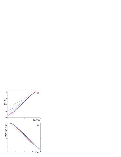
Figure 1: Fidelity decay. To compute fidelity we divide the phase space in $100\times 100$ cells. We then take $10^{5}$ points in one cell and evolve these points with the map (1) up to time $n$. Then we compute the reverse evolution with the map (3) and compute the fraction of points which fall again in the initial cell, after time $2n$. The result is then averaged over initial distributions in 49 different randomly chosen cells. (a) $\log(1-F_{\delta}(n))$ versus $\log(\delta^{2/5}n)$ magnifying behaviour for short times. The broken curves refer to $\delta=10^{-5},\ldots,10^{-10}$ (top-down). The full line is the theoretical expression (9). (b) $\log[(F_{\delta}(n)-u)/(1-u)]$ versus $\delta^{2/5}n$ magnifying asymptotic (long-time) behavior. Here $u=10^{-4}$ is the relative area of the initial set ${\cal A}$ giving the asymptotic value of fidelity. The meaning of broken curves is the same as in (a). The full curve gives the numerical solution of the random Gaussian model (12), while the dashed line has slope $-1$ to indicate asymptotic exponential decay.

We will assume that the force function $f_{n}$ has vanishing time-average for almost any initial condition. Let as further assume that the initial density $\rho(z)$ is a characteristic function over some set ${\cal A}$ of typical diameter $\omega$ with $\delta\ll\omega\ll 1$. Then a pair of orbits $z_{n}$ and $\bar{z}_{n}$ starting from the same point $\bar{z}_{0}=z_{0}$ in ${\cal A}$, contribute to (2) until they hit the opposite sides of the discontinuity, at $x=0,1\pmod{2}$. The fidelity at time $n$ is then simply the probability that the pair of orbits does not hit the cut up to $n-$th iterate. Assuming ergodicity of the map caspro00 we write

$$F_{\delta}(n)=\left\langle\prod_{n^{\prime}=1}^{n}(1-|\Delta x_{n^{\prime}}|)\right\rangle$$ (4)

where $\Delta x_{n}=\bar{x}_{n}-x_{n}$, and $\left\langle A_{n}\right\rangle=\int{\rm d}z\rho(z)A(T^{(n)}(z))/\int{\rm d}z\rho(z)$. In order to derive the fidelity decay for the triangle map we have to compute the average growth rate of the orbits distance perpendicular to the cut. This is achieved by writing out an explicit linearized map for the orbits displacement $\Delta z_{n}=\bar{z}_{n}-z_{n}$

$$\Delta z_{n+1}=\left(\begin{array}[]{cc}1&1\\ 0&1\\ \end{array}\right)\Delta z_{n}+\left(\begin{array}[]{c}1\\ 1\\ \end{array}\right)\delta f_{n}(x_{n}).$$ (5)

This system of linear difference equations can be solved explicitly, say for $\Delta x_{n}$:

$$\Delta x_{n}=\delta\sum_{n^{\prime}=0}^{n-1}(n-n^{\prime})f_{n^{\prime}}(x_{n^{\prime}})$$ (6)

with the initial condition $\Delta z_{0}=0$. Assuming that $f_{n}$ are pseudo-random variables with quickly decaying correlation function $C(n)=\lim_{m\to\infty}\left\langle f_{m}(x_{m})f_{n+m}(x_{n+m})\right\rangle$, we can employ a version of the central limit theorem to show that $\Delta x_{n}$ should have Gaussian distribution for sufficiently large $n$. To this end, let us first notice that the second moment

$$\left\langle(\Delta x_{n})^{2}\right\rangle=\delta^{2}\sum_{n^{\prime}=0}^{n-1}\sum_{n^{\prime\prime}=0}^{n-1}(n-n^{\prime})(n-n^{\prime\prime})\left\langle f_{n^{\prime}}f_{n^{\prime\prime}}\right\rangle$$ (7)

can be related, as $n\to\infty$, to the integrated correlation function. Since, for large $n$: $\left\langle f_{n^{\prime}}f_{n^{\prime\prime}}\right\rangle=C(n^{\prime}-n^{\prime\prime})$, we obtain by means of a straightforward calculation

$$\left\langle(\Delta x_{n})^{2}\right\rangle\longrightarrow\frac{1}{3}\delta^{2}n^{3}\sigma,\quad\sigma:=\sum_{m=-\infty}^{\infty}C(m).$$ (8)

Now, as long as fidelity remains close to $1$, we can expand (4) to first order $F_{\delta}(n)=1-\sum_{n^{\prime}=1}^{n}\left\langle|\Delta x_{n^{\prime}}|\right\rangle,$ where the average $\left\langle|\Delta x_{n}|\right\rangle=\sqrt{2\sigma/(3\pi)}|\delta||n|^{3/2}$ can be computed using a Gaussian distribution of $\Delta x_{n}$ with variance $\left\langle(\Delta x_{n})^{2}\right\rangle$ given in (8). This yields

$$F_{\delta}(n)=1-\sqrt{\frac{8\sigma}{75\pi}}|\delta||n|^{5/2}.$$ (9)

This expression is valid until $F_{\delta}(n)$ remains close to 1, that is up to time $|n|<n^{*}=\sigma^{-1/5}|\delta|^{-2/5}.$

In fig. 1a we show the behavior of $1-F_{\delta}(n)$ for short times $n<n^{*}$ and compare with the theoretical formula (9) with $\sigma=3.29\pm 0.01$ as computed from numerical simulation of correlation function $C(n)$. As for perturbation we choose a simple shift in the parameter $\alpha$, so the force reads $f(x)={\rm sgn}\,x$ and is, in this case, not explicitly time dependent. Yet it is pseudorandom and one can see that, as $\delta$ decreases, the numerical curves approach the theoretical expression (9).

Notice that according to eq. (8), the average distance between two orbits increases as $\propto n^{3/2}$. On the other hand, the distance between two initially close orbits of the same map increases only linearly with time. This is nicely confirmed by the numerical simulations of fig. 2.

Figure 2: (a) Average distance $d_{n}=|\Delta z_{n}|$ versus time $n$ for two nearby initial orbits of the unperturbed map (1). The initial distance is $d_{0}=10^{-9}$, the average is taken over $2.5\times 10^{8}$ different initial conditions. The dotted line has slope 1. (b) Average distance versus time for two orbits starting from the same initial condition and evolving under the unperturbed and perturbed maps, (1) and (3), respectively. The values of perturbation $\delta$, for the curves (from top down), are: $10^{-9},10^{-10},10^{-11},10^{-13}$, $10^{-15}$. The data are averaged over $10^{5}$ different initial conditions. Dotted lines have slope $1.5$.

Figure 3: Spreading of phase space points of the echo-dynamics. We consider 5000 initial points in the central cell of a $3\times 3$ grid (a). We then evolve these points up to time $n$, and then reverse the motion with the perturbed dynamics, with $\delta=10^{-6}$, up to the echo time $2n$. The density of points, for $n=200,400,600$ is shown in (b),(c),(d), respectively.

For larger times, $n>n^{*}$, higher order terms in the expansion of (4) contribute, so temporal correlations among $\Delta x_{n}$ become important. We are here unable to derive exact theoretical predictions for the fidelity decay in this regime. However, numerical results in fig. 1b show that, for large times, fidelity decays exponentially $F_{\delta}(n)=\exp(-\gamma|n|)$ with exponent $\gamma=C|\delta|^{2/5}$. We also checked that the transition time between the two regimes of decay, scales as $\delta^{-2/5}$. In conclusion, extensive and accurate numerical results provide clear evidence that fidelity depends on the single scaling variable $\tau=\delta^{2/5}n$.

In the following, we show that this scaling behavior can be derived analytically for sufficiently small $\delta$. The only assumption is correlation decay with a finite characteristic time-scale $n_{\rm mix}$, i.e. $\left\langle f_{n}f_{n^{\prime}}\right\rangle$ practically vanish for $|n-n^{\prime}|>n_{\rm mix}$. Let us divide the time-span $n$ into $\nu:=n/m$ blocks of $m$ steps each, such that $n_{\rm mix}\ll m\ll n$,, and make a scaling argument. The local variation of $\Delta x_{n}$, namely $\Delta x_{n+1}-\Delta x_{n}=\delta\sum_{n^{\prime}=0}^{n}f_{n^{\prime}}\sim\delta\sqrt{n}$ is much smaller than the mean value $\left\langle|\Delta x_{n}|\right\rangle\sim\delta n^{3/2}$. Thus we approximate the product (4) within each block labelled by $\iota=1,\ldots\nu$ as $(1-|\Delta x_{(\iota-1)m}|)^{m}\approx 1-m|\Delta x_{(\iota-1)m}|$. Therefore

$$F_{\delta}(n)\approx\prod_{\iota=1}^{\nu}(1-m|\Delta x_{(\iota-1)m}|).$$ (10)

Next we define the normalized block-averaged forces

$$\xi_{\iota}=\frac{1}{\sqrt{\sigma m}}\sum_{k=0}^{m-1}f_{(\iota-1)m+k}$$ (11)

which are normalized, and uncorrelated, $\left\langle\xi_{\iota}\xi_{\mu}\right\rangle=\delta_{\iota\mu}$ since $m\gg n_{\rm mix}$. Using Eq.(6) we can write $\Delta x_{(\iota-1)m}\approx\delta\sum_{\mu=1}^{\iota}(\iota-\mu)m\sum_{k=0}^{m-1}f_{(\mu-1)m+k}=\delta m^{3/2}\sigma^{1/2}\sum_{\mu=1}^{\iota}(\iota-\mu)\xi_{\mu}$. If, in additon to the rescaled time $\nu=n/m$, we define a rescaled perturbation $\epsilon=\delta\sigma^{1/2}m^{5/2}$ then we can write Eq. (10) as

$$\Phi_{\epsilon}(\nu)=\left\langle\prod_{\iota=1}^{\nu}\left(1-\left|\epsilon\sum_{\mu=0}^{\iota-1}(\iota-\mu)\xi_{\mu}\right|\right)\right\rangle_{\xi}.$$ (12)

The derived relation $F_{\delta}(n)=\Phi_{\delta\sigma^{1/2}m^{5/2}}(n/m)$ does not depend on $m$ (for large enough $m$), and therefore fidelity should be a function of the scaling variable $\tau=|\delta|^{2/5}n$ only.

Notice that due to the central limit theorem, since $m\gg n_{\rm mix}$, $\xi_{\mu}$ can be simply treated as uncorrelated, normalized, Gaussian stochastic variables. We have actually computed the universal function $\phi(\epsilon^{2/5}\nu)=\Phi_{\epsilon}(\nu)$ by means of Monte-carlo integration, and checked that it is practically insensitive to $\epsilon$, for $\epsilon<10^{-4}$. As it is seen in fig. 1b, the numerical data for the triangle map agree with the theoretical expression (12), namely $\phi(\delta^{2/5}\sigma^{1/5}n)$ which is plotted as a full curve.

The two regimes of fidelity decay described above are illustrated in fig. 3 by the image at the echo time of an initial uniform phase space distribution over some set ${\cal A}$. Notice that the linear-response regime (9) is valid until the shape of the intial set is approximately restored at the echo time. For larger times, the fidelity decay becomes exponential.

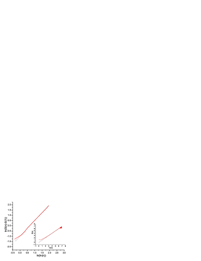
Figure 4: The time evolution of the coarse-grained entropy for the triangle map, computed by taking $5\times 10^{7}$ points initially distributed randomly in one cell of a $N\times N$ phase-space grid with $N=700$. We plot $\ln(S(n)-S(1))$ versus $\ln\ln n$. The straight line has slope $3/2$. Obviously, the entropy will eventually saturate at $S(\infty)=\ln N^{2}$. In the inset we show the entropy computed for the uniquely-ergodic and nonmixing dynamics with $\alpha=0$. The dotted line has slope $1$.

Finally we would like to stress that this behavior of the triangle map differs from the typical behavior which has been found for chaotic or for integrable systems. In particular, contrary to the case of exponentially unstable systems, in this case the rate of fidelity decay depends on the perturbation strength. This feature is shared by quantum systems in which exponential instability is absent as well. One may wonder if this behavior is reflected also in some other, perhaps even more fundamental dynamical property of the map. In order to explore this question, we have computed the entropy production for the map (1). As the extensive computation of Kolmogorov-Sinai dynamical entropies seemed too expensive for reaching any conclusive results, we have decided to compute the dynamical evolution of the coarse grained statistical entropy $S_{n}=-\sum_{j}p_{n}^{(j)}\ln p_{n}^{(j)}$. To this end we divide the phase space in $N\times N$ equal cells, and consider an initial ensemble of points uniformly distributed over one cell. The probability $p_{n}^{(j)}$ is defined as the fraction of orbits which, after $n$ time steps, fall in the cell of label $j$. For a chaotic system with dynamical entropy $h$, one expects $S_{n}=hn+{\rm const}$ latora , whereas for ergodic-only (non-mixing) dynamics one expects $S_{n}\sim\ln n$, for sufficiently large $N$. Our numerical results for the triangle map (fig. 4) show instead that $S_{n}-S_{1}=|\ln n|^{\lambda}$ with the exponent $\lambda=3/2$. Furthermore, as shown in the inset of fig.4, for the triangle map (1) with $\alpha=0$ numerical results give, quite accurately, $S(n)=\ln n$ (with no prefactor or additional constant).

In conclusion, we have discussed the parametric stability, as characterized by classical fidelity or Loschmidt echo, of an important class of dynamical systems where neutral stability is coexisting with dynamical mixing. As a paradigmatic example of this class of systems we have considered the triangle map. By means of analytic calculations and numerical simulations we have derived two universal regimes of fidelity decay, both being characterized by a universal scaled time variable $|\delta|^{2/5}t$. This interesting dynamical behavior is supported also by a power-logarithmic behavior of the coarse-grained entropy.

We acknowledge financial support by the PRIN 2002 “Fault tolerance, control and stability of quantum information processing” and PA INFM “Weak chaos: Theory and applications” (GC), by the grant P1-044 of Ministry of Education, Science and Sport of Slovenia (TP), by the grant DAAD19-02-1-0086, ARO United States (GC and TP), and by the Faculty Research Grant of NUS and the Temasek Young Investigator Award of DSTA, Singapore under project agreement POD0410553 (BL).

References

- (1) A. Peres, Phys. Rev. A 30, 1610 (1984).
- (2) H. M. Pastawski et al., Physica A 283, 166 (2000).
- (3) R. A. Jalabert and H. M. Pastawski, Phys. Rev. Lett. 86, 2490 (2001).
- (4) T. Prosen, Phys. Rev. E 65, 036208 (2002).
- (5) Ph. Jacquod et al. Phys. Rev. E 64, 055203(R) (2001).
- (6) N. R. Cerruti and S. Tomsovic, Phys. Rev. Lett. 88, 054103 (2002).
- (7) G. Benenti and G. Casati, Phys. Rev. E 65, 066205 (2002).
- (8) T. Prosen and M. Žnidarič, J. Phys. A 35, 1455 (2002).
- (9) B. Eckhardt, J. Phys. A: Math. Gen 36, 371 (2003).
- (10) G. Benenti, G. Casati and G. Veble, Phys. Rev. E 67, 055202 (2003).
- (11) G. Veble, T. Prosen, Phys. Rev. Lett. 92, 034101 (2004).
- (12) G. Benenti, G. Casati and G. Strini, Principles of Quantum Computation and Information, Vol. I: Basic Concepts (World Scientific, Singapore, 2004); M. A. Nielsen and I. L. Chuang, Quantum computation and quantum information (Cambridge UP, 2001).
- (13) G. Casati, T. Prosen, Phys. Rev. Lett. 83, 4729 (1999).
- (14) G. Casati, T. Prosen, Phys. Rev. Lett. 85, 4261 (2000)
- (15) Strictly speaking there is no rigorous proof that irrational polygons are mixing. We refer here to the evidence provided by numerical computations such as those reported in refs. caspro99 ; caspro00 .
- (16) M. Degli Esposti and S. Galatolo, preprint http://www.dm.unibo.it/fismat/pub/CPco010404.pdf
- (17) V. Latora, M. Baranger, Phys. Rev. Lett. 82, 520 (1999).