Stability and collisions of moving semi-gap solitons in Bragg cross-gratings

Abstract

We report results of a systematic study of one-dimensional four-wave moving solitons in a recently proposed model of the Bragg cross-grating in planar optical waveguides with the Kerr nonlinearity; the same model applies to a fiber Bragg grating (BG) carrying two polarizations of light. We concentrate on the case when the system’s spectrum contains no true bandgap, but only semi-gaps (which are gaps only with respect to one branch of the dispersion relation), that nevertheless support soliton families. Solely zero-velocity solitons were previously studied in this system, while current experiments cannot generate solitons with the velocity smaller than half the maximum group velocity. We find the semi-gaps for the moving solitons in an analytical form, and demonstrated that they are completely filled with (numerically found) solitons. Stability of the moving solitons is identified in direct simulations. The stability region strongly depends on the frustration parameter, which controls the difference of the present system from the usual model for the single BG. A completely new situation is possible, when the velocity interval for stable solitons is limited not only from above, but also from below. Collisions between stable solitons may be both elastic and strongly inelastic. Close to their instability border, the solitons collide elastically only if their velocities $c_{1}$ and $c_{2}$ are small; however, collisions between more robust solitons are elastic in a strip around $c_{1}=-c_{2}$.

1 Introduction

Bragg gratings (BGs) are broadly used as a basis for spectral filters are other elements of optical telecommunication networks [1]. Simultaneously, BGs offer a unique medium for the theoretical [2] – [14] and experimental [15] study of gap solitons (GSs), supported by the balance between the BG-induced dispersion and Kerr (cubic) nonlinearity dispersion . The latter topic was surveyed in an earlier review [16] and recent one [17]. Matter-wave pulses similar to the optical BG solitons were very recently observed in Bose-Einstein condensates [18].

The BG solitons may exist not only as temporal pulses in fiber gratings, but also as spatial solitons in 2D (two-dimensional) waveguides [19]. In the latter case, the BG is represented by a set of parallel grooves on the surface of the waveguide. A generalization, that makes it possible to increase the number of waves coupled by the BG, is based on a superposition of more than one BGs in the spatial domain. In particular, a system of three gratings which form a triangular lattice was considered in Ref. [12]. It couples three waves, giving rise to new types of stable GSs – for instance, “peakons”.

In recent papers [20] and [21], a model of a cross-grating was introduced, as a superposition of two mutually transverse BGs written on a 2D waveguide with the Kerr nonlinearity. In this case, one is dealing with a system of four waves. The evolution of their amplitudes $v_{j}$, $j=1,2,3,4$, obeys the system of normalized equations [20, 21],

$${\small i}\frac{\partial v_{1}}{\partial t}+\frac{i}{\sqrt{2}}\frac{\partial v_{1}}{\partial z}+\frac{i}{\sqrt{2}}\frac{\partial v_{1}}{\partial x}+v_{2}+\mu v_{3}+\left[\left|v_{1}\right|^{2}+2(\left|v_{2}\right|^{2}+\left|v_{3}\right|^{2}+\left|v_{4}\right|^{2})\right]v_{1}+2v_{2}v_{3}v_{4}^{\ast} = {\small 0,}$$

$$i\frac{\partial v_{2}}{\partial t}-\frac{i}{\sqrt{2}}\frac{\partial v_{2}}{\partial z}+\frac{i}{\sqrt{2}}\frac{\partial v_{2}}{\partial x}+v_{1}+\mu v_{4}+\left[\left|v_{2}\right|^{2}+2(\left|v_{1}\right|^{2}+\left|v_{3}\right|^{2}+\left|v_{4}\right|^{2})\right]v_{2}+2v_{1}v_{4}v_{3}^{\ast} = 0,$$

$$i\frac{\partial v_{3}}{\partial t}+\frac{i}{\sqrt{2}}\frac{\partial v_{3}}{\partial z}-\frac{i}{\sqrt{2}}\frac{\partial v_{3}}{\partial x}+v_{4}+\mu v_{1}+\left[\left|v_{3}\right|^{2}+2(\left|v_{1}\right|^{2}+\left|v_{2}\right|^{2}+\left|v_{4}\right|^{2})\right]v_{3}+2v_{1}v_{4}v_{2}^{\ast} = 0,$$

$$i\frac{\partial v_{4}}{\partial t}-\frac{i}{\sqrt{2}}\frac{\partial v_{4}}{\partial z}-\frac{i}{\sqrt{2}}\frac{\partial v_{4}}{\partial x}+v_{3}+\mu v_{2}+\left[\left|v_{4}\right|^{2}+2(\left|v_{1}\right|^{2}+\left|v_{3}\right|^{2}+\left|v_{2}\right|^{2})\right]v_{4}+2v_{2}v_{3}v_{1}^{\ast} = 0.$$ (1)

Here, $t$ is time, $x$ and $z$ are the coordinates in the waveguide, the Bragg reflectivity (strength) of one grating is normalized to be $1$, and $\mu$ is a relative strength of the second grating. Coefficients in front of the nonlinear terms in Eqs. (1), which represent the self-phase-modulation, cross-phase-modulation and four-wave-mixing, correspond to the normal Kerr effect in isotropic materials.

The same model finds a different interpretation in terms of a 3D photonic crystal with a transverse chess-board structure [20, 21]. In that case, Eqs. (1), with $t$ replaced by the third coordinate $y$, along which the medium is homogeneous, govern the spatial evolution of the time-independent fields. In the latter context, a model which is tantamount to the particular symmetric case of the system (1), with $\mu=1$, was earlier introduced in Ref. [22] (in fact, this case is a degenerate one, as it corresponds to the gap in the model’s linear spectrum collapsing to a point [20, 21]). Ref. [22] was dealing with 2D solitons, treating their stability by means of a method which is tantamount to the known Vakhitov-Kolokolov (VK) criterion [23]. In fact, this method is not sufficient for the verification of the stability, and our direct simulations (to be reported elsewhere) demonstrate that all the 2D solitons, both in the general system (1) and in its special case with $\mu=1$ that was considered in Ref. [22], are unstable.

A simpler possibility is to consider 1D solitons, which are generated by the substitution $v_{j}(t,x,z)\equiv e^{ikz}u_{j}(t,x)$ in Eqs. (1),

$$i\frac{\partial u_{1}}{\partial t}-\frac{k}{\sqrt{2}}u_{1}+\frac{i}{\sqrt{2}}\frac{\partial u_{1}}{\partial x}+u_{2}+\mu u_{3}+\left[\left|u_{1}^{2}\right|+2(\left|u_{2}^{2}\right|+\left|u_{3}^{2}\right|+\left|u_{4}^{2}\right|)\right]u_{1}+2u_{2}u_{3}u_{4}^{\ast} = 0,$$

$$i\frac{\partial u_{2}}{\partial t}+\frac{k}{\sqrt{2}}u_{2}+\frac{i}{\sqrt{2}}\frac{\partial u_{2}}{\partial x}+u_{1}+\mu u_{4}+\left[\left|u_{2}^{2}\right|+2(\left|u_{1}^{2}\right|+\left|u_{3}^{2}\right|+\left|u_{4}^{2}\right|)\right]u_{2}+2u_{1}u_{4}u_{3}^{\ast} = 0,$$

$$i\frac{\partial u_{3}}{\partial t}-\frac{k}{\sqrt{2}}u_{3}-\frac{i}{\sqrt{2}}\frac{\partial u_{3}}{\partial x}+u_{4}+\mu u_{1}+\left[\left|u_{3}^{2}\right|+2(\left|u_{1}^{2}\right|+\left|u_{2}^{2}\right|+\left|u_{4}^{2}\right|)\right]u_{3}+2u_{1}u_{4}u_{2}^{\ast} = 0,$$

$$i\frac{\partial u_{4}}{\partial t}+\frac{k}{\sqrt{2}}u_{4}-\frac{i}{\sqrt{2}}\frac{\partial u_{4}}{\partial x}+u_{3}+\mu u_{2}+\left[\left|u_{4}^{2}\right|+2(\left|u_{1}^{2}\right|+\left|u_{3}^{2}\right|+\left|u_{2}^{2}\right|)\right]u_{4}+2u_{2}u_{3}u_{1}^{\ast} = 0.$$ (2)

Note that Eqs. (2) conserve the Hamiltonian, momentum, and the norm (which is frequently called energy, in the applications to optics),

$$E=\sum_{j=1}^{4}\int_{-\infty}^{+\infty}\left|u_{j}(x)\right|^{2}dx.$$ (3)

The model based on Eqs. (2) is of special interest, as previously considered multi-wave GS models, such as the three-wave one in Ref. [24], did not contain a parameter similar to $k$, which accounts for frustration, i.e., symmetry breaking in the wave pairs $\left(u_{1},u_{2}\right)$ and $\left(u_{3},u_{4}\right)$ in Eqs. (2). In fact, the frustration makes the present four-wave distinct from the usual two-wave BG model.

The same system (2) also finds an interpretation in terms of the BG in optical fibers. In that case, the fields $u_{1,2}$ and $u_{3,4}$ in Eqs. (2) represent pairs of right- and left-travelling waves with two orthogonal circular polarizations, $\mu$ is the Bragg-reflectivity strength, while the linear-coupling terms with the coefficient $1$ account for linear mixing between the circular polarizations due to an elliptic deformation of the fiber’s core, and the terms proportional to $k$ take into regard birefringence due to a twist of the fiber.

Looking for solutions to the linearized version of Eqs. (2) as $u_{j}(x,t)\sim\exp\left(i\lambda x-i\omega t\right)$, one arrives at a dispersion relation,

$$\omega^{2}=\frac{1}{2}\left(\sqrt{2\mu^{2}+\lambda^{2}}\pm\sqrt{2+k^{2}}\right)^{2},$$ (4)

which generates a bandgap in the spectrum, $\left|\omega\right|<\omega_{\mathrm{edge}}\equiv\mu-\sqrt{1+\left(k^{2}/2\right)}$, provided that $\mu^{2}>1+\left(k^{2}/2\right)$. Besides the gap, the two branches of the dispersion relation (4) give rise to semi-gaps, $\max\left\{\mu-\sqrt{1+\left(k^{2}/2\right)},0\right\}<\left|\omega\right|<\mu+\sqrt{1+\left(k^{2}/2\right)}$, which are also found in the case of

$$\mu^{2}<1+\left(k^{2}/2\right),$$ (5)

when the full gap is absent. It was recently shown, in a general form, that families of BG solitons may exist in semi-gaps even if the full gap is absent [24].

Quiescent (zero-velocity) solitons in Eqs. (2), of the form $u_{j}(x,t)=U_{j}(x)\exp\left(-i\omega t\right)$, were investigated in detail in Ref. [20] [solitons generated by Eqs. (1) in the spatial domain, corresponding to $u_{j}(t,z,x)=\exp\left(-i\omega t\right)U_{j}(z,x)$ with fixed $\omega$, were studied in Ref. [21]]. They obey a reduction $U_{3}=-U_{1}^{\ast},\,U_{4}=-U_{2}^{\ast}$, which is not valid for moving solitons, see below. If $k=0$, the solitons fall into three categories: symmetric and anti-symmetric ones, with $U_{1}=\pm U_{2}$, and more general asymmetric solitons. The latter ones, and the solitons obtained by their continuation to $k\neq 0$, are always subject to a weak instability. The symmetric and anti-symmetric solitons, as well as those stemming from them at $k\neq 0$, were found, respectively, to be stable chiefly (but not exclusively) in the full gap (if any), and in the semi-gaps outside the full gap.

Moving solitons are to be looked for solitons in the form

$$u_{j}(x,t)=\exp\left(-i\omega t\right)U_{j}(\xi),~{}\xi\equiv x-ct.$$ (6)

Straightforward consideration of the underlying system (2) shows that moving solitons may exist for $|c|~{}<c_{\max}=1/\sqrt{2}$ [20] . On the other hand, quiescent BG solitons have never been observed in the experiment, the minimum velocity at which they could be created being, roughly, $c_{\max}/2$ [15] (a possibility to diminish the velocity through collisions between the moving solitons was proposed in Ref. [25]). In Ref. [20], moving solitons in the present model were considered, in a brief form, inside the full gap. It was found that they loose their stability at quite small values of the velocity, $\simeq 0.2c_{\max}$. Our aim is to study the stability of the moving solitons in a systematic way, as well as collisions between them. We will consider moving solitons in the most interesting case, when the full bandgap does not exist, but, nevertheless, solitons may be found in the semi-gaps (see above). To the best of our knowledge, the moving solitons in this case has never been considered before.

2 Existence and stability of the moving solitons

To look for solitons in the form (6), one can rewrite the underlying equations (2) in terms of the variables $(t,\xi)$. The linearization of the equations gives rise to a dispersion relation, which differs from (4) by the replacement $\omega\rightarrow\omega+c\lambda$. In the case when the spectrum contains no full gap, straightforward analysis yields an equation to for the values of $\omega$ at edges of the semi-gaps, where we aim to find the solitons:

$$\left[\omega\pm\sqrt{1+\left(k^{2}/2\right)}\right]^{2}=\mu^{2}\left(1-2c^{2}\right)~{}.$$ (7)

It immediately follows from Eq. (7) that no semi-gaps, hence no solitons either, are possible for $|c|~{}>1/\sqrt{2}$. Typical examples of the semi-gap in the plane $\left(c,\omega\right)$ are shown in Fig. 1.

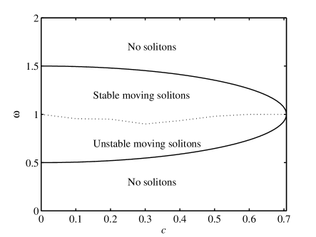
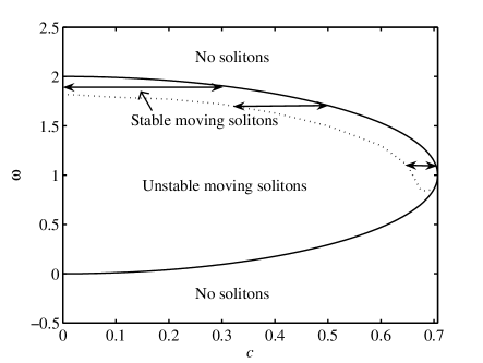
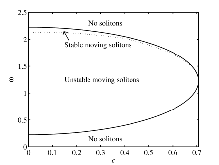
Fig. 1: The solid curves are edges of the semi-gap, determined in the analytical form by Eq. (7) with the lower sign in the left-hand side [a counterpart of this semi-gap, corresponding to the upper sign in Eq. (7), is located at $\omega<0$]. The region between the solid curves (the semi-gap proper) is completely filled by the solitons, the dotted curve being the border between stable and unstable ones, as identified in direct simulations. Shown are typical examples for the cases of zero frustration, $k=0$,$\mu=0.5$ (a), small frustration, $k=0.005$,$\mu=1$ (b), and large frustration, $k=1$,$\mu=1$ (c). Three double arrow lines in (b) are cross sections of the stability region for $\omega=\mathrm{const}$, which correspond to Eqs. (8).

Stationary equations, which are obtained by the substitution of Eq. (6) into Eqs. (2), were solved by means of the shooting method. The numerical solution shows that the semi-gaps are, indeed, completely filled by solitons. Note that the moving solitons cannot be generated automatically from quiescent ones, as Eqs. (2) bear no Galilean or Lorentzian invariance.

Stability of the solitons was identified in direct simulations of Eqs. (2) for perturbed solutions, by means of the split-step Fourier-transform and finite-difference techniques, both methods yielding identical results. Typical examples of the stable moving solitons, found inside the semi-gaps, are displayed in Fig. 2.

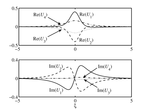
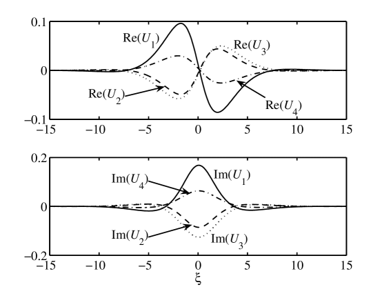
Fig. 2: Generic examples of stable moving solitons in the form of Eq. (6), found by the shooting method. Shown are real and imaginary parts of the four fields. The panel (a) and (b) represent, respectively, the cases of zero ($k=0,\mu=0.5,c=0.5,\omega=1$) and finite ($k=1,\mu=1,c=0.2,\omega=2.13$) frustration.

As well as in the case of zero-velocity solitons [20], the frustration parameter $k$ strongly affects the solitons’ shape and stability: if $k=0$, the stability area is largest, and the stable solitons obey the reduction $U_{1,3}=-U_{2,4}$. As is seen in Figs. 2 and 1, nonzero frustration breaks the latter relations, and leads to strong shrinkage of the stability region.

A notable feature is that, in the case of small but finite $k$, the stability interval for a fixed value of $\omega$ may be limited not only by a maximum value of the soliton’s velocity, but also by a minimum one. For example, three cross sections shown by arrows in Fig. 1(b) (for $k=0.005$ and $\mu=1$) correspond to the stability intervals

$$0 \leq |c|<0.3082~{}\mathrm{for}~{}\omega=1.9;~{}$$

$$0.28 < |c|<0.5049~{}\mathrm{for}~{}\omega=1.7,~{}0.6595<|c|<0.70356~{}\mathrm{for}~{}\omega=1.1,$$ (8)

the two latter ones being limited by a minimum value of $c$. The fact that the stability of the solitons may require a finite velocity is a completely new one. Nothing similar occurs in the model supporting the usual two-wave GSs [4].

The stability of solitons is not sensitive to the value of the relative Bragg reflectivity $\mu$, unlike the frustration $k$. In particular, the variation of $\mu$ does not essentially change the shape of the stability region displayed in Fig. 1, nor the shape of the solitons shown in Fig. 2.

Note that stability of the solitons against non-oscillatory perturbations (those corresponding to real stability eigenvalues) is provided, at fixed $c$, by the above-mentioned VK criterion, $dE/d\omega<0$ [23] [recall the soliton’s energy $E$ is defined as per Eq. (3)]. The applicability of the VK criterion to the present model was not rigorously proven, but in Ref. [22] it was actually derived for the particular case of $\mu=1$. Inspection of numerical data shows that all the solitons satisfy this criterion; however, it does not preclude instability against oscillatory perturbations (those corresponding to pairs or quartets of complex instability eigenvalues), that is why a part of the solitons are unstable. Further simulations demonstrate that the development of the instability always leads to complete destruction of the soliton, see a typical example in Fig. 3.

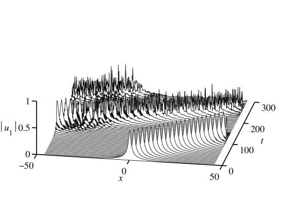
Fig. 3: A typical example of the destruction of an unstable soliton, observed in direct simulations of Eqs. (2). Here (as well as in Figs. 4 and 5 below) shown is the evolution of the field $\left|u_{1}\right|$; in other components, the evolution is quite similar. The parameters are $k=0,\mu=0.5,c=0.4,\omega=0.6$. The figure uses the original coordinate $x$, rather than $\xi$ from Eq. (6).

3 Collisions between moving solitons

The next step in the study of the moving solitons is to consider collisions between them, which is interesting in its own right, and for various applications too [25]. As Eqs. (2) are not integrable, an issue is whether collisions between stable solitons will be elastic or not. We stress that neither the stability of the solitons of the semi-gap type, considered in this paper, nor collisions between them were considered in earlier works.

Exploring the stability region of the moving solitons (see Fig. 1), we have found that collisions between them may be both completely elastic, leading to no other effect but finite shifts of the colliding solitons, and strongly inelastic, resulting in a partial destruction of the solitons, and generation of large amounts of radiation. Typical examples of these outcomes are shown in Figs. 4 and 5. The interaction between the elastically colliding solitons has the character of the bounce from each other.

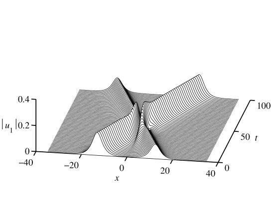
Fig. 4: A typical example of the elastic collision between two identical stable solitons moving with the velocities $c_{1,2}=\pm 0.3$, the other parameters being $k=1,\mu=1,\omega=2.08$.

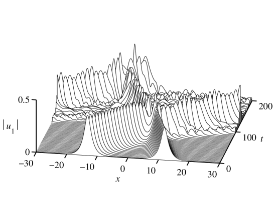
Fig. 5: A typical example of the inelastic collision between two stable solitons moving with the velocities $c_{1}=-0.1$ and $c_{2}=+0.25$. The other parameters are $k=0,\mu=0.5,\omega=1$.

The outcome of the collision strongly depends on the solitons’ velocities $c_{1,2}$. Therefore, the results can be naturally summarized in the form of a region in the plane $\left(c_{1},c_{2}\right)$ where the collisions are elastic; at the border of the region, the transition between the two types of the collision is found to be quite sharp. In turn, the size of the region of the nondestructive (elastic) collisions depends on proximity of the individual solitons to the instability border in their parameter planes, see Fig. 1.

First, in Fig. 6 we present these results for the zero-frustration case ($k=0$), when the stability region in Fig. 1(a) is quite large. As it follows from the inspection of Fig. 1(a), the difference between the three cases displayed in Fig. 6 is that in the case of $\omega=1$ (a) the colliding solitons are close to the instability border, while in the other cases, $\omega=1.2$ (b) and $\omega=1.4$ (c), they are located deeper in the stability region (in the latter case, the soliton is actually close to the edge of the semi-gap, i.e., the existence border of the solitons). Accordingly, there is a notable difference in the shape of the elasticity region in the $\left(c_{1},c_{2}\right)$ plane: in the first case, the collisions may be elastic only if the velocities are small, while in the other cases, the solitons with large but nearly opposite velocities, $c_{1}\approx-c_{2}$, collide elastically even if the velocities are large.

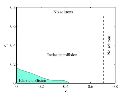
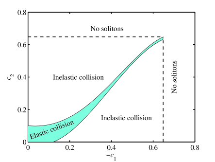
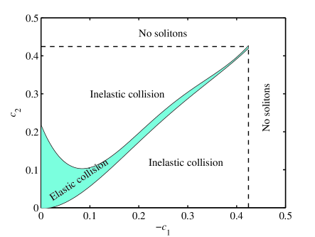
Fig. 6: Areas of elastic and inelastic collisions between solitons in the plane of their velocities, $\left(c_{1},c_{2}\right)$ (the values up to the limiting value, $c_{\max}=1/\sqrt{2}\approx\allowbreak 0.71$, are shown). The fixed parameters are $k=0$ and $\mu=0.5$. The frequency is $\omega=1.0$ (a), $1.2$ (b), $1.4$ (c). The horizontal and vertical dashed lines limit the velocity intervals of the stable solitons, as per Fig. 1.

As it was stressed above, in the case of finite frustration, the velocity interval corresponding to the stable solitons may be limited not only from above, but also from below. The collisions between unstable solitons being definitely destructive, the latter fact strongly affects the region of elastic (nondestructive) collisions in the $\left(c_{1},c_{2}\right)$ plane for $k\neq 0$, as is seen in Fig. (7).

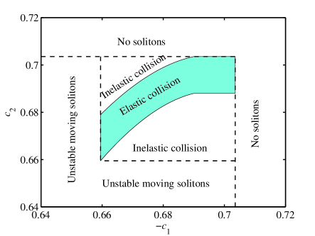
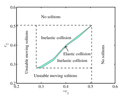
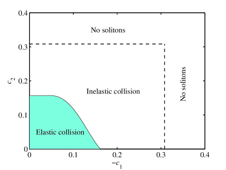
Fig. 7: The same as in Fig. (6) for the case of nonzero frustration, $k=0.005$ and $\mu=1$. The fixed frequency is $\omega=1.1$ (a), $1.7$ (b), $1.9$ (c).

As it was mentioned above, in the currently feasible experiments with BG solitons, their velocity cannot be made smaller than, approximately, half the maximum group velocity, which is $1/\sqrt{2}$ in the present notation. For this reason, it is quite important that the elasticity regions shown in Figs. 6(b,c) and 7(a,b) extend to large values of $c$.

Lastly, it is necessary to mention that, as well as the stability of individual solitons, the outcome of the collisions is not sensitive to the relative BG reflectivity $\mu$, on the contrary to the strong dependence on the frustration $k$. In fact, the elasticity regions show almost no dependence on $\mu$, therefore the examples shown in Figs. 6 and 7 are quite generic ones.

4 Conclusion

In this paper, we have presented results of a systematic study of the stability and collisions of moving four-wave solitons in the recently introduced model of the Bragg cross-grating in planar optical waveguides with the Kerr nonlinearity. We have focused on the case when the system’s linear spectrum does not contain any true bandgap, but rather features semi-gaps, in which soliton families may be found. In recent works, only zero-velocity solitons in this four-wave system have been studied. That case is far from the current experiments, which generate solitons whose velocity exceed, roughly, half the maximum group velocity. We have found the semi-gaps for the moving solitons in the analytical form, and demonstrated that numerically found solitons completely fill the semi-gaps. Stability of the moving solitons was determined by direct simulations, revealing a stability border which strongly depends on the frustration parameter. It is interesting that a previously unknown situation is possible in the present model, when the velocity interval for stable solitons is limited not only from above, but also from below.

Collisions between stable solitons may be both elastic, so that they bounce from each other, and strongly inelastic, leading to a partial destruction of the solitons, with a sharp border between the two outcomes. A region of elastic collisions was identified, with a well-pronounced peculiarity: if the individual solitons are close to the stability border, they collide elastically only if their velocities $c_{1}$ and $c_{2}$ are small; however, if the solitons are more stable, the collision remains elastic in a strip around the line $c_{1}=-c_{2}$. As well as the stability of individual solitons, the elasticity region strongly depends on the frustration parameter, but is insensitive to the relative reflectivity of the two Bragg gratings which constitute the cross configuration.

References

- [1] R. Kashyap, Fiber Bragg gratings (Academic Press: San Diego, 1999).
- [2] A.B. Aceves and S. Wabnitz, Phys. Lett. A 141, 37 (1989); D. N. Christodoulides and R.I. Joseph, Phys. Rev. Lett. 62, 1746 (1989).
- [3] B.A. Malomed and R. S. Tasgal, Phys. Rev. E 49, 5787 (1994)
- [4] I. V. Barashenkov, D. E. Pelinovsky, and E. V. Zemlyanaya, Phys. Rev. Lett. 80, 5117 (1998).
- [5] A. De Rossi, C. Conti, and S. Trillo, Phys. Rev. Lett. 81, 85 (1998).
- [6] J. Schollmann and A. P. Mayer, Phys. Rev. E 61, 5830 (2000).
- [7] W. Mak, B.A. Malomed, and P. L. Chu, J. Opt. Soc. Am. B 15, 1685 (1998).
- [8] A. R. Champneys, B. A. Malomed, and M. J. Friedman, Phys. Rev. Lett. 80, 4169 (1998).
- [9] E. N. Tsoy and C. M. de Sterke, J. Opt. Soc. AM. B 18, 1 (2001).
- [10] J. Atai, B.A. Malomed, Phys. Rev. E 62, 8713 (2000), ibid. E 64, 066617 (2001); Phys. Lett. A 298, 140 (2002).
- [11] G. Curatu, S. LaRochelle, C. Paré, and P. A. Belanger, Electron. Lett. 38, 307 (2002).
- [12] R. Grimshaw, B.A. Malomed, and G. A. Gottwald, Phys. Rev. E 65, 066606 (2002).
- [13] H. Y. Tseng and S. Chi, Phys. Rev. E 66, 056606 (2002).
- [14] R. H. Goodman, R. E. Slusher, and M. I. Weinstein, J. Opt. Soc. Am. B 19, 1635 (2002); W. C. K. Mak, B. A. Malomed, and P. L. Chu, ibid. 20, 725 (2003); Phys. Rev. E 67, 026608 (2003).
- [15] B. J. Eggleton, R. E. Slusher, C. M. de Sterke, P. A. Krug, and J. E. Sipe, Phys. Rev. Lett. 76, 1627 (1996); C. M. de Sterke, B. J. Eggleton, and P. A. Krug, J. Lightwave Technol. 15, 1494 (1997); B. J. Eggleton, C. M. de Sterke, and R. E. Slusher, J. Opt. Soc. Am. B 16, 587 (1999).
- [16] C. M. de Sterke and J. E. Sipe, Progr. Opt. 33, 203 (1994).
- [17] C. Conti, G. Assanto, and S. Trillo, J. Nonlin. Opt. Phys. Mat. 11, 239 (2002).
- [18] R. G. Scott, A. M. Martin, T. M. Fromhold, S. Bujkiewicz, F. W. Sheard, and M. Leadbeater, Phys. Rev. Lett. 90, 110404 (2003); B. Eiermann, T. Anker, M. Albiez, M. Taglieber, P. Treutlein, K. P. Marzlin, and M. K. Oberthaler, Phys. Rev. Lett. 92, 230401 (2004).
- [19] J. Feng, Opt. Lett. 18, 1302 (1993).
- [20] I. M. Merhasin and B. A. Malomed, J. Optics B: Quant. Semiclass. Opt. 6, S323 (2004).
- [21] I. M. Merhasin and B. A. Malomed, Phys. Lett. A 327, 296 (2004).
- [22] N. Aközbek and S. John, Phys. Rev. E 57, 2287 (1998).
- [23] M.G. Vakhitov and A.A. Kolokolov, Radiophys. Quantum Electr. 16, 783 (1973); see also a review by L. Bergé, Phys. Rep. 303, 260 (1998).
- [24] W. C. K. Mak, B. A. Malomed, and P. L. Chu, Phys. Rev. E 69, 066610 (2004).
- [25] W. C. K. Mak, B. A. Malomed, and P. L. Chu, Phys. Rev. E 68, 026609 (2003).