An unusual Liénard type nonlinear oscillator with properties of a linear harmonic oscillator

Abstract

A Liénard type nonlinear oscillator of the form $\ddot{x}+kx\dot{x}+\frac{k^{2}}{9}x^{3}+\lambda_{1}x=0$, which may also be considered as a generalized Emden type equation, is shown to possess unusual nonlinear dynamical properties. It is shown to admit explicit nonisolated periodic orbits of conservative Hamiltonian type for $\lambda_{1}>0$. These periodic orbits exhibit the unexpected property that the frequency of oscillations is completely independent of amplitude and continues to remain as that of the linear harmonic oscillator. This is completely contrary to the standard characteristic property of nonlinear oscillators. Interestingly, the system though appears deceptively a dissipative type for $\lambda_{1}\leq 0$ does admit a conserved Hamiltonian description, where the characteristic decay time is also independent of the amplitude. The results also show that the criterion for conservative Hamiltonian system in terms of divergence of flow function needs to be generalized.

I Introduction

Nonlinear oscillator systems are ubiquitous and they model numerous physical phenomena ranging from atmospheric physics, condensed matter, nonlinear optics to electronics, plasma physics, biophysics, evolutionary biology, etc. Nay:1989 ; Guc:1983 ; Tab:1989 ; Wig:2003 ; Lak:2003 . One of the most important characteristics of nonlinear oscillations is the amplitude or initial condition dependence of frequency for nonisolated periodic orbits Nay:1989 ; Tab:1989 ; Lak:2003 . For example, for the cubic anharmonic oscillator

$$\ddot{x}+\omega_{0}^{2}x+\beta x^{3}=0,\qquad(\omega_{0}^{2},\beta>0),$$ (1)

where dot denotes differentiation with respect to $t$, the general (periodic) solution is $x(t)=A\;cn(\Omega t+\delta)$, where $A$ and $\delta$ are arbitrary constants with the modulus squared of the Jacobian elliptic function $m^{2}=\frac{\beta A^{2}}{2(\omega_{0}^{2}+\beta A^{2})}$ and frequency $\Omega=\sqrt{\omega_{0}^{2}+\beta A^{2}}$. In the case of limit cycle oscillations the dependence of the initial condition is manifested in the form of suitable transient time to reach the asymptotic state. For chaotic oscillations, of course, there is the sensitive dependence on initial conditions. In this paper we identify a physically interesting and simple nonlinear oscillator of the Liénard type, which is also a generalized Emden type equation, that admits for a particular sign of the control parameter nonisolated conservative periodic oscillations, exhibiting the remarkable fact that the frequency of oscillation is completely independent of amplitude and remains the same as that of the linear harmonic oscillator, thereby showing that the amplitude dependence of frequency is not necessarily a fundamental property of nonlinear dynamical phenomena. We also show that rewriting the underlying equation of motion as a system of two first order coupled nonlinear differential equations the basic criterion for conservative system in terms of the divergence of the flow function has to be generalized.

We consider a nonlinear oscillator system of the form

$$\ddot{x}+kx\dot{x}+\frac{{k}^{2}}{9}x^{3}+\lambda_{1}x=0,$$ (2)

which is of the Liénard type $\ddot{x}+f(x)\dot{x}+g(x)=0$, where $f(x)=kx$ and $g(x)=\frac{{k}^{2}}{9}x^{3}+\lambda_{1}x$ in the present case. Eq. (2) can also be interpreted as the cubic anharmonic oscillator defined by Eq. (1) (with $\omega_{0}^{2}=\lambda_{1}$ and $\beta=\frac{k^{2}}{9}$), but acted upon on by a strong damping type nonlinear force $kx\dot{x}$. This type of equation is also well studied in the literature for almost two decades as a generalized form of Emden type equation occurring in the study of equilibrium configurations of a spherical cloud acting under the mutual attraction of its molecules and subject to the laws of thermodynamics Dix:1990 . Eq. (2) is a special case of a general second order nonlinear differential equation possessing eight Lie point symmetries mah:1985 and that it is linearizable. In particular the special case $\lambda_{1}=0$ has been well analyzed by Mahomed and Leach mah:1985 and explicit forms of the eight symmetry generators satisfying $sl(3,R)$ algebra have been well documented. The latter case $(\lambda_{1}=0)$ has the exact general solution

$$x(t)=\frac{t+I_{1}}{\frac{k}{6}t^{2}+\frac{I_{1}k}{3}t+I_{2}},$$ (3)

where $I_{1}$ and $I_{2}$ are the two integrals of motion with the explicit forms

$$I_{1}=-t+\frac{x}{\frac{k}{3}x^{2}+\dot{x}},\;\;$$ (4a)

$$I_{2}=\frac{k}{6}t^{2}+\frac{1-\frac{k}{3}tx}{\frac{k}{3}x^{2}+\dot{x}}.$$ (4b)

Obviously for $\lambda_{1}=0$ case the initial value problem of Eq. (2) appears to be a dissipative nonlinear system.

In the following we show that the nonlinear oscillator equation (2) possesses several unusual and interesting features, which are contrary to the standard characteristic features associated with usual nonlinear oscillators. For example, in the case $\lambda_{1}>0$ we prove that the system (2) possesses oscillatory motion whose frequency is completely independent of the amplitude. Thus we prove that the standard notion of amplitude dependent frequency of oscillations is not a necessary condition for nonlinear oscillators. Moreover, we also point out that the system (2) admits a Lagrangian formulation and from which a conservative Hamiltonian can be obtained. Further, we also find that the standard test (divergence of the flow function) to identify whether the given system is conservative or not fails here. To overcome this situation we propose that the necessary condition for a system to be a conserved Hamiltonian is that the time average of the divergence of the flow function should vanish instead of the flow function itself vanishing. More interestingly, we also find that the system (2) when $\lambda_{1}\leq 0$ also admits a Lagrangian as well as a conserved Hamiltonian description similar to the case $\lambda_{1}>0$, eventhough the general solution shows a dissipative/damping/frontlike aperiodic structure, depending on the initial condition. The divergence of the flow function for the case $\lambda_{1}\leq 0$ can be negative for all times in spite the conserved Hamiltonian nature. Again to redeem the situation, one requires the time average of the divergence of the flow function to be vanishing. Finally, we also point out that the special features of the system can be traced to the existence of certain linearizing and canonical and nonlocal transformations, which points out to generalization of the results in different directions.

The plan of the paper is as follows. In the following section, we utilize the so called modified Prelle-Singer procedure and derive two functionally independent integrals of motion for the Eq. (2). In Sec. III, we show that for the case $\lambda_{1}>0$ the system (2) admits periodic solutions and construct the associated Lagrangian as well as Hamiltonian for this system. We discuss the unusual features associated with the system in Sec. IV and point out the amplitude independence of the frequency of oscillations as well as the nonzero value of the divergence of the flow function in spite of its conservative nature. We analyse the nature of solutions in the regimes $\lambda_{1}=0$ and $\lambda_{1}<0$ in Sec. V and point out that in spite of the decaying/damping nature or frontlike aperiodic nature of the solutions, the system admits Lagrangian and Hamiltonian descriptions. In Sec. VI, we linearize the Eq. (2) through different kinds of transformations (invertible point, nonlocal and canonical transformation) to trace the unusual features of the system. In Sec. VII, we generalize Eq. (2) and compare the dynamics with certain other interesting nonlinear oscillators. Finally, we present our conclusions in Sec. VIII.

II Extended Prelle-Singer procedure

Now let us consider the general case $\lambda_{1}\neq 0$. One can proceed to solve the equation explicitly by the so called modified Prelle-Singer (P-S) method Dua:2001 ; Cha:2004 which identifies the integrals of motion and explicit solution, if they exist. One can also use other methods as well; however we find that the P-S method is quite convenient Cha:2004 to obtain both the integrals of motion and solution explicitly. Assuming the existence of an integral $I=I(t,x,\dot{x})$ for Eq. (2) and rewriting the latter as $\ddot{x}=P(x,\dot{x})$, where $P=-kx\dot{x}-\frac{{k}^{2}}{9}x^{3}-\lambda_{1}x$, so that $Pdt-d\dot{x}=0$, and introducing a null term $S(t,x,\dot{x})\dot{x}dt-S(t,x,\dot{x})dx$, we find that on the solutions, $(P+S\dot{x})dt-Sdx-d\dot{x}=0$. Since $I$ is a constant of motion, it follows that

$$dI={I_{t}}{dt}+{I_{x}}{dx}+{I_{\dot{x}}{d\dot{x}}}=0,$$ (5)

so that

$$dI=R(P+S\dot{x})dt-RSdx-Rd\dot{x}=0,$$ (6)

where $R$ is an integrating factor. Comparing equations (5) with (6) we have, on the solutions, the relations

$$I_{t}=R(P+\dot{x}S)$$

$$I_{x}=-RS\qquad\;\;$$

$$I_{\dot{x}}=-R.\quad\qquad$$

Then the compatibility conditions, $I_{tx}=I_{xt}$, $I_{t\dot{x}}=I_{{\dot{x}}t}$, $I_{x{\dot{x}}}=I_{{\dot{x}}x}$, require that

$$D[S]=-P_{x}+SP_{\dot{x}}+S^{2},$$

$$D[R]=-R(S+P_{\dot{x}}),\qquad$$

$$R_{x}=R_{\dot{x}}S+RS_{\dot{x}},\qquad\;\;$$ (7)

where

$$D=\frac{\partial}{\partial{t}}+\dot{x}\frac{\partial}{\partial{x}}+P\frac{\partial}{\partial{\dot{x}}}.$$

Solving (7) systematically for $S$ and $R$, one can write down the form of the integral of motion,

$$I=r_{1}-r_{2}-\int\left[R+\frac{d}{d\dot{x}}\left(r_{1}-r_{2}\right)\right]d\dot{x},$$ (8)

where

$$r_{1}=\int R(P+\dot{x}S)dt,\quad r_{2}=\int(RS+\frac{d}{dx}r_{1})dx,$$

for the given form $P=-kx\dot{x}-\frac{{k}^{2}}{9}x^{3}-\lambda_{1}x$. We find two independent sets of compatible solutions of Eq. (7), namely,

$$S_{1}=\frac{-\dot{x}+\frac{k}{3}x^{2}}{x},\quad R_{1}=\frac{xe^{-2\sqrt{-\lambda_{1}}t}}{(\dot{x}+\frac{k}{3}x^{2}-\sqrt{\lambda_{1}}x)^{2}},$$ (9a)

$$S_{2}=\frac{(\frac{k}{3}x+\sqrt{-\lambda_{1}})^{2}-\frac{k}{3}\dot{x}}{\frac{k}{3}x+\sqrt{-\lambda_{1}}},\;R_{2}=\frac{(\frac{k}{3}x+\sqrt{-\lambda_{1}})e^{\sqrt{-\lambda_{1}}t}}{(\dot{x}+\frac{k}{3}x^{2}+\sqrt{-\lambda_{1}}x)^{2}}.$$ (9b)

Consequently, substituting $R$ and $S$ in (8), we find the two (time dependent) integrals of motions for Eq. (2) as

$$I_{1}=e^{-2\sqrt{-\lambda_{1}}t}{\bigg{(}\frac{\dot{x}+\frac{k}{3}x^{2}+\sqrt{-\lambda_{1}}x}{\dot{x}+\frac{k}{3}x^{2}-\sqrt{-\lambda_{1}}x}}\bigg{)},$$ (10a)

$$I_{2}=-\frac{6}{k}e^{\sqrt{-\lambda_{1}}t}{\bigg{(}\frac{\lambda_{1}+\frac{k}{3}\dot{x}+\frac{k^{2}}{9}x^{2}}{\dot{x}+\frac{k}{3}x^{2}+\sqrt{-\lambda_{1}}x}}\bigg{)}.$$ (10b)

III Periodic solutions, Lagrangian and Hamiltonian Description for the case $\lambda_{1}>0$

As we mentioned in the introduction Eq. (2) admits two different kinds of dynamics depending on the sign of the parameter $\lambda_{1}$. In this section we discuss the case $\lambda_{1}>0$.

III.1 Periodic solutions

Now we note that for $\lambda_{1}>0$ both the integrals $I_{1}$ and $I_{2}$ become complex. To identify two real integrals, we consider the combinations

$$\mathfrak{I}_{1}=\frac{4}{k^{2}I_{1}I_{2}^{2}}=\frac{(3\dot{x}+kx^{2})^{2}+9\omega^{2}x^{2}}{(3k\dot{x}+k^{2}x^{2}+9\omega^{2})^{2}},$$ (11)

where $\omega=\sqrt{\lambda_{1}}$ and

$$\mathfrak{I}_{2}=-\frac{2e^{i\delta}}{k|I_{1}I_{2}|}=e^{i(\omega t+\delta)}\bigg{(}\frac{3\dot{x}+kx^{2}-3i\omega x}{3k\dot{x}+k^{2}x^{2}+9\omega^{2}}\bigg{)},$$ (12)

so that $\mathfrak{I}_{1}$ and $|\mathfrak{I}_{2}|$ can be taken as the two real integrals of Eq. (2) for $\lambda_{1}>0$. In Eq. (12), $\delta$ is a phase constant.

Thus for the case $\lambda_{1}>0$, the integrals (11) and (12) lead to the explicit sinusoidal periodic solution (Fig. 1),

$$x(t)=\frac{A\sin{(\omega t+\delta)}}{1-(\frac{k}{3\omega})A\cos{(\omega t+\delta)}},\qquad\qquad\qquad$$

$$\qquad\qquad\qquad\qquad 0\leq A<\frac{3\omega}{k},\qquad\omega=\sqrt{\lambda_{1}},$$ (13)

where $A=3\omega\sqrt{\mathfrak{I}_{1}}$ and $\delta$ is an arbitrary constant. The form of the first integral (11) also establishes that the system is of conservative type. Note that in (13)

$$x_{max}=B=\frac{A}{(1-\frac{k^{2}}{9\omega^{2}}A^{2})^{\frac{1}{2}}}$$

and

$$x_{min}=-\frac{A}{(1-\frac{k^{2}}{9\omega^{2}}A^{2})^{\frac{1}{2}}},$$

so that

$$A=\pm\frac{B}{(1+\frac{k^{2}}{9\omega^{2}}B^{2})^{\frac{1}{2}}}$$

and $B$ may be called as the amplitude of oscillations in the present case. Also for $A\geq\frac{3\omega}{k}$, the solution (13) becomes singular at finite times.

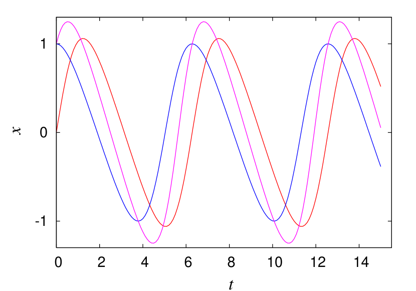
Figure 1: (Color online) Harmonic periodic solutions of the nonlinear Liénard type oscillator for different initial conditions (Eq. (2)) with frequency same as that of the linear harmonic oscillator.

Figure 2: Phase trajectories corresponding to Eq. (2) for $|x|<\frac{3\omega}{k}$: (a) $(x-\dot{x})$ plane, (b) $(x-p)$ plane.

III.2 Lagrangian and Hamiltonian description

The form of the time independent first integral $\mathfrak{I}_{1}$ as given by Eq. (11) suggests that one can indeed give a Lagrangian and so a Hamiltonian description for Eq. (2) when $\lambda_{1}>0$. Indeed we identify a suitable Lagrangian for the system (2) as

$$L=\frac{27\lambda_{1}^{3}}{2k^{2}}\bigg{(}\frac{1}{k\dot{x}+\frac{k^{2}}{3}x^{2}+3\lambda_{1}}\bigg{)}+\frac{3\lambda_{1}}{2k}\dot{x}-\frac{9\lambda_{1}^{2}}{2k^{2}}.$$ (14)

Then the canonically conjugate momentum can be defined as

$$p=\frac{\partial L}{\partial\dot{x}}=-\frac{27\lambda_{1}^{3}}{2k}\bigg{(}\frac{1}{(k\dot{x}+\frac{k^{2}}{3}x^{2}+3\lambda_{1})^{2}}\bigg{)}+\frac{3\lambda_{1}}{2k}.$$ (15)

Consequently, one can obtain the Hamiltonian associated with Eq. (2) as

$$H=\frac{9\lambda_{1}^{2}}{2}\bigg{(}\frac{(\dot{x}+\frac{k}{3}x^{2})^{2}+\lambda_{1}x^{2}}{(k\dot{x}+\frac{k^{2}}{3}x^{2}+3\lambda_{1})^{2}}\bigg{)}\equiv\frac{9\lambda_{1}^{2}\mathfrak{I}_{1}}{2},$$ (16a)

or

$$H=\frac{9\lambda_{1}^{2}}{2k^{2}}\bigg{(}2-2(1-\frac{2kp}{3\lambda_{1}})^{\frac{1}{2}}+\frac{k^{2}x^{2}}{9\lambda_{1}}-\frac{2kp}{3\lambda_{1}}-\frac{2k^{3}x^{2}p}{27\lambda_{1}^{2}}\bigg{)}.$$ (16b)

Note that in the above expressions $L,p$ and $H$, we have kept certain prefactors and constant terms in order to have the correct limits for $k\rightarrow 0$, namely the harmonic oscillator limit.The nature of the trajectories in the $(x-\dot{x})$ and $(x-p)$ planes are shown in Figs. 2. They form closed concentric curves in the region $|x|<\frac{3\omega}{k}$.

Finally we may point out that because of the form of the second and third terms in the right hand side of (14) one may define a modified Lagrangian

$$\bar{L}=\frac{1}{k\dot{x}+\frac{k^{2}}{3}x^{2}+3\lambda_{1}},\qquad\qquad\qquad\qquad\qquad\qquad\qquad\qquad\;\;\qquad\qquad\qquad\qquad$$ (17a)

with the conjugate momentum

$$\bar{p}=-\frac{k}{(k\dot{x}+\frac{k^{2}}{3}x^{2}+3\lambda_{1})^{2}}\qquad\qquad\qquad\qquad\qquad\qquad\qquad\;\;\;\qquad\qquad\qquad\qquad$$ (17b)

and the associated Hamiltonian

$$\bar{H}=\frac{2k\dot{x}+\frac{k^{2}}{3}x^{2}+3\lambda_{1}}{(k\dot{x}+\frac{k^{2}}{3}x^{2}+3\lambda_{1})^{2}}\qquad\qquad\qquad\qquad\qquad\qquad\qquad\quad\;\;\qquad\qquad\qquad\qquad$$ (17c)

or

$$H=\bigg{(}\frac{k}{3}x^{2}+\frac{3\lambda_{1}}{k}\bigg{)}p-2\sqrt{\frac{-p}{k}},\qquad\qquad\qquad\qquad\qquad\qquad\quad\qquad\qquad\qquad\qquad$$ (17d)

which again correspond to the equation of motion (2), provided $k\neq 0$. However in the limit $k\rightarrow 0$, in order to get the correct harmonic oscillator it is preferable to have the forms (14)-(16). On the other hand, the later forms (17) have the advantage that they give interesting $\lambda_{1}=0$ limit, which we discuss in the next section. Consequently, we have chosen to present both the forms here.

IV Unusual features of Eq.(2) with $\lambda_{1}>0$

IV.1 Amplitude independent frequency of oscillations

The remarkable features of the general solution (13) are that the nonlinear system (2) admits harmonic periodic solutions (13) and that the frequency of these periodic oscillations, $\nu=\frac{\omega}{2\pi}=\frac{\sqrt{\lambda_{1}}}{2\pi}$, is completely independent of the amplitude or initial condition, a feature which is generally quite uncommon for nonlinear oscillators of conservative type. The form of the solution is shown in Fig. 1. It may be noted that in the limiting case of vanishing nonlinearity, $k=0$, one recovers the solution of the linear harmonic oscillator as it should be from Eq. (13) and there is no change in the angular frequency $\omega=\sqrt{\lambda_{1}}$ even when $k\neq 0$, as can be seen from Eq. (13). However, it may be noted that in the limit $\lambda_{1}$ or $\omega\rightarrow 0$, $A\rightarrow 0$ and so $x\rightarrow 0$, the trivial solution to (2) and not to the aperiodic bounded solution (3). Thus at $\lambda_{1}=0$, a bifurcation occurs.

IV.2 The nature of flow function

Another interesting feature of Eq. (2) is that when written as a system of two first order equations, it takes the form

$$\dot{x}=y\equiv f_{1}(x,y),$$ (18a)

$$\dot{y}=-kxy-\frac{k^{2}}{9}x^{3}-\lambda_{1}x\equiv f_{2}(x,y).$$ (18b)

For $\lambda_{1}>0$, it has one equilibrium point $(0,0)$ which is of centre type compatible with the occurrence of nonisolated periodic orbits. Interestingly the conventional criterion for conservative systems (see for example Refs. Lit:1983 ; Mcc:1993 ; Dra:1992 ; Nic:1995 ), namely, the value of the divergence of the flow function $\Lambda=\frac{\partial f_{1}}{\partial x}+\frac{\partial f_{2}}{\partial y}$ for Eq. (18) vanish, fails here as $\Lambda=-kx$. Only the average of $\Lambda$, namely

$$\bar{\Lambda}=\frac{1}{T}\int_{o}^{T}\Lambda dt=-\frac{k\omega}{2\pi}\int_{o}^{\frac{2\pi}{\omega}}xdt,$$

on actual evaluation using the solution (13), vanishes. Such a generalized criterion that the average of the flow function vanishes for a conservative system seems to be a necessary condition as the present example shows.

V The aperiodic cases $\lambda_{1}\leq 0$

In the previous section, we discussed the dynamics of (2) for the case $\lambda_{1}>0$. In the following we explore the dynamics of the system (2) with $\lambda_{1}\leq 0$.

For $\lambda_{1}<0$, both the time-dependent integrals (10) are real, from which the explicit solution can be obtained straightforwardly as

$$x(t)=\bigg{(}\frac{3\sqrt{|\lambda_{1}|}(I_{1}e^{2\sqrt{|\lambda_{1}|}t}-1)}{kI_{1}I_{2}e^{\sqrt{|\lambda_{1}|}t}+k{(1+I_{1}e^{2\sqrt{|\lambda_{1}|}t})}}\bigg{)},$$ (19)

where $I_{1}$ and $I_{2}$ are constants. Solution (19) clearly shows the dissipative/damping/aperiodic nature of the system for $\lambda_{1}\leq 0$ in Eq. (2).

We now note that system $\lambda_{1}\leq 0$ still admits the Lagrangian and Hamiltonian descriptions. In fact the Lagrangian $L$ and the Hamiltonian $H$ for the case $\lambda_{1}>0$, namely the forms (14) and (16), respectively, are valid here also. The only difference here is that one has to replace $\lambda_{1}$ with $-|\lambda_{1}|$ in the respective places in Eqs. (14) and (16) for the present case. On the other hand the forms (17) are valid for $\lambda_{1}>0$ as well as $\lambda_{1}\leq 0$, though not valid in the limiting harmonic oscillator case $k\rightarrow 0$.

The major difference in the dynamics comes from the nature of the solution. In the present case it admits decaying type or aperiodic (front like) solutions only, see Fig. 3, where the time of decay or approach to asymptotic value is independent of the amplitude/initial value, which is once again an unusual feature for a nonlinear dynamical system.

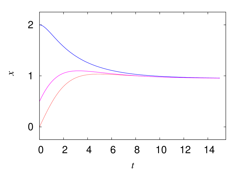
Figure 3: (Color online) Solution plot for case $\lambda_{1}<0$ for different initial conditions.

The nontrivial general solution for the limiting case $\lambda_{1}=0$ is given in Eq. (3). Interestingly in this case also one can deduce a Lagrangian and the associated Hamiltonian, which (from eqs. (17)) turns out to be

$$\hat{L}=\bigg{(}\frac{1}{k\dot{x}+\frac{k^{2}}{3}x^{2}}\bigg{)},$$ (20)

and

$$H=\frac{k}{3}x^{2}p-2\sqrt{\frac{-p}{k}},$$ (21)

where

$$p=-\frac{k}{(k\dot{x}+\frac{k^{2}}{3}x^{2})^{2}}.$$ (22)

The above form of Lagrangian can also be deduced from the form (14), by taking the Lagrangian for the limiting case $\lambda_{1}=0$ as

$$\hat{L}=\lim_{\lambda_{1}\rightarrow 0}\;\frac{2k^{2}}{27\lambda_{1}^{3}}(L-\frac{3\lambda_{1}}{2k}\dot{x}+\frac{9\lambda_{1}^{2}}{2k^{2}}).$$

The expressions $p$ and $H$ given above can be obtained from this $\hat{L}$. The solution plot (corresponding to solution (3)) is given in Fig. 4.

One can also calculate the flow function in the case $\lambda_{1}\leq 0$. Again from Eq. (18) we find that the divergence of the flow function for $\lambda_{1}\leq 0$ is $\Lambda=-kx$. But from the general expression for the solution, one can always choose $x(t)>0$ for all finite $t$. So one might conclude that the system is dissipative (because $\Lambda<0$) inspite of its just proved conservative nature. In order to overcome this incompatibility, and noting that for the case $\lambda_{1}<0$, the dynamical variable $x(t)$ asymptotically tends to a constant value $x(\infty)=\frac{3\sqrt{\lambda_{1}}}{k}$, we again define the condition for conservative flow is that the time average of the divergence of the flow function with reference to the asymptotic $(t\rightarrow\infty)$ value should vanish:

$$\bar{\Lambda} =\lim_{T\rightarrow\infty}\frac{1}{T}\int_{o}^{T}[\Lambda(t)-\Lambda(\infty)]dt=0.$$ (23)

In the present cases, we have

$$\bar{\Lambda} =-\lim_{T\rightarrow\infty}\frac{k}{T}\int_{o}^{T}[x(t)-x(\infty)]dt.$$ (24)

For the case $\lambda_{1}=0$, from the solution (3) we note that $x(\infty)=0$ and $\int_{o}^{T}\Lambda(t)dt=-3\log(1+\frac{kT(2I_{1}+T)}{6I_{2}})$ so that $\bar{\Lambda}=0$ from (24). On the other hand for $\lambda_{1}<0$, $\int_{o}^{T}\Lambda(t)dt=-3\sqrt{\lambda_{1}}T-3\log(\frac{I_{1}+I_{1}I_{2}e^{-T\sqrt{\lambda_{1}}}+e^{-2T\sqrt{\lambda_{1}}}}{(1+I_{1}+I_{1}I_{2})})$ and $\Lambda(\infty)=-3\sqrt{\lambda_{1}}$ so that $\bar{\Lambda}$ vanishes here also.

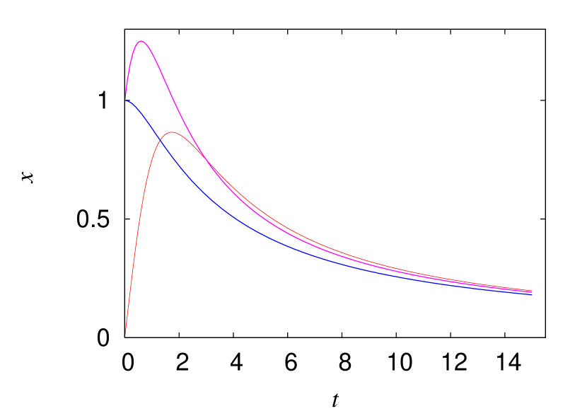
Figure 4: (Color online) Solution plot for case $\lambda_{1}=0$ for different initial conditions.

VI Linearizing and canonical transformations

At this stage one may also try to trace the reason for the existence of the above type of remarkable oscillatory behaviour for Eq. (2). Under the transformation $x=\frac{3\dot{w}}{kw}$, Eq. (2) transforms to a linear third order differential equation,

$$\dddot{w}+\lambda_{1}\dot{w}=0,$$ (25)

from which also one can trace the solution (13). Further, it gets transformed into a free particle equation $X^{\prime\prime}=0$, where prime denotes differentiation with respect to a new variable $\tau$, with the point transformation

$$X=(\frac{k}{3\lambda_{1}}-\frac{1}{\sqrt{-\lambda_{1}}x})e^{-\sqrt{-\lambda_{1}}t},$$

$$\tau=(\frac{k}{3\sqrt{-\lambda_{1}}}-\frac{1}{x})e^{\sqrt{-\lambda_{1}}t}.\qquad$$ (26)

Even then it is very unexpected and unusual to realize such nonlinear oscillator systems having simple properties similar to that of linear oscillators.

In addition to the above, one can also linearize the equation (2) through a nonlocal transformation,

$$U=\displaystyle{xe^{\frac{k}{3}\int x(t^{\prime})dt^{\prime}}}.$$ (27)

Under this transformation Eq. (2) gets modifieed to the form of a linear harmonic oscillator equation,

$$\ddot{U}+\lambda_{1}U=0.$$ (28)

Note that the above transformation (27) is valid for all the three cases, namely, $\lambda_{1}>0,\;\lambda_{1}=0$ and $\lambda_{1}<0$. For $\lambda_{1}>0$, obviously the solution of (28) is

$$U=A\sin(\omega t+\delta),$$ (29)

where $A$ and $\delta$ are arbitrary constants and frequency $\omega=\sqrt{\lambda_{1}}$, which is independent of the amplitude. Consequently, from the forms of the general solutions (29) and (13) we can identify the obvious canonical transformation

$$x=\frac{U}{1-\frac{k}{3\lambda_{1}}P},$$ (30)

where $P=\dot{U}$, so that using eq. (15) for the canonically conjugate momentum $p$, we have

$$p=P(1-\frac{k}{6\lambda_{1}}P).$$ (31)

It is straightforward to check that when $U$ and $P$ are canonical so do $x$ and $p$ (and vice versa) and that the Hamiltonian $H$ in eq. (16) can be rewritten as the standard linear harmonic oscillator Hamiltonian

$$H=\frac{1}{2}(P^{2}+\lambda_{1}U^{2}).$$ (32)

More interestingly, even for $\lambda_{1}<0$, making use of similar argument for the aperiodic bounded solution (19), we can write the canonical transformation

$$x=\frac{U}{1+\frac{k}{3\lambda_{1}}P},\qquad\;\;p=P(1+\frac{k}{6\lambda_{1}}P),$$ (33)

where $P=\dot{U}$, so that the Hamiltonian (16) (for $\lambda_{1}<0$) is mapped on to the unbounded (wrong sign) linear harmonic oscillator

$$H=\frac{1}{2}(P^{2}-\omega^{2}U^{2}),\;\;\;\omega=\sqrt{|\lambda_{1}|}.$$ (34)

Finally for the $\lambda_{1}=0$ case, we can identify the canonical transformation

$$x=\frac{3P}{kU},\qquad\;\;p=-\frac{kU^{2}}{6},$$ (35)

so as to transform to a freely falling particle Hamiltonian $H=\frac{P^{2}}{2}-\sqrt{\frac{2}{3}}U$. However, we suspect that there may exist a canonical transformation for this specific case $\lambda_{1}=0$, which will take the corresponding form of Eq. (2) to a free particle, though we could not succeed to find it so far.

Of course, it is well known that linearization in general does not ensure preservation of properties of linear systems in the nonlinear case. The classical example is the Cole-Hopf transformation through which the nonlinear Burgers equation is transformed into the linear heat equation Lak:2003 . This is also true in the case of various soliton equations such as Korteweg-de Vries, sine-Gorden, nonlinear Schr$\ddot{o}$dinger and other equations which are all linearizable in certain sense. Nevertheless in the present example of Eq. (2), the amplitude independence of frequency does indeed get preserved. These considerations also raise the question of identifying the most general class of nonlinear dynamical systems of the form $\ddot{x}=f(x,\dot{x},t)$ that has solutions whose frequency is independent of the amplitude as in the case of the linear harmonic oscillator, a point which is under study presently.

VII Generalization and other examples

VII.1 Generalization

We also observed that the above exceptional properties admitted by Eq. (2) is also common for a class of nonlinear systems. In particular we find that the modified Emden type equation with linear term and constant external forcing

$$\ddot{x}+(k_{1}x+k_{2})\dot{x}+\frac{{k_{1}}^{2}}{9}x^{3}+\frac{k_{1}k_{2}}{3}x^{2}+\lambda_{1}x+\lambda_{2}=0,$$ (36)

where $k_{1},k_{2},\lambda_{1}$ and $\lambda_{2}$ are parameters, for which also one can obtain similar propertes as discussed above for Eq. (2) when the parameters satisfy the specific condition $\lambda_{1}=\frac{2k_{2}^{2}}{9}+\frac{k_{1}\lambda_{2}}{k_{2}}$. To be specific, for the case $\frac{k_{1}\lambda_{2}}{k_{2}}-\frac{k_{2}^{2}}{9}>0$, the explicit periodic solution takes the form

$$\bar{x}(t)=\frac{A\sin{(\bar{\omega}t+\delta)}}{1-(\frac{k}{3\bar{\omega}})A\cos{(\bar{\omega}t+\delta)}},\qquad\qquad\qquad$$

$$\qquad\qquad 0\leq A<\frac{3\bar{\omega}}{k},\qquad\bar{\omega}=\sqrt{\lambda_{1}-\frac{k_{2}^{2}}{3}},$$ (37)

where $\bar{x}(t)=x(t)+\frac{k_{2}}{k_{1}}$. For $\frac{k_{1}\lambda_{2}}{k_{2}}-\frac{k_{2}^{2}}{9}<0$, the system becomes aperiodic.

VII.2 Comparison with other nonlinear oscillators

Finally, it is of interest to compare the dynamics of Eq. (2) with another interesting nonlinear oscillator Lak:2003 ; Mat:1974 of the form

$$\ddot{x}-\frac{\lambda x\dot{x}^{2}}{1+\lambda x^{2}}+\frac{\omega_{0}^{2}x}{1+\lambda x^{2}}=0,$$ (38)

which possesses exact periodic solution $x(t)=A\sin(\Omega t+\delta)$, where the frequency $\Omega=\frac{\omega_{0}}{\sqrt{1+\lambda A^{2}}}$, exhibiting the characteristic amplitude-dependent frequency of nonlinear oscillators inspite of the sinusoidal nature of the solution Eq. (38). Equation (38) has a natural generalization in three dimensions Lak:1976 and these systems can be also quantized exhibiting many interesting features and can be interpreted as an oscillator constrained to move on a three-sphere Hig:1976 . Several generalizations of these systems to $N$-degrees of freedom are also possible Senthil . But all these nice properties are subject to the fact that the frequency is amplitude-dependent. It is only Eq. (2) which admits the amplitude independence property of frequency for a nonlinear oscillator. Studies of such systems will have important implications in developing nonlinear systems whose frequency remain unchanged even with the addition of suitable nonlinearity. Also, Eq. (38) when written as a system of two first order equations of the form (18), with

$$f_{1}(x,y)=y\qquad\mbox{and}\quad\qquad f_{2}(x,y)=\frac{\lambda xy^{2}}{1+\lambda x^{2}}-\frac{\omega_{0}^{2}x}{1+\lambda x^{2}},$$

the divergence of the flow function $\Lambda=\frac{2\lambda xy}{1+\lambda x^{2}}\neq 0$. On the other hand Eq. (38) is also a Hamiltonian system Mat:1974 with the Hamiltonian given by

$$H=\frac{1}{2}[p^{2}(1+\lambda x^{2})+\frac{\omega_{0}^{2}x}{1+\lambda x^{2}}],$$

eventhough $\Lambda\neq 0$. Once again it is only

$$\bar{\Lambda}=\frac{1}{T}\int_{o}^{T}\frac{2\lambda xy}{1+\lambda x^{2}}dt=0.$$

This again confirms that for a conservative system it is necessary that the average of the divergence of the flow function vanish.

VIII Conclusion

In this work, we have identified a nonlinear oscillator which exhibits unusual oscillatory properties: Purely harmonic oscillation whose frequency is completely independent of the amplitude and is the same as that of the linear harmonic oscillator. The conservative Hamiltonian nature of the system has been established, which also necessitates the generalization of the definition of conservative systems in terms of the divergence of the flow function. Further, even for an apparently dissipative type/aperiodic (front like) type system, the Hamiltonian structure is preserved and the definition of the conservative system in terms of the divergence of flow function needs to be generalized. We believe identification of such nonlinear systems having the basic property of linear systems will have considerable practical application as the effect of higher harmonics is completely suppressed. Also it is of interest to consider the quantum mechanical version of the system (16) and its higher dimensional generalizations as well as the effect of external forcing and additional damping, which are being pursued.

We have also shown that Eq. (2) admits certain interesting geometrical properties. For example, under the invertible point transformation (26), Eq. (2) gets transformed to the free particle equation whereas with the appropriate choice of canonical transformations one can transform it to a simple harmonic oscillator (or to an unbounded oscillator or to a freely falling particle depending on the value of the parameter $\lambda_{1}$) equation. Interestingly, the very same nonlinear oscillator can also be transformed to a third order linear equation through a nonlocal transformation, while yet another nonlocal transformation transforms it to a linear harmonic oscillator. As far as our knowledge goes no such single nonlinear oscillator possesses such large class of transformation properties. We believe that exploring such nonlinear equations will be highly rewarding in understanding nonlinear systems and further work is in progress in this direction.

- (1) A. H. Nayfeh and D. T. Mook, Nonlinear Oscillations, (John Wiley & Sonc. Inc, 1979).
- (2) J. Guckenheimer and P. Holmes, Nonlinear Oscillations, Dynamical Systems and Bifurcations of Vector Fields, (Springer-Verlag, New York, 1983).
- (3) M. Tabor, Chaos and Integrability in Nonlinear Dynamics: An Introduction, (John Wiley & Sonc. Inc, 1989).
- (4) S. Wiggins, Introduction to Applied Nonlinear Dynamical Systems and Chaos, (Springer-Verlag, New York, 2003).
- (5) M. Lakshmanan and S. Rajasekar, Nonlinear Dynamics: Integrability, Chaos and Patterns, (Springer-Verlag, New York, 2003).
- (6) S. Chandrasekhar, An Introduction to the Study of Stellar Structure, (Dover, New York, 1957); J. M. Dixon and J. A. Tuszynski, Phys. Rev. A 41, 4166 (1990).
- (7) F. M. Mahomed and P. G. L. Leach, Quaestiones Math. 8, 241 (1985); 12, 121 (1989); P. G. L. Leach, J. Math. Phys 26, 2510 (1985); P. G. L. Leach, M. R. Feix and S. Bouquet, J. Math. Phys 29, 2563 (1988).
- (8) M. Prelle and M. Singer, Trans. Am. Math. Soc. 279, 215 (1983); L. G. S. Duarte, S. E. S. Duarte, A. C. P. da Mota and J. E. F. Skea, J. Phys. A 34, 3015 (2001).
- (9) V. K. Chandrasekar, M. Senthilvelan and M. Lakshmanan 2005 Proc. R. Soc. London (arXiv:nlin. SI/0408053, accepted for publication).
- (10) A. J. Litchenberg and M. A. Lieberman, Regular and Stochastic Motion, (Springer-Verlag, New York, 1983).
- (11) J. L. McCauley, Chaos, Dynamics and Fractals: An Algorithmic Approach to Deterministic Chaos, (Cambridge University Press, 1993).
- (12) P. G. Drazin, Nonlinear Systems, (Cambridge University Press, 1992).
- (13) G. Nicolis, Introduction to Nonlinear Science, (Cambridge University Press, 1995).
- (14) P. M. Mathews and M. Lakshmanan, Quart. Appl. Math. 32, 215 (1974).
- (15) M. Lakshmanan and K. Eswaran, J. Phys. A 8, 1658 (1975).
- (16) P. W. Higgs, J. Phys. A 12, 309 (1979).
- (17) J. F. Carinena, M. F. Ranada, M. Santander and M. Senthilvelan, Nonlinearity 17, 1941 (2004).