Allelomimesis as universal clustering mechanism
for complex adaptive systems

Abstract

Animal and human clusters are complex adaptive systems and many are organized in cluster sizes $s$ that obey the frequency-distribution $D\left(s\right)\propto s^{-\tau}$. Exponent $\tau$ describes the relative abundance of the cluster sizes in a given system. Data analyses have revealed that real-world clusters exhibit a broad spectrum of $\tau$-values, $0.7\textrm{ (tuna fish schools)}\leq\tau\leq 2.95\textrm{ (galaxies)}$. We show that allelomimesis is a fundamental mechanism for adaptation that accurately explains why a broad spectrum of $\tau$-values is observed in animate, human and inanimate cluster systems. Previous mathematical models could not account for the phenomenon. They are hampered by details and apply only to specific systems such as cities, business firms or gene family sizes. Allelomimesis is the tendency of an individual to imitate the actions of its neighbors and two cluster systems yield different $\tau$ values if their component agents display different allelomimetic tendencies. We demonstrate that allelomimetic adaptation are of three general types: blind copying, information-use copying, and non-copying. Allelomimetic adaptation also points to the existence of a stable cluster size consisting of three interacting individuals.

I Introduction

Huge amounts of data have been collected and analyzed by researchers in various fields of the natural and social sciences concerning the clustering behavior of animals (fish schools, buffalo herds, etc). In the real world, a number of different cluster types often exist and share common habitat and an accurate understanding of cluster formation among diverse animate and inanimate systems is of great value in wildlife preservation, environmental management, urban planning, economics, genetics and even politics.

Animal and human clusters are complex systems with adaptive agents. Many exist in cluster sizes $s$ that obey the frequency distribution $D\left(s\right)\propto s^{-\tau}$. Exponent $\tau$ determines the relative abundance of the cluster sizes – a small $\tau(\approx 0)$ implies equal abundance of large and small clusters in a given system. Power-law distributions indicate the role of self-organization during cluster formation and the presence of scale-free interaction dynamics that holds over several scales of the agent population and size of interaction space Bak (1996); Stanley et al. (1996).

Scale-free clusters have been observed with gene families, colloids, fish schools, slum areas, city populations, business firms, and galaxies to name a few. Table 1 lists forty-five different real-world cluster systems with their measured $\tau$ values ranging from $\tau=0.7$ (tuna fish schools) Bonabeau and Dagorn (1995); Bonabeau et al. (1999) to $\tau=2.95$ (galaxy clusters) Jarrett (1998).

To our knowledge, no mathematical model can generate size-frequency distributions that cover the entire range of $\tau$-values in Table 1. Available models are effective only at describing particular systems such as cities Stanley et al. (1996); Johansson (1997), firms Axtell (2001), or gene families Huynen and van Nimwegen (1998). Current models utilize many interaction details that limit the range of their applicability May (2004).

Here, we show that allelomimesis is a fundamental mechanism for adaptation that can accurately explain why real-world cluster systems exhibit a broad spectrum of $\tau$-values. Allelomimesis is the act of copying one’s kindred neighbors Parrish and Edelstein-Keshet (1999); Juanico et al. (2003). We demonstrate that differences in $\tau$-values are caused from variations in allelomimetic behavior (described by a single parameter $\alpha$ where $0\leq\alpha\leq 1$) of the agent phenotypes from one cluster system to another. We derive a nonlinear relation between $\tau$ and $\alpha$ that rationalizes the distribution of $\tau$ values in animal, human, and inanimate cluster systems. For strongly- allelomimetic agents ($\alpha\approx 1$), clustering by allelomimesis predicts a stable cluster size at $s=3$ which has been observed previously in marmots Grimm (2003) and killer whales Baird and Dill (1996).

Our clustering model unifies previous mathematical models of cluster formation towards a common starting point. Allelomimesis is expressed in various (higher-order) forms in previous self-aggregation models. In animal aggregation models, it is manifested as biosocial attraction Bonabeau et al. (1999) or as conspecific copying Wagner and Danchin (2003). For example, herding which has been observed in panicking mice escaping from a two-door enclosure is a striking example of nearest- neighbor copying Saloma et al. (2003). In the percolation model of urban growth, allelomimesis is implicit in the concept of correlation Makse et al. (1995). The tendency of employees to associate with those that belong to the same income bracket in Axtell’s model of firms Axtell (2001) can also be construed as another expression of allelomimesis.

Copying is natural among social groups and is an evolutionary mechanism in human societies Higgs (2000). In a community of strongly allelomimetic individuals, it is natural to expect that full cooperation is achieved quickly without the threat of punishment Milinski et al. (2002). In gene families, cluster formation is explained as an intricate birth-death process Huynen and van Nimwegen (1998). In olivine crystal sizes, it is driven by complicated tectonic processes Armienti and Tarquini (2002).

Allelomimetic interaction between agents could be described with few simple local rules Juanico et al. (2003). A single measure $\alpha$ is sufficient to vary the exponent $\tau$ over a wide range of values. Agents search for neighbors (kindreds) and those that are strongly-allelomimetic ($\alpha\approx 1$) are likely to copy their neighbors leading to the formation of relatively large clusters such as those observed in fish schools (see Table 1). On the other hand, relatively large clusters are highly unlikely in gene families, colloids, and galaxies which are systems with components that are incapable of copying each other ($\alpha\approx 0$).

Of particular interest are human cluster systems such as slums of informal settlers, cities, and business firms. Table 1 reveals that such systems occupy a narrow band of the $\tau$-spectrum ($1.4\leq\tau\leq 2.16$). Unlike other animals, humans are rational and capable of deciding on their own based upon a set of competing factors that promote individual self-interest on the one hand and collective benefit on the other. We determine the possible classes of allelomimetic interactions by establishing a quantitative relation between $\alpha$ and $\tau$.

Our presentation proceeds as follows: In Sec. II we describe briefly our mathematical model for clustering by allelomimesis while in Sec. III we compare the predictions of the model with those observed in real-world clusters such as those listed in Table 1. We end our presentation by discussing the results of our comparison.

II Methodology

Table 1: Measured $\tau$-values of real-world cluster systems with power-law $D\left(s\right)$ plots. Also shown are the corresponding values of the allelomimesis measure $\alpha$.

REAL-WORLD CLUSTER SYSTEM	$\tau$	$\alpha$
Tuna near fish-aggregating device Bonabeau and Dagorn (1995); Bonabeau et al. (1999)	$0.70$	$0.9895$
Clupeid fish Sardinella maderensis & S. aurea Bonabeau and Dagorn (1995); Bonabeau et al. (1999)	$0.95$	$0.9895$
Alpine marmot Marmota marmota Grimm (2003)	$1.08\pm 0.25$	$0.9895$
African bufallo Syncerus cafer Bonabeau et al. (1999)	$1.15$	$0.9894$
Wasps Ropalidia fasciata Ito et al. (2002)	$1.19\pm 0.008$	$0.9893$
Tephritid flies Sjoberg et al. (2000)	$1.37$	$0.9888$
Free-swimming tuna with three species mixed Bonabeau and Dagorn (1995); Bonabeau et al. (1999)	$1.49$	$0.9877$
Spatial sizes of forest fires Malamud et al. (1998)	$1.5$	$0.9877$
Offshore-spotted dolphin Stenella attenuata Perkins and Edwards (1997)	$1.79\pm 0.05$	$0.9590$
Three species of African baboons Altmann and Altmann (1970)	$2.01\pm 0.08$	$0.7841$
West Indian manatee Trichecus manatus Kadel et al. (1991)	$2.19\pm 0.07$	$0.4009$
Nomadic Serengeti cheetah Acinonyx jubatus Schaller (1972)	$2.49\pm 0.35$	$0.0378$
Nomadic Serengeti lion Panthera leo Schaller (1972)	$2.49\pm 0.08$	$0.0379$
Mathare valley squatter settlements, Kenya Sobreira and Gomes (2001)	$1.40\pm 0.20$	$0.9888$
Recife squatter settlements, Brazil Sobreira and Gomes (2001)	$1.60\pm 0.20$	$0.9844$
French manufacturing firms in 1962 van Ark and Monnikhof (1996)	$1.84\pm 0.08$	$0.9411$
Japanese manufacturing firms in 1975 van Ark and Monnikhof (1996)	$1.90\pm 0.04$	$0.9067$
Urban agglomerations, India Brinkhoff (2004)	$1.93\pm 0.002$	$0.87$
Towns surrounding London in 1981 Stanley et al. (1996); Makse et al. (1995)	$1.96$	$0.8514$
Towns surrounding Berlin in 1981 Stanley et al. (1996); Makse et al. (1995)	$1.98$	$0.8270$
Swedish firms in 1993 Johansson (1997)	$1.98\pm 0.08$	$0.8270$
Urban areas in Great Britain in 1981 & 1991 Makse et al. (1995)	$2.03$	$0.7512$
City populations in Brazil in 1991 & 1993 Brinkhoff (2004)	$2.04\pm 0.06$	$0.7329$
Urban agglomerations in Russia in 1994 Brinkhoff (2004)	$2.04\pm 0.06$	$0.7285$
Urban agglomerations in U.S.A. in 1994 Brinkhoff (2004)	$2.04\pm 0.07$	$0.7250$
Urban agglomerations in France in 1982 & 1990 Brinkhoff (2004)	$2.05\pm 0.00$	$0.7049$
U.S. firms in 1997 Axtell (2001)	$2.06\pm 0.05$	$0.6974$
City populations in Mexico in 1990 Brinkhoff (2004)	$2.07\pm 0.00$	$0.6814$
City populations in China in 1990 Brinkhoff (2004)	$2.11\pm 0.00$	$0.5970$
World’s most populous cities in 2002 Brinkhoff (2004)	$2.11\pm 0.08$	$0.5959$
British business/manufacturing firms in 1955 Simon and Bonini (1958)	$2.11$	$0.5881$
City populations in Germany in 1994 Brinkhoff (2004)	$2.15\pm 0.20$	$0.5033$
City populations in Japan in 1994 Brinkhoff (2004)	$2.16\pm 0.09$	$0.4692$
Gene family sizes of M. pneumoniae Huynen and van Nimwegen (1998)	$2.69$	$0.0056$
Gene family sizes of S. cerevisiae Huynen and van Nimwegen (1998)	$2.81$	$0.0018$
Gene family sizes of E. coli Huynen and van Nimwegen (1998)	$2.84$	$0.0013$
Gene family sizes of Synechocystis sp. Huynen and van Nimwegen (1998)	$3.17$	$0.0001$
Gene family sizes of H. influenzae Huynen and van Nimwegen (1998)	$3.27$	$0.0000$
Gene family sizes of M. janaschii Huynen and van Nimwegen (1998)	$3.62$	$0.0000$
Gene family sizes of Vaccinia virus Huynen and van Nimwegen (1998)	$3.80$	$0.0000$
Gene family sizes of M. genitalum Huynen and van Nimwegen (1998)	$4.02$	$0.0000$
Gene family sizes of T4 bacteriophage Huynen and van Nimwegen (1998)	$4.61$	$0.0000$
Olivine crystal sizes of GP45 - granoblastic Armienti and Tarquini (2002)	$2.83\pm 0.16$	$0.0015$
Olivine crystal sizes of GP30 - coarse Armienti and Tarquini (2002)	$3.03\pm 0.18$	$0.0002$
Olivine crystal sizes of LANZ3 - porphyroclastic Armienti and Tarquini (2002)	$3.81\pm 0.41$	$0.0000$
Database of 8,000 galaxy clusters Jarrett (1998)	$2.95\pm 0.36$	$0.0005$

II.1 Agent-based model of allelomimetic interaction

An $N\times N$ lattice with free boundaries Domb (1973) is utilized as a platform for our agent-based model of cluster formation. Initially at time step $q_{0}=0$, the lattice cells are empty and for every subsequent time step $q$, an agent is injected into a randomly-selected vacant cell. An agent at cell location $\left(x,y\right)$ is assigned a state $\Psi_{m}\left(x,y\right)$ that is taken from a set of possible states $\left\{\Psi_{m}\right\}=\left\{1,2,\ldots,M\right\}$. State $\Psi\left(x,y\right)$ represents a particular trait, preference, action or any other social attribute that characterize an agent at any given time. For example, $\left\{\Psi_{m}\right\}$ could be different species of tuna swimming within the same field of observation Bonabeau and Dagorn (1995) or the different types of behavior in groups of lions (e.g., hunting, sleeping, yawning, etc.) as described by Schaller Schaller (1972). An empty cell is assigned the value of $\Psi=0$.

An agent at $\left(x,y\right)$ searches for other agents of similar state by occupying the next available cell of its Moore neighborhood which consists of the agent’s eight nearest cells at locations, $\left\{\left(x+j,y+k\right)\right\}$, where indices $i,j=-1,0,1$. The location $\left(x+0,y+0\right)=\left(x,y\right)$ represents the current (default) location of the agent. In deciding to occupy a neighboring cell $\left(x+j,y+k\right)$ in the next time step $q+1$, the agent evaluates the viability of its current position $\left(x,y\right)$ with those of its neighboring cells using the discrete potential function $\Phi$,

$$\Phi\left(x+j,y+k\right)=100\left\{1-\delta\left[\Psi\left(x+j,y+k\right)\right]\right\}-\delta\left[\Psi\left(x+j,y+k\right)\right]\sum_{u,v}\left\{2\delta\left[\Psi\left(x,y\right)-\Psi\left(x+j+u,y+k+v\right)\right]\right\}$$ (1)

where $\delta\left(w\right)$ is the Dirac delta function which is non-zero and equal to unity only when $w=0$. The summation in Eq. 1 is taken from $u=-1,v=-1$ to $u=1,v=1$ and the possible values for $u$ and $v$ are, $-1,0,1$.

The potential barrier $\Phi\left(x+j,y+k\right)$ is highest at $100$ when $\Psi\left(x+j,y+k\right)\neq 0$ which happens when the cell at $\left(x+j,y+k\right)$ is unavailable for occupation. On the other hand, $\Phi\left(x+j,y+k\right)$ becomes much less than 100 when $\Psi\left(x+j,y+k\right)=0$ which is the case when the cell at location $\left(x+j,y+k\right)$ is vacant.

The set of cells $\left\{\left(x+j+u,y+k+v\right)\right\}$ represents the Moore neighborhood of the agent’s neighboring cell $\left(x+j,y+k\right)$. The term, $\delta\left[\Psi\left(x,y\right)-\Psi\left(x+j+u,y+k+v\right)\right]$ is a comparison between $\Psi\left(x,y\right)$ with those in the Moore neighborhood of the vacant cell at $\left(x+j,y+k\right)$. It is equal to unity when $\Psi\left(x,y\right)=\Psi\left(x+j+u,y+k+v\right)$. More details of the model may be found elsewhere Juanico et al. (2003).

Eq. 1 is applied to every cell in the Moore neighborhood and the agent occupies the vacant cell that yields the lowest (most negative) value for $\Phi$, expressed in the following minimum condition:

$$\Phi_{min}=\min_{j,k}\Phi\left(x+j,y+k\right)$$ (2)

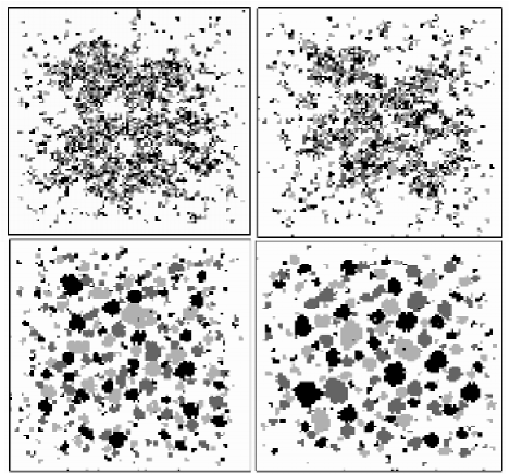
Figure 1: Typical configurations of agents with $\alpha=0$ (first row, first column), 0.5 (first row, second column), 0.99 (second row, first column) and 0.995 (second row, second column) after $q_{T}=600,000$ iterations ($N=100$). Different gray-levels represent three ($M=3$) possible states of an agent.

If more than one cell satisfies Eq. 2, then the agent randomly selects among these cells. Successive application of the above-mentioned mechanism for a sufficiently long period of time gives rise to clustered configurations such as those in Fig. 1. A cluster is defined as a contiguous group of agents of the same state $\Psi$ that are connected via neighboring cells.

The tendency to copy its neighbors can vary from one agent phenotype to another. We use a single parameter $\alpha$ to describe different levels of allelomimetic behavior where, $0\textrm{ (non-allelomimetic)}\leq\alpha\leq 1\textrm{ (blind copying)}$. The state of a completely allelomimetic agent ($\alpha=1$) always depends on the condition of its Moore neighborhood while that of a non-allelomimetic agent is oblivious of the states of its Moore neighborhood. For computational simplicity, we assume that all the agents in the lattice have the same $\alpha$ value. Agent segregation and clustering are attributed directly to local behavior of the individual agents instead of a globally-defined probability of segregation and clustering Bonabeau and Dagorn (1995).

Let $\zeta$ be a random variable taken from a uniform distribution between 0 and 1. If $\zeta>\alpha$, then an agent randomly selects a state from the set $\left\{\Psi_{m}\right\}$. On the other hand, if $\zeta\leq\alpha$, then the agent’s state is set by its Moore neighborhood such that the state with the highest occurence within the neighborhood is the one copied by the agent. If more than one state satisfies this condition, then the agent selects randomly from among these states.

To avoid completely filling the lattice through the constant addition of agents, we also include a constant probability of death for each agent. The death probability is held sufficiently low (1 in 10,000 for every time step) to maintain a relatively high lattice population density $\rho$. When an agent dies, its cell location becomes empty in the next time step. The agent population density $\rho$ in the lattice remains increasing with $q$ and agents are more likely to stay in its original position after a sufficiently long period of time where number of available vacant cells in its Moore neighborhood becomes smaller.

Each simulation is run for a time-step duration of $q_{T}=600,000$ which is sufficient to allow the agent population density to reach a steady-state value, $\rho\left(q_{T}\right)\approx 0.5$. To incrase the probability of conspecific agents meeting and coalescing within a reasonably short period of computational time, we choose $M=3$, i.e., $\left\{\Psi_{m}\right\}=\left\{1,2,3\right\}$. The choice of $M=3$ is consistent with the dimensional reduction hypothesis of Bonabeau et. al. Bonabeau et al. (1999) which states that clustering is more likely at low effective dimensions. We also mentioned that interesting clustering behavior has been observed in real-world systems wherein three different species of individuals are mixed within the same territory Bonabeau and Dagorn (1995); Bonabeau et al. (1999); Altmann and Altmann (1970).

Fig. 1 presents typical configurations of a cluster system ($M=3$) at different $\alpha$ values. A relatively high local density of agents is found in the lattice interior due to the “free” boundary condition which eliminates all agents that wander beyond the lattice boundaries. We measure the cluster size $s$ (in cell units) using the Hoshen-Kopelman algorithm Hoshen and Kopelman (1976). A histogram ($\textrm{bin size}=1$) of the average cluster sizes is calculated for every $\alpha$-value using 10 trials. The cluster-size distribution is fitted by a power-law function over a finite range of sizes, $s_{min}\leq s\leq s_{max}$, where $s_{min}$ and $s_{max}$ are the minimum and maximum cluster size, respectively. We determine the $\tau$ value from the best fit curve and use it to characterize the cluster-size distribution. Table 2 presents the relation between the allelomimesis measure $\alpha$ with exponent $\tau$.

We also determine the average duration $\left<Q\right>$ that an agent remains in a particular state and correlate it with the cluster size to which the agent belongs. $\left<Q(s)\right>$ is the amount of time that an agent stays in a cluster of size $s$. It can serve as a rough measure of cluster stability.

II.2 Data from Real-World Cluster Systems

The predictions of our model are compared with measurements taken from different real-world scale-free cluster systems (see Table 1). In our model, group dynamics is confined within a two-dimensional plane which is applicable to real-world clusters formed by human beings and terrestrial animals. Our model remains valid even to fishes which have been found not to utilize fully the three-dimensional character of oceanic space Bonabeau et al. (1999).

Cluster-size distributions are normally taken from direct-count observations and presented as absolute frequency $D\left(s\right)$ plots when the number of data points is sufficiently large, or as cumulative-frequency plots when the data set is sparse. To within a pre-defined accuracy, both methods yield the same $\tau$ value of the $D\left(s\right)$ plot. Cluster-size data from different kinds of animals are presented commonly as direct-count values and data reliability depends heavily on the accuracy of spotting the correct number of members in an animal group. Data on free-swimming tuna, buffalo, and clupeid fish are taken from Bonabeau’s study Bonabeau and Dagorn (1995); Bonabeau et al. (1999) while those of Serengeti lions and cheetahs were sourced from Schaller Schaller (1972). Information on baboons is accrued from several separate studies by Altmann and Altmann Altmann and Altmann (1970) on three different baboon species. Marmot data were quoted from Grimm et. al. Grimm (2003). Cluster data about dolphins and manatee were obtained from direct-counting and their reliability was limited by visibility.

Information about city populations and slum areas were taken from Brinkhoff Brinkhoff (2004) and Sobreira and Gomes Sobreira and Gomes (2001), respectively. The available data sets were plotted as a cumulative frequency distribution, $C\left(\geq s\right)=\sum_{s^{\prime}}N\left(s^{\prime}\right)$, where $N\left(s^{\prime}\right)$ are the number of clusters of size $s^{\prime}$. The summation is taken from $s^{\prime}=s$ to the largest available cluster size $s_{max}$. Exponent $\tau$ is calculated using the property of power-law distributions which states that if $\tau^{\prime}$ is the exponent of $C\left(\geq s\right)$ then it follows that $\tau=\tau^{\prime}+1$ Burroughs and Tebbens (2001). Data about the employee sizes of U.S. firms were taken from Axtell Axtell (2001) while those from Swedish, Japanese and British firms were obtained from Johansson Johansson (1997) and Simon and Bonini Simon and Bonini (1958), respectively.

We also studied cluster size data of inanimate systems ($\alpha\approx 0$) such as gene families in various kinds of bacteria Huynen and van Nimwegen (1998), olivine crystal sizes in xenoliths of the lithospheric mantle Armienti and Tarquini (2002), and galaxy clusters Jarrett (1998).

III Experimental Results

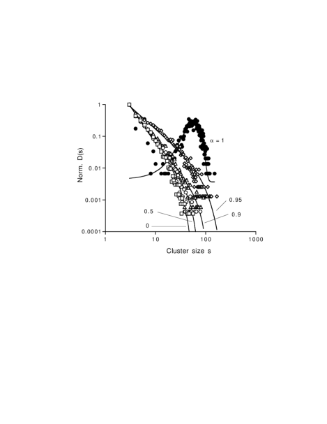
Figure 2: Agent-based modeling ($N=100,M=3$). $D\left(s\right)$ plots for different $\alpha$ values. Solid lines represent data fits with Fischer scaling function.

Fig. 2 shows plots of normalized cluster-size frequency distributions, $D\left(s\right)=N\left(s\right)/N\left(s_{min}\right)$, for different $\alpha$ values ($0\leq\alpha\leq 0.996$). Simplex projection curve fits are derived (solid lines) using the Fischer scaling function Bauer (1988), $F\left(s\right)=As^{-\tau}\exp\left(-bs_{c}\right)$, where $s_{c}$ is the cutoff size, $A$ and $b$ are constants and $s_{min}=3\leq s\leq s_{c}$. Sizes $s=1$ and $s=2$ are excluded from the curve fitting procedure to minimize deviations from the power-law distribution caused by boundary effects and finite agent population. Note that the $D\left(s\right)$ plot obtained with $\alpha=1$ is Gaussian-like with a characteristic size at $s\approx 56$.

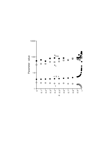
Figure 3: Agent-based modeling, exponent $\tau$ (circles), mean cluster size $\left<s\right>$ (filled circles), cutoff-size $s_{c}$ (squares) and maximum cluster size $s_{max}$ (filled squares) versus the allelomimesis measure $\alpha$.

Fig. 3 plots the dependence of $\tau$ with $\alpha$ (circles) which shows that $\tau$ is independent of $\alpha$ for $\alpha<0.9$. However, as $\alpha\rightarrow 1$, $\tau$ rapidly decreases to zero indicating a nonlinear relation between $\tau$ and $\alpha$. Also shown is the dependence of the mean cluster size $\left<s\right>=M_{1}/M_{0}$, with $\alpha$ (filled circles) where $M_{0}$ and $M_{1}$ are the zeroth- and first-order moments of the size distribution $N\left(s\right)$, respectively.

The sharp variation of $\tau$ and $M_{1}/M_{0}$ as $\alpha\rightarrow 1$ implies a rapid increase in clustering among agents, hence, a greater probability of the formation of large clusters. Fig. 3 also plots $s_{c}$ (squares) and $s_{max}$ (filled squares) as a function of $\alpha$ that also reveal rapid and nonlinear increases for both parameters as $\alpha\rightarrow 1$. The plot behavior of $\tau$, $M_{1}/M_{0}$, $s_{c}$ and $s_{max}$ against $\alpha$ consistently indicate that strongly-allelomimetic agents are capable of forming large, compact and considerably stable associations.

Fig. 4 plots the pair of $\alpha$-$\tau$ values that were generated using our agent-based model. The nonlinear $\alpha\left(\tau\right)$ curve strongly approximates a Fermi distribution,

$$\alpha\left(\tau\right)=\gamma\left\{1+\exp\left[\beta\left(\tau-\tau_{c}\right)\right]\right\}^{-1}$$ (3)

with $\gamma\approx 1$, $\beta=0.104$ and $\tau_{c}=2.15$. Also plotted in Fig. 4 are the measured $\tau$ values (filled circles) from thirty-two selected real-world cluster systems in the order presented in Table 1.

The corresponding $\alpha$ is interpolated from the given measure $\tau$ value of a real-world cluster system via Eq. 3 (reduced $\chi^{2}=0.00529$; $R^{2}=0.9565$). The behavior of Eq. 3 hints to the presence of three general types of allelomimetic interactions, 1) Blind allelomimesis ($\alpha\approx 1$) where agents are most likely to copy conspecifics, 2) Information-use allelomimesis ($\alpha\propto\tau$) where agents are deliberate in their decisions to copy conspecifics, and 3) Non-allelomimetic ($\alpha\approx 0$) where agents do not possess the social attribute to copy their neighbors.

Our findings are consistent with the experiment-based classifications proposed earlier by Wagner and Danchin Wagner and Danchin (2003). Information-use copying may be considered an advance (evolutionary) trait found in humans. It plays a critical role in the expansion of business firms and cities Axtell (2001); Makse et al. (1995). Interestingly, our model indicates that the growth of slum areas is driven by blind copying rather than deliberate decisions based on available information.

Many animal clusters (e.g., fish schools, buffalos) benefit from blind copying ($0.98<\alpha<0.99$). Herding is more likely to emerge quickly in systems with strongly-allelomimetic agents. On the other hand, baboons have a relatively low $\alpha$ at $0.78$ because they live in heirarchical societies Altmann and Altmann (1970) where higher-ranked individuals are more likely to succeed in imposing their will on others below them – allelomimesis is biased towards dominance. The West Indian manatee have a relatively low $\alpha$ of $0.40$ because they are solitary animals Kadel et al. (1991) and are unlikely to encounter other individuals of the same kind within their lifetime. Cheetahs and lions both have low $\alpha$ of $0.038$ because they are nomadic and prefer to hunt alone or in small packs Schaller (1972). In these animals, the chances of being influenced by their neighbors are rather low.

Fig. 5a plots the average time duration $\left<Q\right>$ that an agent maintains its state as a function of cluster size $s$. The $\left<Q\right>$-plots indicate that $\left<Q\right>$ is highest for clusters that consists of three members ($s=3$) which has been observed in killer whales (Orcinus orca) if we interpret $Q$ as the number of hours of observation in direct count studies Baird and Dill (1996). Fig. 5b presents the dependence of $\left<Q\right>$ with $s$ for killer whales. Also shown are the $\left<Q\right>$ values predicted by our model for $\alpha=0.96$. The cluster-size distribution data are unavailable for killer whales and they are assumed to be similar to dolphins where group size data are available. This assumption is justified because the killer whale is a member of the dolphin family Culik (2003). Dolphins exhibit cluster size distributions ($\tau=1.79\pm 0.05$) that corresponds to $\alpha\approx 0.96$ (see Table 1).

Yellow-bellied marmots (Marmota flaviventris) also exhibit optimum cluster stability at $s=3$ Armitage and Schwartz (2000). Fig. 5b also plots $\left<Q\right>$ versus $s$ where $Q$ is the net reproductive rate which is directly related to the amount of time spent by individuals as a group. Also shown are the predicted $\left<Q\right>$ values for $\alpha=0.99$ obtained with a larger lattice ($N=500$) which is utilized because marmots operate in relatively wide territories such as steppes, alpine meadows, pastures, or fields Smith (2001).

Table 2: Some $\alpha$ values and resulting cluster-size distribution fitted by a power-law with exponent $-\tau$ taken over cluster size-range, $s_{min}\leq s\leq s_{max}$

$\alpha$	$\tau$	$s_{min}$	$s_{max}$
$0.0$	$2.451\pm 0.092$	$3$	$21$
$0.1$	$2.318\pm 0.096$	$3$	$22$
$0.2$	$2.298\pm 0.080$	$3$	$22$
$0.3$	$2.233\pm 0.077$	$3$	$20$
$0.4$	$2.127\pm 0.085$	$3$	$20$
$0.5$	$2.110\pm 0.039$	$3$	$22$
$0.6$	$2.200\pm 0.047$	$3$	$24$
$0.7$	$2.060\pm 0.072$	$3$	$24$
$0.8$	$2.040\pm 0.033$	$3$	$27$
$0.9$	$1.858\pm 0.030$	$3$	$25$
$0.91$	$1.887\pm 0.048$	$3$	$25$
$0.95$	$1.789\pm 0.047$	$3$	$27$
$0.99$	$1.343\pm 0.018$	$3$	$34$
$0.995$	$1.199\pm 0.015$	$3$	$43$
$0.9996$	$1.045\pm 0.016$	$3$	$42$

Figure 4: Comparison of numerical prediction (solid $\alpha\left(\tau\right)$ curve) with data (circles) from 32 real-world cluster systems. Measured $\tau$ values are plotted according to listing order of Table 1.

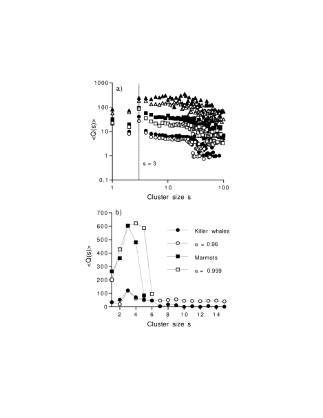
Figure 5: Comparison of numerical predictions with real-world data: a) $\left<Q\left(s\right)\right>$ from agent-based model at $\alpha=0$ (circles), $0.5$ (filled circles), $0.9$ (squares), $0.95$ (filled squares), $0.99$ (triangles) and $0.995$ (filled triangles); b) $\left<Q\left(s\right)\right>$ from killer whales (filled circles) and marmots (filled squares), and corresponding $\left<Q\left(s\right)\right>$ from agent-based model at $\alpha=0.96$ (circles) and $0.99$ (squares).

IV Discussion

We have introduced a model in which interactions between agents are driven by their likelihood to imitate one another. The model supports the formation of spatial clusters that obey the power-law cluster-size frequency distribution over a wide range of possible $\tau$ values. The rules governing allelomimetic interactions are few and simple. A single parameter $\alpha$ ($0\leq\alpha\leq 1$) is needed to tune the exponent $\tau$ value over a wide range of values. Our model is generic and could explain the broad spectrum of $\tau$ values observed with different kinds of real-world scale-free cluster systems (see Table 1).

A nonlinear relation that is described by a Fermi distribution, exists between the degree of allelomimetic behavior (as measured by $\alpha$) and $\tau$ which describes the relative abundance of the cluster sizes in the system. The $\alpha(\tau)$ curve in Fig. 4, accurately tracks the $\tau$ values that have been measured with real-world clusters. Successful correlation between theory and experimental evidence has been achieved even with a simplified agent-based model that neglects possible differences in the allelomimetic behavior among agents. We have assumed that all agents in a given system have the same $\alpha$ and are confined to interact on a two-dimensional plane.

The nonlinear character of the $\alpha(\tau)$ curve indicates the presence of three general classes of allelomimetic interactions namely, blind copying, information-use copying, and non-allelomimetic. Our findings are consistent with previous claims that were derived directly from experimental evidence Wagner and Danchin (2003). Different cluster systems that benefit from blind copying are characterized by a small $\alpha$-range that is near unity. However, such systems yield cluster-size frequency distributions with a wide range of possible $\tau$-values ($0\leq\tau<2$) implying that the relative abundance of the cluster sizes in systems with strongly-allelomimetic agents is sensitive to small variations in $\alpha$. A similar sensitivity characteristic also occurs with non-allelomimetic cluster systems such as colloids and galaxies ($\alpha\approx 0$).

Cluster systems that are formed by humans such as slums, cities, and business firms are associated with a wide range of $\alpha$ values ($0.1\leq\alpha\leq 0.9$). However, their $D\left(s\right)$ plots are restricted within a limited spectrum of $\tau$-values ($1.4\leq\tau<2.16$). Human beings have developed (by evolution and learning from past mistakes) the capability to decide on their own or as a collective based on a set of often contending factors. The formation of slum areas which are anti-social and often illegal entities, is driven by collective action of informal settlers which is a strongly allelomimetic behavior. On the other hand, business firms and the cities in Germany and Japan are formed deliberately based on information-driven plans and project studies. The cluster-size distribution of slum areas tend to be uniform while those of business firms are likely to be biased towards the small and medium sized (in terms of employee number).

In cluster formation that arises from information-use copying, the cluster-size frequency distribution is weakly sensitive to slight $\alpha$ variations ($\alpha\propto\tau$) unlike with the other two classes of allelomimetic behavior. The information-based cluster systems are quite robust – significant shift in the allelomimetic tendency of the component agents only results in a slight change of the cluster-size frequency distribution.

Our model has also predicted that with strongly-allelomimetic agents, the most stable cluster is one with three members ($s=3$). Experimental evidence for this interesting finding has been found in killer whales and marmots. We think that three is a stable company because it is the smallest (hence the most economical to maintain) cluster size where the concept of majority-based decision remains meaningful.

V Conclusions

Allelomimesis (or its absence) is a generic interaction mechanism between adaptive agents that could accurately explain the richness of $\tau$ values that has been observed in real-world scale-free cluster systems. This is possible because allelomimetic interactions between agents can be described by few and simple local rules.

We have generated an $\alpha(\tau)$ curve that rationalizes the broad spectrum of observed $\tau$ values. The curve may be utilized to formulate effective strategies in wildlife conservation, urban planning, and even product marketing. Allelomimesis-based interaction could also explain the existence of a preferred cluster size of $s=3$ in strongly-allelomimetic animals such as killer whales and marmots.

In the real world, it is not unusual to find several cluster systems occupying a common habitat. That each of them can be analyzed with a single model is proof of the underlying interconnectivity of animate and inanimate clusters. The availability of a universal mechanism for adaptation is vital in the formulation of effective strategies in wildlife preservation, environmental management, urban planning, economics, and even politics.

Allelomimesis in endangered species may be enhanced to favor large-cluster formation where reproductive success is greater since survivorship is directly related to group size Parrish and Edelstein-Keshet (1999). Urban overcrowding may be reduced with initiatives that discourage allelomimesis in humans. An efficient army or a successful beauty product may be developed by strategies that favor blind obedience and mass mimicry, respectively.

References

- Bak (1996) P. Bak, How Nature Works - The Science of Self-Organized Criticality (Copernicus, New York, 1996).
- Stanley et al. (1996) H. E. Stanley et al., Physica A 231, 20 (1996).
- Bonabeau and Dagorn (1995) E. Bonabeau and L. Dagorn, Phys. Rev. E 51, R5220 (1995).
- Bonabeau et al. (1999) E. Bonabeau, L. Dagorn, and P. Fréon, Proc. Natl. Acad. Sci. USA 96, 4472 (1999).
- Jarrett (1998) T. Jarrett, 2MASS Galaxy cluster catalog (Infrared Processing and Analysis Center, Jet Propulsion Laboratory, California Insititute of Technology) (1998), available online at, http://www.spider.ipac.caltech.edu/staff/jarrett/2mass/.
- Johansson (1997) D. Johansson, Ph.D. thesis, Stockholm School of Economics, Stockholm, Sweden (1997).
- Axtell (2001) R. Axtell, Science 293, 1818 (2001).
- Huynen and van Nimwegen (1998) M. Huynen and E. van Nimwegen, Mol. Biol. Evol. 15, 583 (1998).
- May (2004) R. May, Science 303, 790 (2004).
- Parrish and Edelstein-Keshet (1999) J. Parrish and L. Edelstein-Keshet, Science 284, 99 (1999).
- Juanico et al. (2003) D. E. Juanico, C. Monterola, and C. Saloma, Physica A 320, 590 (2003).
- Grimm (2003) V. Grimm, Oikos 102, 124 (2003).
- Baird and Dill (1996) R. Baird and L. Dill, Behav. Eco. 7, 408 (1996).
- Wagner and Danchin (2003) R. Wagner and E. Danchin, Anim. Behav. 65, 405 (2003).
- Saloma et al. (2003) C. Saloma et al., Proc. Natl. Acad. Sci. USA 100, 11947 (2003).
- Makse et al. (1995) H. Makse, S. Havlin, and H. E. Stanley, Nature 377, 608 (1995).
- Higgs (2000) P. Higgs, Proc. R. Soc. Lond. B 267, 1355 (2000).
- Milinski et al. (2002) M. Milinski, D. Semmann, and H. J. Krambeck, Nature 415, 424 (2002).
- Armienti and Tarquini (2002) P. Armienti and S. Tarquini, Lithos 65, 273 (2002).
- Ito et al. (2002) Y. Ito, S. Yamane, and K. Tsuchida, J. Ethol. 20, 3 (2002).
- Sjoberg et al. (2000) M. Sjoberg, B. Albrectsen, and J. Hjalten, Ecology Lett. 3, 90 (2000).
- Malamud et al. (1998) B. Malamud, G. Morein, and D. Turcotte, Science 281, 1840 (1998).
- Perkins and Edwards (1997) P. Perkins and E. Edwards, Administrative Report LJ-97-03, Southwest Fisheries Center, La Jolla, California (1997).
- Altmann and Altmann (1970) S. Altmann and J. Altmann, Baboon ecology, African field research (Univ. of Chicago Press, Chicago, 1970).
- Kadel et al. (1991) J. Kadel, A. Dukeman, and G. Patton, Technical Report 228, Natural Resources Department, County of Sarasota (1991).
- Schaller (1972) G. B. Schaller, The Serengeti lion, a study of predator-prey relations (Univ. of Chicago Press, Chicago, 1972).
- Sobreira and Gomes (2001) F. Sobreira and M. Gomes, Working Paper 30, Centre for Advanced Spatial Analysis, University College London, UK (2001).
- van Ark and Monnikhof (1996) B. van Ark and E. Monnikhof, Working Paper 166, Economics Dept., Organisation for Economic Cooperation and Development, University College London, UK (1996).
- Brinkhoff (2004) T. Brinkhoff, City population: Principal cities and agglomerations of the world (2004), available online at, http://www.citypopulation.de.
- Simon and Bonini (1958) H. Simon and C. Bonini, Am. Econ. Rev. 48, 607 (1958).
- Domb (1973) C. Domb, Phase Transitions and Critical Phenomena (Academic Press, New York, 1973), vol. 8.
- Hoshen and Kopelman (1976) J. Hoshen and R. Kopelman, Phys. Rev. B 14, 3438 (1976).
- Burroughs and Tebbens (2001) S. Burroughs and S. Tebbens, Pure Appl. Geophys. 158, 741 (2001).
- Bauer (1988) W. Bauer, Phys. Rev. C 38, 1297 (1988).
- Culik (2003) B. Culik, Orcinus orca, Killer whale (2003), available online at, http://www.wcmc.org.uk.
- Armitage and Schwartz (2000) K. Armitage and O. Schwartz, Proc. Natl. Acad. Sci. USA 97, 12149 (2000).
- Smith (2001) S. Smith, The biogeography of the yellow-bellied marmot (San Francisco State Univ., Dept. of Geography) (2001), available online at, http://bss.sfsu.edu.224/courses/.