The effect of noise on the dynamics of a complex map at the period-tripling accumulation point

Abstract

As shown recently (O.B.Isaeva et al., Phys.Rev E64, 055201), the phenomena intrinsic to dynamics of complex analytic maps under appropriate conditions may occur in physical systems. We study scaling regularities associated with the effect of additive noise upon the period-tripling bifurcation cascade generalizing the renormalization group approach of Crutchfield et al. (Phys.Rev.Lett., 46, 933) and Shraiman et al. (Phys.Rev.Lett., 46, 935), originally developed for the period doubling transition to chaos in the presence of noise. The universal constant determining the rescaling rule for the intensity of the noise in period-tripling is found to be $\gamma=12.2066409...$ Numerical evidence of the expected scaling is demonstrated.

PACS numbers: 05.45.-a, 05.45.Df, 05.10.Cc, 05.40.Ca

Institute of Radio-Engineering and Electronics of RAS, Saratov Branch,
Zelenaya 38, Saratov, 410019, Russia

Department of Mathematics, University of Portsmouth,
Portsmouth, PO1 3HE, UK

1 INTRODUCTION

Application of the renormalization group (RG) analysis and the concepts of universality and scaling in nonlinear dynamics started with the works of Feigenbaum concerning the period-doubling transition to chaos [1]. The universal quantitative regularities intrinsic to this type of behavior are common for a wide class of systems including one-dimensional maps, forced dissipative nonlinear oscillators, Rössler and Lorenz models, experimental systems in hydrodynamics, electronics, laser physics, etc [2]. In the context of real systems, a question of vital importance is the effect of noise on the dynamics at the onset of chaos. It is more or less obvious that the presence of noise destroys subtle details of the small-scale (or long-time) dynamics. The RG analysis developed by Crutchfield et al. [3] and by Shraiman et al.  [4] gives a quantitative measure for this effect. Namely, to observe one more level of period doubling it is needed to decrease the noise amplitude by the factor $\gamma=6.61903$.

After Feigenbaum the RG approach was developed by many authors, e.g. for the onset of chaos via quasiperiodicity and intermittency [5, 6], as well as for some situations arising in the multiparameter analysis of transition to chaos [7] or to strange nonchaotic attractors [8]. In particular, the effects of noise on the dynamics have been studied in dissipative systems for intermittency [9], quasiperiodicity [10], bicritical behavior [11], and in Hamiltonian systems for period doubling [12] and KAM-torus destruction [13].

A special kind of dynamics occurs in iterative complex analytic maps $z_{n+1}=f(z_{n})$ [14]. An example is a complex quadratic map

$$z_{n+1}=\lambda-z_{n}^{2},$$ (1)

which gives rise to remarkable fractal formations in the complex plane of the variable $z$ (the Julia sets) and of the complex parameter $\lambda$ (the Mandelbrot set). The latter is defined by the condition that being launched from the origin, the iterations at a given $\lambda$ never diverge. The Mandelbrot set has a subtle and complicated structure, which is a subject of extensive research. In particular, it contains special points of accumulation of bifurcation cascades. Beside the period doubling, there are also cascades of period tripling, quadrupling, etc. The period-tripling accumulation point has been studied first by Golberg, Sinai, and Khanin [15] (see also [16]), and will be referred to as the GSK critical point . In the map (1) it is located at

$$\lambda_{c}=0.0236411685377+0.7836606508052i.$$ (2)

By analogy with Feigenbaum universality, it could be expected to occur in other nonlinear systems as well.

However, in fact, complex analytic functions represent a very special and restricted class of maps because real and imaginary parts of $f(z)$ must satisfy the Cauchy-Riemann equations. If this is not the case, the dynamics become drastically different [17]. In particular, it was shown that the period-tripling type of behavior does not survive, in general, under a non-analytic perturbation [18] (in spite of the claim in the original paper [15] and some other works [19, 20]). So, a principal question is: Do the phenomena intrinsic to complex analytic maps have any concern to dynamical behavior of physical systems? One example of an appropriate physical system was suggested by Beck [21]. Another approach developed in Ref. [22] is based on a construction of a system of two coupled units, each of which can demonstrate Feigenbaum’s period-doubling cascade, and the coupling is of some special kind. Moreover, this idea has been verified in an experiment with coupled electronic circuits.

Recognizing a possibility of the physical occurrence of the phenomena of complex analytic dynamics, we intend to study in this paper the effect of noise on the period-tripling cascade in the spirit of the earlier works of Crutchfield et al.  [3] and Shraiman et al.  [4], on a basis of the appropriate generalization of the RG approach.

2 RENORMALIZATION GROUP ANALYSIS

If we perform $3^{k}$ iterations of the map (1) at the GSK critical point $\lambda=\lambda_{c}$, the renormalized evolution operator will converge, as known, to a universal function

$$\lim\limits_{k\rightarrow\infty}f^{3k}(zf^{3k}(0))/f^{3k}(0)=g(z),$$ (3)

which satisfies the fixed-point RG equation

$$g(z)=\alpha g(g(g(z/\alpha))).$$ (4)

Obviously, $g(z)$ represents an evolution operator at the critical point for an asymptotically large number of iterations $3^{k}$ in terms of the properly normalized dynamical variable. Numerically, the approximation for this function was found in Ref. [15] as a finite Taylor series:

$$g(z)\cong 1+(0.0547-0.7490i)z^{2}+(-0.0244-0.0525i)z^{4}+...$$ (5)

together with the complex scaling constant

$$\alpha=1/g(g(g(0)))\cong-2.09691989+2.35827964i.$$ (6)

Let us introduce noise and consider a stochastic equation

$$z_{n+1}=g(z_{n})+\varepsilon\varphi(z_{n})\xi_{n},$$ (7)

where $\varepsilon$ is a small parameter of the noise intensity, $\varphi(z)$ is a smooth real function of complex argument, and $\xi_{n}$ is a complex stationary random sequence with statistically independent subsequent terms. We assume that it has zero mean, unit mean square $\langle|\xi_{n}^{2}|\rangle=1$, and zero correlation of the real and imaginary parts, $\langle(\mathrm{Re}\xi_{n})(\mathrm{Im}\xi_{n})\rangle=0$. It is expected that the scaling properties of the response under study will be independent on the concrete form of the distribution function, although it is convenient to suppose that a distribution function for $\xi_{n}$ is of such kind that the amplitude of the noise is bounded.

Three-fold application of the stochastic map yields, in the first order in $\varepsilon$,

$$\begin{array}[]{l}z_{n+3}=g(g(g(z_{n})))+\varepsilon\{g^{\prime}(g(g(z_{n})))g^{\prime}(g(z_{n}))\varphi(z_{n})\xi_{n}\\ +g^{\prime}(g(g(z_{n})))\varphi(g(z_{n}))\xi_{n+1}+\varphi(g(g(z_{n})))\xi_{n+2}\}.\end{array}$$ (8)

Now, we renormalize the variable $z$ by substitution $z\rightarrow z/\alpha$, and obtain

$$\begin{array}[]{l}z_{n+3}=\alpha g(g(g(z_{n}/\alpha)))+\varepsilon\alpha\{g^{\prime}(g(g(z_{n}/\alpha)))g^{\prime}(g(z_{n}/\alpha))\varphi(z_{n}/\alpha)\xi_{n}\\ +g^{\prime}(g(g(z_{n}/\alpha)))\varphi(g(z_{n}/\alpha))\xi_{n+1}+\varphi(g(g(z_{n}/\alpha)))\xi_{n+2}\}.\end{array}$$ (9)

The first term in the right-hand part of the equation equals $g(z)$, in accordance with Eq. (4). Concerning the remaining terms, we make the following important remark. Let us suppose that we start at some $z_{n}.$ Consider an ensemble of the random numbers $\{\xi_{n},\xi_{n+1},\xi_{n+2}\}$ and compose them with complex coefficients given by functions of $z_{n}.$ As $\{\xi_{n},\xi_{n+1},\xi_{n+2}\}$ are independent, the sum can be represented again as a random complex number with zero mean and unit mean square multiplied by a real function of complex argument, namely,

$$\begin{array}[]{l}\alpha\{g^{\prime}(g(g(z_{n}/\alpha)))g^{\prime}(g(z_{n}/\alpha))\varphi(z_{n}/\alpha)\xi_{n}\\ \qquad\quad\quad+g^{\prime}(g(g(z_{n}/\alpha)))\varphi(g(z_{n}/\alpha))\xi_{n+1}+\varphi(g(g(z_{n}/\alpha)))\xi_{n+2}\}=\hat{\varphi}(z_{n})\hat{\xi}_{n}.\end{array}$$ (10)

So, we rewrite (9) in the form analogous to (7), with redefined function and random variable in the stochastic term:

$$z_{n+3}=g(z_{n})+\varepsilon\hat{\varphi}(z_{n})\hat{\xi}_{n}.$$ (11)

To obtain a closed functional equation, we multiply both parts of Eq. (10) by the complex conjugates, and perform an averaging over an ensemble of realizations of the noise. As $\langle|\hat{\xi}^{2}_{n}|\rangle=\langle|\xi^{2}_{n}|\rangle=1$, and $\langle\xi_{n}\xi^{*}_{n+1}\rangle=\langle\xi_{n}\xi^{*}_{n+2}\rangle=0$, we come to the relation

$$\begin{array}[]{l}\hat{\Phi}(z_{n})=|\alpha|^{2}\{|g^{\prime}(g(g(z_{n}/\alpha)))g^{\prime}(g(z_{n}/\alpha))|^{2}\Phi(z_{n}/\alpha)+|g^{\prime}(g(g(z_{n}/\alpha)))|^{2}\Phi(g(z_{n}/\alpha))+\Phi(g(g(z_{n}/\alpha)))\},\end{array}$$ (12)

where $\Phi(z)=[\varphi(z)]^{2}$. Obviously, Eq. (12) has a structure $\hat{\Phi}(z)=\mathbf{L}\Phi(z)$, where $\mathbf{L}$ is a linear operator of the functional transformation given by the right-hand part of (12). Repetitive application of the same procedure to Eq. (11) yields a sequence of functions with asymptotic behavior $\Phi_{k}(z)\cong\Omega^{k}\Phi(z)$, determined by eigenvector $\Phi(z)$, associated with the largest eigenvalue $\Omega$ of the operator $\mathbf{L}$:

$$\begin{array}[]{l}\Omega\Phi(z)=|\alpha|^{2}\{|g^{\prime}(g(g(z/\alpha)))g^{\prime}(g(z/\alpha))|^{2}\Phi(z/\alpha)+|g^{\prime}(g(g(z/\alpha)))|^{2}\Phi(g(z/\alpha))+\Phi(g(g(z/\alpha)))\}.\end{array}$$ (13)

As mentioned above, the universal function $g(z)$ has been approximated as a finite expansion over even powers of the argument [15]. Using this data, we have numerically constructed the functional transformation of the right-hand part of Eq (13). The unknown function $\Phi(z)$ is represented by a set of real values at nodes of a grid in a square $\{-1.2<\mathrm{Re}z,\mathrm{Im}z<1.2\}$, and by an interpolation scheme between them. Taking random initial conditions for $\Phi(z)$, we perform the functional transformation and normalize the resulting function as $\Phi^{0}(z)=\Phi(z)/\Phi(0)$. This operation is repeated many times, until the form of the function stabilizes (see Fig. 1). The value of $\Phi(0)$. (before the normalization) converges to the eigenvalue $\Omega=149.0020828$.

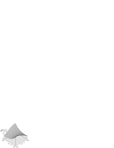
Figure 1: Plot of the eigenfunction responsible for the effect of noise at the period tripling accumulation point obtained numerically (see text).

In the linear approximation with respect to the noise amplitude, the stochastic map for the evolution over $3^{k}$ steps at the GSK critical point asymptotically may be written as

$$z_{n+3^{k}}=g(z_{n})+\varepsilon\gamma^{k}\varphi(z_{n})\xi_{n},$$ (14)

where

$$\varphi(z)=\sqrt{\Phi^{0}(z)},\quad\gamma=\sqrt{\Omega}=12.20664093.$$ (15)

If we consider a small shift of $\lambda$ from the GSK critical point, then an additional perturbation term appears in the equation:

$$z_{n+3^{k}}=g(z_{n})+C_{1}\delta_{1}^{k}h_{1}(z_{n})+\varepsilon\gamma^{k}\varphi(z_{n})\xi_{n}.$$ (16)

Here, $h_{1}(z)$ represents an eigenvector of the linearized RG equation without noise associated with the eigenvalue $\delta_{1}=4.60022558-8.98122473i$. The coefficient $C_{1}$ depends on the parameter and vanishes at the critical point GSK. In a close neighborhood of the critical point it is sufficient to consider only the leading terms of the expansion and set $C_{1}\propto(\lambda-\lambda_{c})$.

Now, we are ready to formulate the basic scaling property that follows from (16).

If we triple the number of time steps (i.e., change $k$ to $k+1$), decrease the parameter difference $\Delta\lambda=\lambda-\lambda_{c}$ by division by $\delta_{1}$, and decrease noise amplitude $\varepsilon$ by factor $\gamma$, then the form of the stochastic map (16) remains unchanged. Thus, with the new parameters, ($\Delta\lambda/\delta_{1}$, $\varepsilon/\gamma$) the noisy system will demonstrate the same behavior as that with the old ones, but with a tripled time scale.

3 MODEL MAP AND NUMERICAL EXPERIMENTS

To verify the RG results in numerical experiments, we use a model map with additive noise:

$$z_{n+1}=\lambda-z_{n}^{2}+\varepsilon\xi_{n}.$$ (17)

Real and imaginary parts for each term of the complex random sequence $\xi_{n}$, are obtained as sums of $N=10$ zero-mean computer generated pseudo-random numbers, which are properly normalized to have $\langle|\xi_{n}^{2}|\rangle=1$. (In accordance with the central limit theorem, $\xi_{n}$ is very close to a Gaussian random variable.)

Fig. 2 illustrates fine structure of the Mandelbrot set near the period-tripling accumulation point as it looks (a) in the absence and (b) in the presence of noise. The pictures represent the Lyapunov charts for the complex parameter $\lambda$. (See [23, 18] for previous applications of this method.) At each pixel of the two-dimensional plot we estimate the Lyapunov exponent

$$\Lambda=\lim\limits_{N\rightarrow\infty}N^{-1}\sum\limits_{n=1}^{N}\ln|2z_{n}|$$ (18)

from numerical computations, and mark the pixel with a gray tone. The tones vary from dark to light as the Lyapunov exponent varies from large negative to zero: white corresponds to zero, and black to positive Lyapunov exponent. Divergence is shown by uniform coloring with one special gray tone. The GSK critical point is located exactly at the center of the diagram. A small box containing the critical point, is magnified and rotated in accordance with multiplication by $\delta_{1}\approx 4.6002-8.9812i$. As the parameter rescaling is associated with a tripling of characteristic time scale, we accompany it with reducing an interval for gray coding of Lyapunov exponents by factor $1/3$ for each successive picture in the row. On the panel (a) such diagrams are shown for zero amplitude of noise, $\varepsilon=0$, and on panel (b) for noise of fixed intensity, $\varepsilon=0.001$. Observe the similarity of the leaves of the ”Mandelbrot cactus” in the first case, and the progressive destruction of the structure at subsequent levels of the resolution in the second.

In Fig. 3

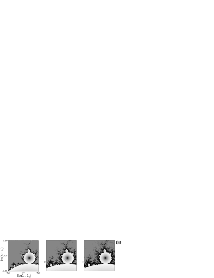
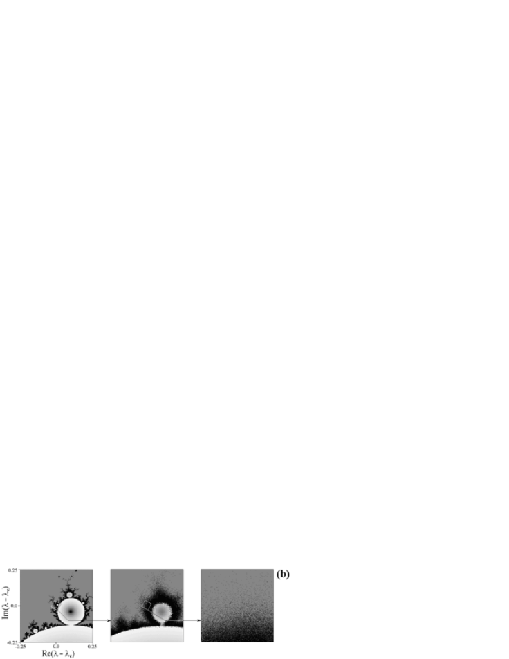
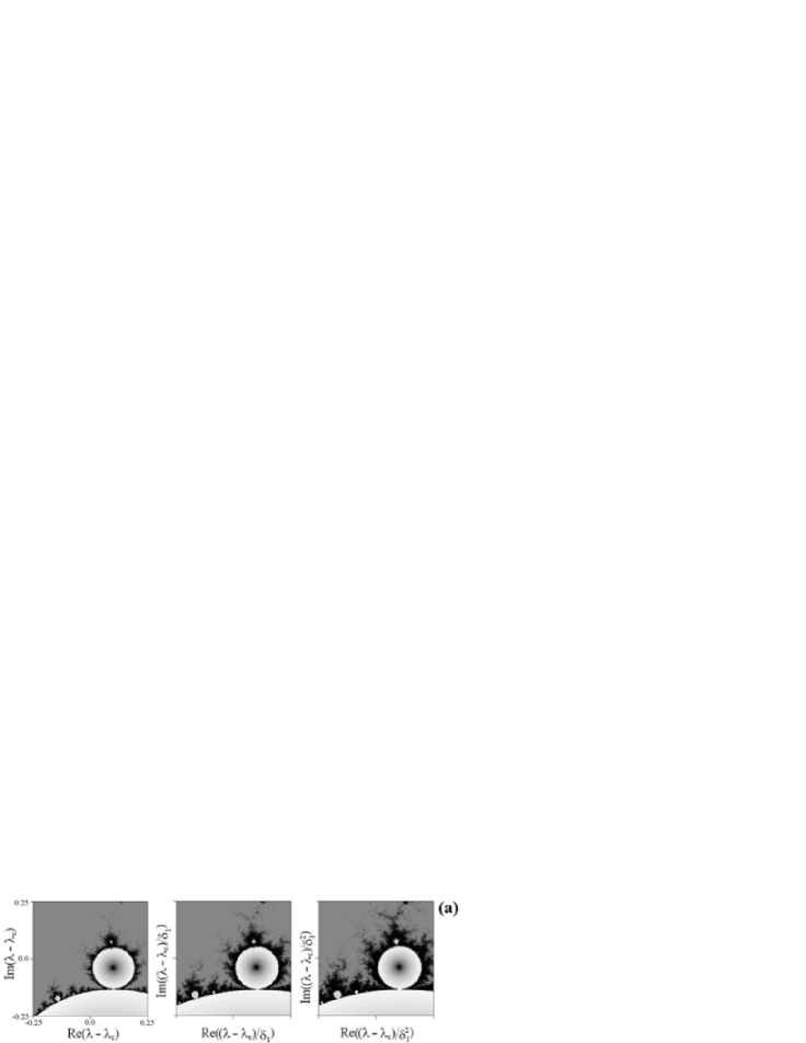
Figure 2: The Lyapunov charts for the model map (17) on the complex parameter plane for zero intensity of noise $\varepsilon=0$ (a) and in presence of noise, $\varepsilon=0.001$ (b). The GSK critical point is located exactly at the center of the diagrams. The tones vary from dark to light as the Lyapunov exponent varies from large negative to zero: white corresponds to zero, and black to positive values. Divergence is shown by uniform coloring with one special gray tone. A small box containing the critical point, is magnified and rotated in accordance with multiplication by $\delta_{1}\approx 4.6002-8.9812i$. The interval for coded values of Lyapunov exponents is reduced with factor $1/3$ for each successive picture in the row to visualize self-similarity of the pictures in absence of noise.

Figure 3: Lyapunov charts for the stochastic model (17) on the complex parameter plane in presence of noise for $\varepsilon=\varepsilon_{1}=0.003$, $\varepsilon=\varepsilon_{1}/\gamma$, and $\varepsilon=\varepsilon_{1}/\gamma^{2}$ (a), and for $\varepsilon=\varepsilon_{2}=0.009$, $\varepsilon=\varepsilon_{2}/\gamma$, and $\varepsilon=\varepsilon_{2}/\gamma^{2}$ (b). The GSK critical point is located exactly at the center of the diagrams. The coordinate rescaling rule and the gray coding are the same as in Fig. 2. The interval for coded values of Lyapunov exponents is reduced with factor $1/3$ for each succesive picture in the row to visualize the similarity of the pictures.

we show analogous pictures with noise, but now its intensity is reduced for each subsequent picture in a row by the factor $\gamma=12.2066...$ found from the RG analysis. Panels (a) and (b) correspond to different initial levels of the noise, respectively, $\varepsilon=0.003$ and $0.009$. Now, the similarity of the pictures is restored. With noise reduction by $\gamma$, just one more level of smaller leaves of the Mandelbrot cactus reveals itself near the GSK critical point.

Fig. 4

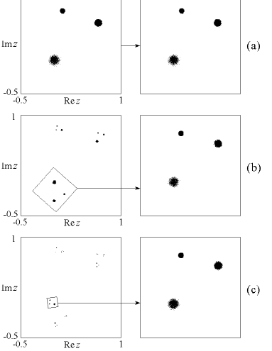
Figure 4: Similarity in structure of the noisy attractors for the model map (17) on the plane of complex variable $z$. The parameter $\lambda$ values are $0.122561167+0.744861767i$ (a), $0.031552975+0.790783175i$ (b), $0.023369416+0.784679678i$ (c), and the noise intensities are $\varepsilon=0.015$, $0.015/\gamma$, and $0.015/\gamma^{2}$, respectively, where $\gamma=12.2066$ The right-hand pictures represent the definite parts of the attractors drawn with rescaling by complex factors $\alpha=-2.0959...+i2.3582...$ (b) and $\alpha^{2}$ (c).

illustrates similarity in structure of the noisy attractors for the model map (17) in the plane of the complex variable $z$. Diagrams (b) and (c) relate to noise intensities reduced by the factors $\gamma$ and $\gamma^{2}$ in comparison with the plot (a). The parameter $\lambda$ values correspond to the superstable cycles of period $3$, $9$, and $27$, respectively. The right-hand panels show the indicated parts of the pictures drawn with rescaling by complex factors $\alpha$ (diagram (b)) and $\alpha^{2}$ (diagram (c)). Observe the similarity of the right-hand diagrams.

4 CONCLUSION

In this paper we have studied the effect of noise on a complex analytic map at the period-tripling accumulation point. It was shown that the effect of noise obeys regularities of a similar nature to those reported for period doubling in real one-dimensional maps. Namely, to observe one more level of the bifurcation cascade it is needed to decrease the intensity of noise by some definite scaling factor. For the case of the period-tripling this factor has been found to be $12.2066...$, as follows from the renormalization group analysis. Also we have demonstrated the scaling properties associated with the new constant in numerical experiments.

The undertaken analysis is essential for discussion of the possibility of observation of phenomena of complex analytic dynamics in real physical experiment, e.g. in mechanics or electronics [21, 22, 18]. The presence of noise in such systems is inevitable, and our result gives a quantitative foundation for estimates of an observable number of levels in the bifurcation cascade.

Our work puts the phenomena in complex analytic map into the same context in respect to the effect of noise, as other situations of universal scaling behavior: period doubling [3, 4], intermittency [9], quasiperiodicity [10], bicriticality [11], scaling phenomena in Hamiltonian systems [12, 13]. So, this specific field is enriched with one more nontrivial example of the scaling behavior linked with presence of noise.

The approach developed in this article may be adapted to study the effect of noise on other bifurcation cascades in complex analytic maps (”$n$-tupling” with $n=4,5,...$ [13, 16]). Moreover, it gives a basis from which to pose more general questions on the effect of noise on the Mandelbrot-like sets in physical systems possessing such kind of objects in their parameter space.

References

- [1] M. J. Feigenbaum, J. Stat. Phys. 19, 25 (1978); M.J. Feigenbaum, J. Stat. Phys. 21, 669 (1979); M.J. Feigenbaum, Physica D 7, 16 (1983).
- [2] P. Cvitanović, ed. Universality in Chaos(Adam Hilger, 2nd Edition, 1989).
- [3] J.P. Crutchfield, M. Nauenberg, J. Rudnik, Phys. Rev. Lett. 46, 933 (1981).
- [4] B. Shraiman, C. E. Wayne, P. C. Martin, Phys. Rev. Lett. 46, 935 (1981).
- [5] B. Hu, J. Rudnik, Phys. Rev. Lett. 48, 1645 (1982).
- [6] S. J. Shenker, Physica D 5, 405 (1982); M. J. Feigenbaum, L. P. Kadanoff, S.J. Shenker, Physica D 5, 370 (1982); D. Rand, S. Ostlund, J. Sethna, E. D. Siggia, Phys. Rev. Lett. 49, 132 (1982).
- [7] A. P. Kuznetsov, S. P. Kuznetsov, I. R. Sataev, Physica D 109, 91 (1997).
- [8] S. P. Kunetsov, A. S. Pikovsky and U. Feudel, Phys. Rev. E 51, R1629 (1995); S. P. Kuznetsov, U. Feudel and A. S. Pikovsky, Phys. Rev. E 57, 1585 (1998); S. P. Kuznetsov, E. Neumann, A. Pikovsky, I. R. Sataev, Phys. Rev. E 62, 1995 (2000); S. P. Kuznetsov, Phys. Rev. E 65, 066209 (2002).
- [9] J. E. Hirsch, B. A. Huberman, D. J. Scalapino, Phys. Rev. A 25, 519 (1981); J. E. Hirsch, M. Nauenberg, D. J. Scalapino, Phys. Lett. A 87, 391 (1982); J. P. Eckmann, L. Thomas, P. Wittwer, J. Phys. A 14, (1981).
- [10] A. Hamm and R. Graham, Phys. Rev. A 46, 6323 (1992).
- [11] J. V. Kapustina, A. P. Kuznetsov, S. P. Kuznetsov, and E. Mosekilde, Phys. Rev. E 64, 066207 (2001).
- [12] G. Gyorgyi and N. Tishby, Phys. Rev. Lett. 58, 527 (1987).
- [13] G. Gyorgyi and N. Tishby, Phys. Rev. Lett. 62, 353 (1989).
- [14] H.-O. Peitgen, P. H. Richter, The beauty of fractals. Images of complex dynamical systems(Springer-Verlag, 1986); R.L. Devaney, An Introduction to Chaotic Dynamical Systems(Addison-Wesley Publ, 1989).
- [15] A.I. Golberg, Y. G. Sinai, K. M. Khanin, Russ. Math. Surv. 38, 187 (1983).
- [16] P. Cvitanovic, J. Myrheim, Phys. Lett. A 94, 329 (1983); P. Cvitanovic, J. Myrheim, Commun. Math. Phys. 121, 225 (1989).
- [17] J. Peinke, J. Parisi, B. Rohricht, and O. E. Rossler, Zeitsch. Naturforsch. A 42, 263 (1987); M. Klein, Zeitsch. Naturforsch. A 43, 819 (1988); B.B. Peckham, Int. J. of Bifurcation and Chaos 8, 73 (1998); B.B. Peckham, Int. J. of Bifurcation and Chaos 10, 391 (2000).
- [18] O. B. Isaeva, S. P. Kuznetsov, Regular and Chaotic Dynamics 5, 459 (2000).
- [19] G. H. Gunaratne, Phys. Rev. A 36, 1834 (1987).
- [20] V. I. Arnold (ed.), Dynamical Systems V: Bifurcation Theory and Catastrophe Theory(Berlin, Heidelberg, New York, London, Springer Verlag, 1994).
- [21] C. Beck, Physica D 125, 171 (1999).
- [22] O. B. Isaeva, S. P. Kuznetsov, V. I. Ponomarenko, Phys. Rev E 64, 055201 (2001).
- [23] J. Rossler, M. Kiwi, B. Hess, and M. Markus, Phys. Rev. A 39, 5954 (1989); M. Marcus, B. Hess, Computers & Graphics 13, 553 (1989); A.P. Kuznetsov, A.V. Savin, Nonlinear Phenomena in Complex Systems 5, 296 (2002).