Drag Reduction by Microbubbles in Turbulent Flows: the Limit of Minute Bubbles
Abstract
Drag reduction by microbubbles is a promising engineering method for improving ship performance. A fundamental theory of the phenomenon is lacking however, making actual design quite up-hazard. We offer here a theory of drag reduction by microbubbles in the limit of very small bubbles, when the effect of the bubbles is mainly to normalize the density and the viscosity of the carrier fluid. The theory culminates with a prediction of the degree of drag reduction given the concentration profile of the bubbles. Comparisons with experiments are discussed and the road ahead is sketched.
pacs:
47.27.Rc, 47.55.Dz, 83.60.YzThe idea of reducing drag friction by placing a thin layer of air between a ship and its water boundary was patented already in the nineteenth century patent . Drag reduction by the injection of microbubbles into the turbulent boundary layer has been the subject of intensive research since the first experimental observation of this phenomenon in 73BM , and see the comprehensive review 90MD . The reduction of skin-friction drag by microbubbles has important technological and engineering advantages, especially for marine transportation by huge and relatively slow ships like tankers, but also for many other applications, such as hydro-foils, in-pipe transportation, etc. The voluminous literature on the engineering aspects of the problem cannot be referenced in full. It suffices to mention impressive results such as the microbubble drag reduction by about 80% on a flat plane, 85MDM , and up to 32% on a 50 m long flat plane ship, see 99TKMYK . Some steps in understanding the phenomenon have been made. Ref 77BEM found that the drag reduction correlates with the maximum void fraction in the boundary layer. It was understood that the “local distribution and shape [of the microbubble void fraction ] in the boundary layer have paramount influence in the drag reduction” 02HV . Many researches (see, e.g. 98Wat ) found that effect of micro-bubbles decreases downstream and that the bubble size is another important factor influencing frictional resistance.
Legner 84Leg stated that the “decrease of the medium density as the gas concentration increases provides the primary drag reduction mechanism”. Unfortunately, the analysis of Ref. 84Leg does not contain any spatial dependencies, taking the distribution of bubble void fraction to be homogeneous. In addition Legner 84Leg concluded that the increase of the dynamic fluid viscosity, caused by the bubbles, leads to increase of frictional drag. In contradiction, other studies (see, e.g. Ref. 99Kat ) lead to the opposite conclusion: that the increase of the viscosity, caused by microbubbles, decreases the friction drag. To date this confusion has not been resolved theoretically.
The aim of this Letter is to offer a theory of drag reduction by microbubbles in the limit that their diameter is very small (), and the void fraction is fixed, and not too large (). In addition we will assume that the scale of variation where is the distance from the wall. The advantage of a theory in this limit is that we can show quite rigorously that the only mechanism for drag reduction available in this limit is provided by the reduction of the fluid density and the increase in the fluid viscosity. This is not to say that there are no additional possible mechanisms of drag reduction by microbubbles due to their influence on the structure of turbulence, including near wall coherent structures 02MK ; 04FE ; 04SKTM . The theoretical description of such effects is however very difficult; they stem entirely from finite bubble-size effects, and they should be taken only as a further step in the development of the theory.
As a starting point for the theoretical development we take the two-fluid description of turbulent flows with bubbles which is presented in Ref. 97ZP . In this description the bubbles are of diameter which is very small. We do not consider individual bubbles, but rather describe them by a field of void fraction and velocity . The carrier fluid has density , viscosity and velocity . We will take the air density of the bubbles to be zero and the acceleration due to gravity, , to act in the direction which is normal to the wall. Disregarding terms of the order of one write the equation of motion
| (1) | |||
| (2) |
In these equations
The effective viscosity which appears in these equations is determined by the bubble concentration,
| (3) |
These equation should be supplemented with the continuity equations
| (4) | |||||
| (5) |
We now simplify the equations further in the limit by evaluating the term proportional to in Eq. (1) using the same term in Eq. (2). We find
| (6) | |||||
In the same limit and .
After some further simplifications in which we retain only terms linear in one gets:
| (7) | |||||
| (8) |
where the effective density of the suspension is
| (9) |
The important conclusion is that dilute () solutions of minute microbubbles () can be described by a one-fluid model with modified density and viscosity . Note that velocity field remains incompressible; this result is valid for minute microbubbles for arbitrary concentrations . Having these results at hand we are poised to offer a theory of drag reduction that is quite similar to the theory by the same authors for drag reduction by flexible polymers 04LPPT .
Consider a flow in channel geometry (with half channel width ); the mean flow is in the direction, the wall normal direction is and the span-wise direction is . We take the bubble concentration to be given and time independent. The fluid velocity is a sum of its average (over time) and a fluctuating part:
| (10) |
For channel flows all the averages, and in particular , are functions of only. The objects that enter the theory are the mean shear , the Reynolds stress and the kinetic energy ; these are defined respectively as
Under the assumption we derive point-wise balance equation for the flux of mechanical momentum, relating these objects 04LPPT ; 04LPT . Near the wall it reads:
| (11) |
On the RHS of this equation we see the production of momentum due to the pressure gradient; on the LHS we have the Reynolds stress and the viscous contribution to the momentum flux, with the latter being usually negligible (in Newtonian turbulence ) everywhere except in the viscous boundary layer.
A second relation between , and is obtained from the energy balance. The energy is created by the large scale motions at a rate of . It is cascaded down the scales by a flux of energy, and is finally dissipated at a rate , where . We cannot calculate exactly, but we can estimate it rather well at a point away from the wall. When viscous effects are dominant, this term is estimated as (the velocity is then rather smooth, the gradient exists and can be estimated by the typical velocity at over the distance from the wall). Here is a constant of the order of unity. When the Reynolds number is large, the viscous dissipation is the same as the turbulent energy flux down the scales, which can be estimated as where is the typical eddy turn over time at . The latter is estimated as where is another constant. We can thus write the energy balance equation at point as
| (12) |
where the bigger of the two terms on the LHS should win. We note that contrary to Eq. (11) which is exact, Eq.(12) is not exact. It was shown however to give excellent order of magnitude estimates as far as drag reduction is concerned 04LPPT ; 04BLPT . Finally, we quote the experimental fact pope ; 01PNVH that outside the viscous boundary layer
| (13) |
with the coefficient rigorously bounded from above by unity (The proof is , because ).
We can change variables now in favor of wall units according to
In these units our balance equations read
| (14) | |||
| (15) |
This set of equations is readily solved, giving
| (16) | |||
| (17) |
In these equations we defined , . The mean velocity anywhere in the channel can be obtained by integrating,
| (18) |
A measure of drag reduction is the relative increase in the mean centerline velocity in the bubbly flow with respect to the neat Newtonian fluid:
| (19) |
Clearly, corresponds to the drag reduction, while to the drag enhancement. We obtain an expression for from Eq. (18) by expanding to linear order in (where our equations are valid anyway):
| (20) |
Here the response function consist of two parts, one due to the density variation and the other due to the viscosity variation :
| (21) | |||||
| (22) | |||||
| (23) |
In writing Eq. (20) we have used the fact that in experiments the bubbles tend to be localized in a finite region near the wall, i.e. sufficiently fast as , and we extended the integration range to infinity.
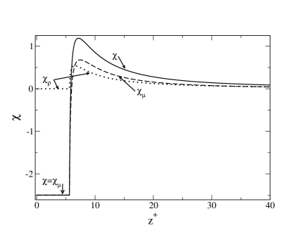
Eqs. (20)-(23) are the main theoretical predictions of this Letter. To complement the theory we present now estimates of the numerical value of the expected drag reduction, and compare it with a relevant experiment. The simplest model takes the parameters in Eq. (LABEL:params) as -independent, and in agreement with the classical von Kármán boundary layer theory, i.e. and . Evaluating the response function with these parameters results with the findings presented in Fig. 1. We see that in the viscous layer, where Eq. (16) is relevant, while is negative. This means that having a bubble concentration in this region does not buy us drag reduction due to the density variation, but it leads to drag enhancement due to the viscosity increase. This is far from being surprising, since in this region the momentum flux is dominated by the viscous term . For a fixed momentum flux any increase in viscosity must decrease and correspondingly lead to drag enhancement. The most efficient drag reduction can be obtained by placing the bubble concentration out of the viscous layer, but not too far from the wall, say at . In this region both the decrease in density and the increase in viscosity lead to drag reduction. The momentum in this region is transported mainly by the Reynolds stress . The effect of density reduction is absolutely clear: it leads to the reduction in momentum flux. For a given momentum generation this has to result in the increase of the mean momentum of the flow. More interesting and counter-intuitive is the effect of increasing viscosity. In order to understand it, we remind the reader that for intermediate values of there is no well-developed turbulent cascade, and outer and inner scales of turbulence are of the same order of magnitude. Therefore the increase of viscosity reduces the turbulent energy, in contrast to fully developed turbulence where changes of viscosity simply modify the Kolmogorov scale without any effect on the turbulent energy, that is dominated by the outer scale. The decrease in turbulent energy here reduces the Reynolds stress, see Eq. (13). It is interesting to note that this effect of increasing viscosity is essentially the same as the mechanism for drag reduction in the case of elastic polymers 04LPPT ; 04BLPT . For polymers, however, the increase in viscosity can be very significant and the linear approximation that is used here is not applicable.
In comparing with experiments we need to consider low bubble concentrations. An interesting experiment was reported in 99Kat , where both and the are shown. We note that this experiment deals with a developing boundary layer rather than a steady channel geometry, but near the wall the Reynolds number can be considered rather time-independent. Digitizing the published profiles and integrating them numerically against our function we obtain results for which appear in good agreement with the data of 99Kat , as long as is small, . For the two lowest values of bubble concentration we agree with the data to within 10-20%, which is definitely within the experimental error bars. For higher values of the results of the experiment become sensitive to nonlinear effects.
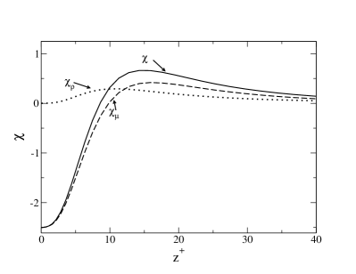
It appears extremely worthwhile to test the theory presented here by numerical simulations that would be designed to do so. We should stress that a careful measurement of in either experiments or simulations, in addition to a determination of , can provide a very good test of our theory. Eq. (20) is more general than our model (17), and it can be tested directly if and its derivative are known. Since the response function is a property of the reference (Newtonian) flow, we can take it from Newtonian data. As an example of such a calculation we have considered the results of numerical simulations for a Newtonian channel flow available in 99MKM , where the profile is provided. We have used it to compute the response function and its two contributions according to Eqs. (21)-(22). The results are presented in Fig. 2. We see that the qualitative predictions of our model for are excellently reproduced by the numerical data, even though the smoother cross over between the viscous and logarithmic layers translates to smoother functions and . A similar comparison for channel flow with bubbles will shed important additional light on our approach.
We reiterate that additional nonlinear contributions to drag reduction are expected to come in when the concentration increases, and especially when the bubble diameter increases. One should definitely examine theoretically the nonlinear and finite size effects and incorporate them into a more complete theory of drag reduction by microbubbles. It is the proposition of this Letter however that the limit and is a relevant limit where the theory simplifies considerably and where experiments, and especially numerical simulations, can give valuable support for the present theory. It is important to exhaust the linear effects of drag reduction by minute microbubbles before landing on the much more involved nonlinear theory.
Acknowledgements.
We thank Roberto Benzi and Said Elghobashi for useful exchanges. This work has been supported in part by the US-Israel Bi-National Science Foundation, by the European Commission through a TMR grant, and by the Minerva Foundation, Munich, Germany.References
- (1) P.R. Crewe and W.J. Eddington, The Hovercraft – a new concept in maritime transport, Transaction of the Royal Institute of for naval architecture, 102 #315 (1960).
- (2) M.E. McCormick and R. Bhattacharyya, Naval Engineering Journal, 85, (1973).
- (3) C.L. Merkle and S. Deutsch, Progress in Astronautics and Aeronautics, 123 351 (1990).
- (4) N.K. Madavan, S. Deutsch, & C.L. Merke J. Fluid Mech. 156, 237 (1985).
- (5) T. Takahashi, A. Kakugawa, M. Makino, T. Yanagihara and Y. Kodama, 74th General Meeting of SRI, http://www.srimot.go.jp/spd/drag/drag2e.htm
- (6) V.G. Bodgevich, A.R. Evees, A.G. Malyuga, et al., 2nd International conference on drag reduction, Cambridge, England, p. 25 (1977).
- (7) Y.A. Hassan and J Ortiz-Villafuerte, 11th Int. Symposium of laser technique to fluid mechanics, Lisbon 2002.
- (8) O. Watanabe et al., J. Soc. Naval Architecture of Japan, 183, 53 (1998).
- (9) H.H. Legner, Phys. Fluids, 27, 2788 (1984).
- (10) H. Kato, Skin friction by microbubbles, 1st International symposium on smart control in turbulence, Tokyo, December 1999, http://www.turbulence-control.gr.jp/PDF/symposium /FY1999/Kato.pdf
- (11) J. Xu, M. Maxey and G. Karniadakis, J. Fluid Mech. 468, 271 (2002).
- (12) A. Ferrante and S. Elghobashi, J. Fluid Mech. 503 345 (2004).
- (13) K. Sugiyama, T. Kawamura, S. Takagi and Y. Matsumoto, 5th International symposium on smart control in turbulence, Tokyo, March 2004; http://www.turbulence-control.gr.jp/PDF/symposium/FY2003/Sugiyama.pdf
- (14) D.Z. Zhang and A. Prosperetti, Int. J. Multiphase Flow, 23, 425 (1997).
- (15) V.S. L’vov, A. Pomyalov, I. Procaccia and V. Tiberkevich, Phys. Rev. Lett. 92, 244503 (2004).
- (16) V.S. L’vov, A. Pomyalov and V. Tiberkevich, Environmental Fluid Mechanics, submitted. Also: nlin.CD/0404010.
- (17) R. Benzi, V.S. L’vov, I. Procaccia and V. Tiberkevich, Phys. Rev. E., submitted, nlin.CD/0402027.
- (18) S.E. Pope, Turbulent Flows, (Cambridge, 2001)
- (19) P.K. Ptasinski, F.T.M. Nieuwstadt, B.H.A.A. van den Brule and M.A. Hulsen, Flow, Turbulence and Combustion, 66, 159 (2001).
- (20) R.G. Moser, J. Kim, and N.N. Mansour, Phys. Fluids 11, 943 (1999).