Simulated Dynamical Weakening and Abelian Avalanches in Mean-Field Driven Threshold Models

Abstract

Mean-field coupled lattice maps are used to approximate the physics of driven threshold systems with long range interactions. However, they are incapable of modeling specific features of the dynamic instability responsible for generating avalanches. Here we present a method of simulating specific frictional weakening effects in a mean field slider block model. This provides a means of exploring dynamical effects previously inaccessible to discrete time simulations. This formulation also results in Abelian avalanches, where rupture propagation is independent of the failure sequence. The resulting event size distribution is shown to be generated by the boundary crossings of a stochastic process. This is applied to typical models to explain some commonly observed features.

I Introduction

In the study of earthquakes, computational slider block models Burridge67 ; Rundle77 ; Nakanishi90 ; Ferguson97 are often used to investigate the origin of magnitude-frequency scaling, a ubiquitous feature of global seismicity. Slider block models are most commonly implemented as a coupled lattice map, a system of continuous variables interacting in discrete time. Similar driven threshold models are used to describe a wide range of systems, such as pinned charge density waves Fisher85 , flux lattices in type II superconductors Giamarchi95 , and creeping contact lines Ertas94 . All these systems exhibit instabilities which form complex spatiotemporal patterns, usually with a regime power law events.

Driven threshold systems with long-range interactions are common in nature, but difficult to investigate computationally. However, the limiting case of mean-field models are beginning to yield to analytical understanding Dahmen98 ; Klein99 ; Preston00 ; Ding93 . Mean field model simulations exhibit complex event histories and regimes of behavior, including a power law magnitude-frequency relation. Despite their simplicity, mean-field models remain sensitive to the choice of update rules and details of implementation. This is especially evident in models that impose a particular form of frictional weakening, where different modes of behavior appear as the strength of the weakening is varied Dahmen98 .

Frictional weakening refers to the drop in cohesive force with velocity or slip, generating the dynamical instability which produces an avalanche. It is an essential component in the dynamics of rupture, but requires continuous time dynamics to simulate. This is prohibitively expensive, severely limiting the scale of the models one can investigate. Current coupled lattice map models necessarily assume the final state does not depend on the weakening law, in contradiction to the earliest findings in computational seismology Burridge67 .

Some coupled lattice map models attempt to simulate frictional weakening with modified update rules, generating new species of models with their own behavioral quirks Ben-Zion93 . This form of weakening is rigid in design and qualitatively different from the real phenomenon. In addition, this method compounds analytical difficulties involving multiple failures of individual blocks in a single step Klein99 .

Here we present a method of introducing realistic weakening effects in discrete time simulation. We have developed techniques of simulation and analysis which encompass arbitrary weakening laws under identical rules of evolution. These techniques should be applicable to a wide range of driven threshold systems, where more precise behavior of the instability may be modeled. This unifies the analysis of previously incompatible models, and provides more freedom in numerical simulation. This technique also results in Abelian rupture propagation, where the size of a simulated earthquake is uniquely determined from initial conditions, leading to a rigorous and implementation independent analysis. We then present this analysis for mean field slider block models, and discover a theoretical description of observed finite-size effects usually interpreted as a nucleation-type phenomenon.

We first review the basic details of a mean-field slider block model to demonstrate the origin of algorithmic dependence. We then present the technique of ‘forced weakening’, which uses a stress excess function, to account for the macroscopic effects of an arbitrary microscopic weakening law. This technique is used to understand the relationships between current models, and provides a means to explore dynamical effects previously inaccessible to discrete time simulation. Finally, we use this technique in model analysis to understand the behavior of mean-field models with new accuracy and generality.

II The Near Mean Field Model

The general slider-block model represents stick-slip motion along a fault plane with $N\gg 1$ discrete coordinates (or ‘sites’) coupled by springs. Each site is assigned a slip deficit $u_{i}$ which measures the distance from global elastic equilibrium. The sites are pinned in place by frictional forces, and are subject to a restoring force (which is traditionally called ‘stress’) proportional to their slip deficit. All sites are subject to an external driving force which uniformly increases the slip deficits. Internal disorder gives rise to an additional component of stress through site interactions. The stress $S_{i}$ at a site $i$ is related to the slip deficits through a linear constitutive relation

$$S_{i}=-K_{L}u_{i}-\sum_{j}K_{ij}\left(u_{i}-u_{j}\right)$$ (1)

where $K_{L}$ and $K_{ij}$ are spring constants. If we impose uniform (mean-field) interactions between all the elements, $K_{ij}=K_{C}/N$, the above relation becomes

$$S_{i}=-K_{L}u_{i}-K_{C}(u_{i}-\left\langle u\right\rangle)$$ (2)

where $\ \left\langle u\right\rangle=N^{-1}\sum_{i}u_{i}$ will denote an average over all $N$ sites in the model. We obtain a unitless expression by dividing by $K_{C}a$, where $a$ is a characteristic microscopic length (the equilibrium distance between sites). Defining the unitless slip deficit $\phi=u/a$, stress $\sigma=S/(K_{c}a)$, and spring constant ratio $K_{R}=K_{L}/K_{C}$, (2) simplifies to

$$\sigma_{i}=\left\langle\phi\right\rangle-(K_{R}+1)\phi_{i}.$$ (3)

For finite $N$ we will refer to this as the near mean-field model. Note that it is easy to invert (3) for the slip deficits in terms of stresses,

$$\phi_{i}=\frac{-\sigma_{i}}{K_{R}+1}-\frac{\left\langle\sigma\right\rangle}{K_{R}(K_{R}+1)}$$ (4)

so the configuration is uniquely determined by the parameter $K_{R}$ and either the slip deficits or stresses alone.

The model is slowly driven away from equilibrium by uniformly increasing all slip deficits. Eventually the stress at one site will surpass the maximum local frictional force and ‘fail’, sliding toward its equilibrium point. The motion of a failed site will change the mean slip deficit $\left\langle\phi\right\rangle$, and produce a change in stress at other sites. If this change brings other sites to their threshold, they will also fail, producing an avalanche interpreted as a single event.

This description assumes that when a site begins to slip, the frictional force weakens, producing a transient dynamic instability. In discrete time we cannot model the dynamic slip or velocity of the site, but instead assign a residual stress $\sigma^{R}$ at which the motion arrests. This $\sigma^{R}$ is chosen from a probability distribution independently for each failed site. Since slips occur instantaneously, we lose the interplay between a continuously evolving stress field and frictional force at a site. The behavior of dynamical models is known to strongly depend on the form of frictional weakening Burridge67 , a feature entirely absent from coupled lattice maps.

Since the near mean field model is not dynamical we are only interested in large-scale features of its behavior that are independent of microscopic dynamics. Thus we are free to choose the simplest update rules that are consistent with fracture processes. In practice, we assume that a single site $j$ reaches its stress threshold first. Since the physics will depend only on changes in stress, we may impose a uniform failure threshold $\sigma^{F}$ by absorbing threshold variations into the residual stress distribution.  The slip displacement $\Delta_{j}=\phi_{j}^{(f)}-\phi_{j}^{(i)}$ is related to the change in stress $\Delta\sigma_{j}=\sigma_{j}^{R}-\sigma^{F}$ by $\Delta_{j}=-\Delta\sigma_{j}/(K_{R}+1-N^{-1})$. The motion of the site will change the mean slip deficit $\left\langle\phi\right\rangle$ by $\Delta_{j}/N$. We may interpret this as a transfer of stress from failing sites to pinned sites.

II.1 Model Behavior

The behavior of this model is observed through numerical simulation and depends on the constant $K_{R}$, the distribution of residual stresses $\sigma^{R}$, the initial conditions, and possibly on special weakening rules. For large $K_{R}$ the coupling becomes unimportant and the system acts as $N$ independent stick-slip blocks. With small $K_{R}$ and generic (randomized) initial conditions the model exhibits a power law in event sizes with the mean-field exponent of 3/2 (Fig. 1). It is this apparently critical behavior which has drawn attention to this model as an analogue to earthquakes and other largely scale-invariant phenomena.

In critical models the events are uncorrelated in time or magnitude. Events in any magnitude range occur as a Poisson point process in time with a rate appropriate to their relative abundance Preston01 . The stresses in the model at any time appear uniformly distributed between the upper bound of the residual stress and the failure threshold. An example stress distribution is shown as a histogram in Fig. 2.

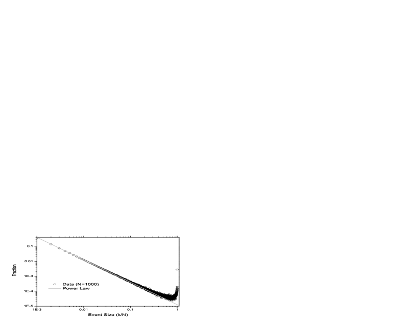
Figure 1: Distribution of event sizes for near mean field model simulation with $K_{R}=0$. Note the overabundance of large events.

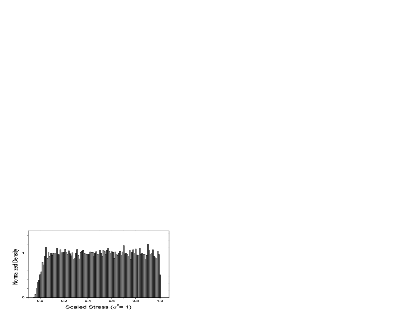
Figure 2: A histogram of stress values of sites in a typical near mean field simulation with uniform random residual stress between -0.05 and 0.05. The distribution has the statistical properties of a set of uniformly distributed random variables between 0.05 and 1.

If we assume the stress value of each site is independently sampled from such a uniform distribution, and order the results by increasing stress, we expect the stress gaps between nearest values to have an exponential distribution. Comparison of this theoretical distribution with an actual simulation (Fig. 3) show the assumption remarkably valid for large $N$. As long as there is a very small (Order $N^{-1}$) randomized residual stress, these stress statistics will be persistent in time and independent for each event. With no randomizing ingredient, limit cycles with time correlated distributions are possible.

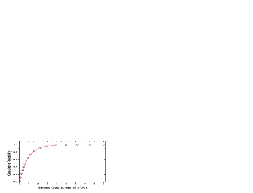
Figure 3: Comparison of simulated stress gap distribution with expectation from assuming independent uniformly distributed values. Plotted is the cumulative distribution of stress gaps (distance between nearest stress values) vs. cumulative exponential distribution.

Many ideas concerning the overabundance of large events in Fig. 2 have been put forward. This has often been considered an example of characteristic behavior, that is, repetition of an event whose size is determined by the local geometry. This can be considered a type of nucleation phenomena, a runaway Griffith rupture, where events larger than a critical size can not arrest.

This characteristic behavior is emphasized in dynamic weakening models Ben-Zion93 , where the increased propensity for a failed site to slip further (due to a weakened pinning force) is simulated by imposing a lower threshold stress $\sigma^{D}<\sigma^{F}$ for the duration of a single event. After a site fails it will receive stress transfer from subsequent failures, and thus may reach this lower threshold and fail again. Re-failing sites will contribute more to the external transfer and enhance the likelihood of continued rupture growth.

This form of weakening manifests itself after some failed sites have their stress brought back up to the dynamical threshold. This will only occur when the rupture reaches a certain size. After the onset of this dynamical weakening, the additional stress transfer typically results in a runaway event encompassing every block in the system. Thus, this form of weakening tends to produce characteristic events which always occur once the minimum rupture size is reached. To understand how the stress distribution and weakening rules determine the event size distribution and model behavior, we must examine the details of stress transfer between sites.

II.2 Stress Transfer

The above describes a series type dislocation where sites fail in sequence and the stress transfer occurs to other sites all at once. This makes it likely that any failing site (other than the single initiator) will have a stress slightly above the threshold, which subtly provides an order-of-failure dependence to the stress transfer. As a consequence, the exact stress transfer in simulation will depend on obscure factors like the order of iteration over sites. To eliminate this we must examine the stress transfer in more detail.

Suppose that in the course of an event there have been $k$ block failures. Let $\{k\}$ represent the set of indices of failed sites. Call $\kappa=k/N$ the fraction of failed sites. Then from (3) the change in stress for any stable site $i$ is

$$\Delta\sigma_{i\notin\{k\}} =\frac{1}{N}\sum_{j\in\{k\}}\Delta_{j}=\frac{\delta}{N}\sum_{j\in\{k\}}(\sigma_{j}^{f}-\sigma_{j}^{R})$$

$$=\delta\kappa\left(\left\langle\sigma^{f}\right\rangle_{k}-\left\langle\sigma^{R}\right\rangle_{k}\right)=\delta\kappa\left\langle-\Delta\sigma^{f}\right\rangle_{k}$$ (5)

where $\delta=(K_{R}+1-N^{-1})^{-1}$, and $\left\langle\cdot\right\rangle_{k}$ is an average applied over failed sites. We call this the external stress transfer to signify that it applies to sites that are not part of the rupture. The quantity $\sigma_{j}^{f}$ is the stress of site $j$ at failure, which may be greater than $\sigma^{F}$. Note that the slip displacement $\Delta_{j}$ is only dependent on the stress drop at failure because pinning occurs immediately, and subsequent stress changes will not cause this site to slip further. Since $\sigma^{f}$ is typically very near $\sigma^{F}$ and the $\sigma_{j}^{R}$ are identically distributed random variables, the term in parenthesis is on average independent of $k$. Thus the external transfer grows linearly with the fraction of failed sites.

To examine the effects of stress overshoot, suppose a site $j$ slips on the initial step. The external transfer is

$$\sigma_{i\neq j}=\sigma_{i}^{0}+\frac{\delta\left(\sigma_{j}^{0}-\sigma_{j}^{R}\right)}{N}$$ (6)

where for emphasis the superscript $0$ denotes the initial stress at a site before any failures have occurred. Of course, for the rupture initiator, $\sigma_{j}^{0}=\sigma^{f}=\sigma^{F}$. Now suppose this transfer causes sites $m$ and $n$ to fail. At this time $\sigma_{m,n}=\sigma_{m,n}^{0}+\delta\left(\sigma_{j}-\sigma_{j}^{R}\right)/N$, so after $m$ and $n$ fail the external transfer becomes

$$\sigma_{i\neq\{j,m,n\}}=\sigma_{i}^{0}+\frac{\delta\left(\sigma_{j}^{0}-\sigma_{j}^{R}\right)}{N}+\frac{\delta\left(\sigma_{m}^{0}-\sigma_{m}^{R}\right)}{N}+\frac{\delta\left(\sigma_{n}^{0}-\sigma_{n}^{R}\right)}{N}+\frac{2\delta^{2}\left(\sigma_{j}^{0}-\sigma_{j}^{R}\right)}{N^{2}}.$$ (7)

Note the factor of $2$ in the last term above comes from the fact that two sites ($m,n$) failed in the previous iteration. This simple stress transfer rule introduces dependence on which blocks fail during which iteration step. We would prefer the time evolution to be a transparent function of the initial stresses only. To satisfy this condition, we must make the stress transfer Abelian, that is, independent of the order of failure. This is similar in concept to the Abelian sand pile model Dhar90 ; Dhar99 . The key to making stress transfer Abelian is to use the additional degree of freedom offered with the inclusion of simulated weakening.

II.3 Forced Weakening

One way to visualize the effects of weakening is to examine the average stress of sites that have failed as a function of rupture size. After failure, a site has average stress $\left\langle\sigma^{R}\right\rangle$. Subsequent failures will transfer some stress to this now pinned site. Without weakening, the average stress of failed sites will grow with rupture size $\kappa$ as

$$\overline{\sigma_{int}}(\kappa)=\frac{\delta}{2}(\kappa-N^{-1})\left\langle\Delta\sigma\right\rangle_{k}.$$ (8)

With dynamic weakening, all failed sites with stress $\geq\sigma^{D}$ will fail again, putting a ceiling on the average internal stress, as illustrated in Fig. 4.

Figure 4: Schematic of average internal stress (average stress of sites that have failed) as a function of rupture size for several methods of simulated weakening.

We might imagine a different approach to weakening where failed sites shed a certain fraction of the stress they receive after failure by continuing to slide. This would not be convenient to simulate, but clearly possible. This would produce an average internal stress function the same as one for larger $K_{R}$, however now the stress difference is not dissipated, but transferred to external sites. The main point of this would be to generate a weakening effect present for all event sizes.  Implementing this ‘fractional weakening’ would involve re-computing the slip of all failed sites with each new failure. Instead, we might seek to formulate the model so the average internal stress function is given as a physical parameter and the requisite slips and stress transfer computed as a result. In essence, in place of deriving a weakening function from dynamical equations involving slip or velocity dependent friction, we can impose the effects of the weakening as they appear to stable sites. We call this approach forced weakening.

To arrive at a forced weakening formulation we first observe the change in stress of a site $j$ as it depends on $k$, the number of failed sites. Let $\Delta_{j}^{k}$ denote the slip displacement of site $j$ after $k$ failures. If it is nonzero it includes all block motion, including initial failure, additional failures from weakening, or continuous sliding. Consider the system of equations for the stress changes of the failed sites $j\in\{k\}$

$$\Delta\sigma_{j\in\{k\}}^{k} =\sigma_{j}^{k}-\sigma_{j}^{0}=-\delta\Delta_{j}^{k}+\frac{1}{N}\sum_{i\neq j\in\{k\}}\Delta_{i}^{k}$$

$$=-(K_{R}+1)\Delta_{j}^{k}+\frac{1}{N}\sum_{i\in\{k\}}\Delta_{i}^{k}$$ (9)

where $\sigma^{k}$ denotes the stress after $k$ failures (and $\sigma^{0}$ is the initial value). The last line demonstrates the simple linear form of the relationship between stress drops and slip displacements. This may be obtained via a matrix with diagonal elements $N^{-1}-(K_{R}+1)$ and off-diagonal elements $N^{-1}$. This matrix is easily inverted to obtain the slips $\Delta_{j}^{k}$ in terms of the current stress drops $\Delta\sigma_{j}^{k}$

$$\Delta_{j}^{k} =\frac{-(K_{R}+1-k/N)\Delta\sigma_{j}^{k}-N^{-1}\sum_{i\in\{k\}}\Delta\sigma_{i}^{k}}{(K_{R}+1)\left(K_{R}+1-k/N\right)}$$

$$=\frac{-\Delta\sigma_{j}^{k}}{K_{R}+1}-\frac{(k/N)\ \left\langle\Delta\sigma^{k}\right\rangle_{k}}{(K_{R}+1)\left(K_{R}+1-k/N\right)}$$ (10)

This expression provides the slips that are necessary to generate a set of stress drops.

The slips are directly related to the external transfer, as in (5). Summing over them yields a new expression for the external transfer in terms of the stress drops.

$$\Delta\sigma_{i\notin\{k\}} =\frac{1}{N}\sum_{j\in\{k\}}\Delta_{j}=\frac{k}{N}\left\langle-\Delta\sigma^{k}\right\rangle_{k}$$

$$\times\left[\frac{1}{K_{R}+1}+\frac{k/N}{(K_{R}+1)(K_{R}+1-k/N)}\right]$$

$$\Delta\sigma_{i\notin\{k\}} =\frac{\kappa}{(K_{R}+1-\kappa)}\left\langle-\Delta\sigma^{k}\right\rangle_{k}$$ (11)

This is identical to (5) when $k=1$. However, the new effective transfer coefficient $\delta(\kappa)=(K_{R}+1-\kappa)^{-1}$ grows with the rupture size. Making up for this is the fact that the stress drops are no longer computed only at failure, but account for stress changes occurring as the rupture progresses. As failed sites pin and acquire additional stress transfer, the average change in stress will decrease. Observe that to calculate the external transfer, we need not specify individual stress drops or slips, but require only the average dynamic stress drop of all failed sites. This evolving average stress drop is defined as

$$\left\langle-\Delta\sigma^{k}\right\rangle_{\kappa} =\frac{1}{k}\sum_{j\in\{k\}}(\sigma_{j}^{0}-\sigma_{j}^{k})$$

$$=\left\langle\sigma^{0}\right\rangle_{\kappa}-\overline{\sigma_{int}}(\kappa)$$ (12)

where we have defined the average internal stress (AIS) function $\overline{\sigma_{int}}(\kappa)=\left\langle\sigma^{k}\right\rangle_{k}$, which characterizes the frictional weakening. The stress transfer now depends only on the average initial stress of failed sites (which decreases with rupture size) and the AIS function. Both may be defined in terms of rupture size independent of a particular update algorithm. Using this formulation, avalanches are Abelian.

In numerical simulation, we must eventually assign an actual slip and/or residual stress to each failed site. Care must be taken to make results agree with the analogous forward simulation. For example, given a linear AIS function $f(\kappa)=\alpha\kappa+\beta$, we could assign the $k^{th}$ failed site a random residual stress (with mean $\beta$) plus $2\alpha(k-1)/N$. When using AIS functions with no forward equivalent, the method of assigning final stresses must be stated explicitly.

The forced weakening method has two main advantages. Practically, it allows the simulation of models with arbitrary weakening characteristics, most of which would not be obtainable with modified CA rules. Formally, the model is Abelian, so that the event size is a unique function of the initial stress configuration. Using this fact we can seek an expression which will determine the event size given adequate information of the initial stresses.

III Model Analysis

With an Abelian stress transfer, the final event size depends only on the initial stress distribution. We could therefore compute the final event size if we concretely characterize the stress distribution. For model solutions we find it convenient to mostly work with the stress deficits defined as

$$\Sigma_{i}(t)=\sigma^{F}-\sigma_{i}(t)$$ (13)

representing the distance a site $i$ is from failure. A rupture originates at sites where $\Sigma=0$ and advances through sites with progressively larger values of $\Sigma$. Consider the cumulative distribution $P_{\Sigma}(\chi)$ defined as the fraction of sites with stress deficit $\Sigma\leq\sigma^{F}\chi$ (scaled so $\chi$ varies from zero to one). Typically, one would choose the microscopic length $a$ such that $K_{C}a=\sigma^{F}$ so that $\sigma^{F}=1$. For a specific stress configuration $P_{\Sigma}(\chi)$ will be a piece-wise continuous function with $N$ steps.

III.1 Solution for Rupture Size

To express the stress transfer as function of rupture size, the discrete initial stresses $\sigma_{j}$ must be expressed in terms of the stress distribution. Beginning with the forced weakening form of the external transfer $\tau(\kappa)$,

$$\tau(\kappa)=\frac{\kappa}{K_{R}+1-\kappa}\left\langle-\Delta\sigma^{k}\right\rangle_{\kappa}.$$ (14)

where $\left\langle-\Delta\sigma^{k}\right\rangle_{\kappa}=k^{-1}\sum_{j\in\{k\}}(\sigma_{j}^{0}-\sigma_{j}^{k})$, we notice that the $k^{th}$ site to fail in the rupture has a stress deficit of $P_{\Sigma}^{-1}(\frac{k-1}{N})$. The factor $k-1$ reflects the fact that the first site to fail has a stress deficit of zero, so $P_{\Sigma}(0)=N^{-1}$, and $P_{\Sigma}^{-1}(\eta<N^{-1})$ is undefined. This relationship is illustrated graphically in Fig. 5. Using this fact we may write the average stress drop in (14) as

$$-\left\langle\Delta\sigma^{k}\right\rangle_{k} =\frac{1}{k}\sum_{j\in\{k\}}(\sigma_{j}^{0}-\sigma_{j}^{k})=\sigma^{F}-\frac{1}{k}\sum_{j\in\{k\}}\left(\sigma^{F}-\sigma_{j}^{0}+\sigma_{j}^{k}\right)$$

$$=\sigma^{F}-\frac{1}{\kappa}\sum_{j\in\{k\}}\frac{1}{N}\left(\Sigma_{j}^{i}+\sigma_{j}^{k}\right)$$

$$=\sigma^{F}-\frac{\sigma^{F}}{\kappa}\int_{\varepsilon}^{\kappa}P_{\Sigma}^{-1}(\eta-\varepsilon)d\eta-\overline{\sigma_{int}}(\kappa)$$ (15)

where we have identified the average internal stress function $\left\langle\sigma^{k}\right\rangle_{k}=\overline{\sigma_{int}}(\kappa)$ and introduced the notation $\varepsilon=N^{-1}$. Note that we took no limit in writing the integral, but recognized the equivalent of the sum and an integral over a step function.

Using this form of the average stress drop we may write the external transfer in terms of the stress distribution as

$$\tau(\kappa)=\frac{1}{K_{R}+1-\kappa}\left[\kappa\sigma^{F}-\kappa\overline{\sigma_{int}}(\kappa)-\sigma^{F}\int_{\varepsilon}^{\kappa}P_{\Sigma}^{-1}(\eta-\varepsilon)d\eta\right].$$ (16)

Using (16) and the statistical properties of $P_{\Sigma}^{-1}(\eta)$, we should be able to calculate the size of the next event. At any point during a sequence of failures, a rupture will arrest if every (initial) stress deficit in the unfailed region is greater than the current external transfer. Referring to Figure 5, we see that the stress deficit of the next site to fail is $P_{\Sigma}^{-1}(\kappa)$. Using this we define a stress excess $v$ which will provide a criteria for the progress of an event in terms of the stress distribution:

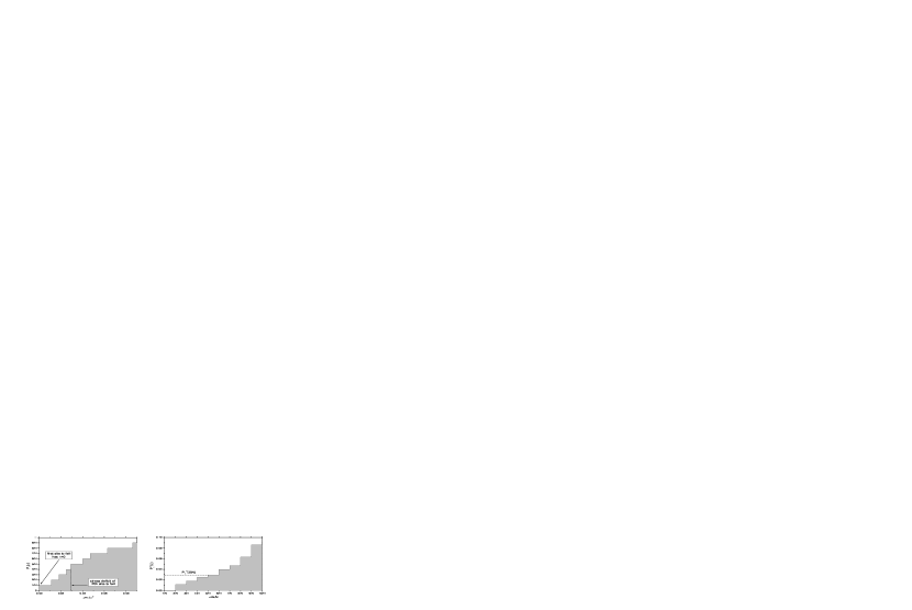
Figure 5: Relationship between inverse cumulative stress deficit function $P_{\Sigma}$ and event size $\kappa=k/N$. A rupture must initiate at a site where $\Sigma=0$, so the stress deficit of the $k^{th}$ site to fail is given by $P_{\Sigma}(\kappa-N^{-1})$.

$$v(\kappa)=\tau(\kappa)-\sigma^{F}P_{\Sigma}^{-1}(\kappa).$$ (17)

When $v$ is positive, a rupture will continue to grow, arresting only if/when $v(\kappa)=0$. Assuming a rupture has initiated, setting the stress excess to zero yields an integral equation for the final rupture size $\kappa$:

$$\frac{1}{K_{R}+1-\kappa}\left[\kappa\sigma^{F}-\kappa\overline{\sigma_{int}}(\kappa)-\sigma^{F}\int_{\varepsilon}^{\kappa}P_{\Sigma}^{-1}(\eta-\varepsilon)d\eta\right]-\sigma^{F}P_{\Sigma}^{-1}(\kappa)=0$$ (18)

To solve this equation it would be convenient to consider $\kappa$ a truly continuous variable. The stress distribution could vary continuously if we let $N\rightarrow\infty$, or by averaging the stress deficits over a short time interval. The latter works if we imagine the system driving and stress transfers to be continuous, so all intermediate values of stress are passed through during updates. This form of temporal course-graining has been central to previous analysis of slider-block models Klein99 .

III.2 Example Solutions

It is instructive to examine the stress excess function and the event size solutions when we can perform the integral over the step function analytically; that is, when the steps are of equal size. In this case the stress deficit values are $\Sigma_{1}=0,$ $\Sigma_{2}=1/N$, $\Sigma_{3}=2/N$, etc. This will also represent the case where $N\rightarrow\infty$, and the empirical distribution of values is identical to the probability distribution of a single variable, and the integrals are taken over a continuous variable. However, we will not take this limit so factors of $\varepsilon=N^{-1}$ are apparent. In this discrete formulation, the integrals become reducible sums.

As we observed, in a system exhibiting power law behavior, the stresses are distributed as if they were selected from a uniform distribution. Fore simplicity, we can ignore the small variation from the uniform distribution due to random residual stresses, since this anomaly will only be encountered for ruptures nearly the size of the system. Thus we take $p_{\Sigma}(\chi)=1$, $P_{\Sigma}(\chi)=\kappa$, and $P_{\Sigma}^{-1}(\kappa)=\chi$.

III.2.1 Perfect Weakening

We will first examine the rather artificial scenario of perfect weakening, where no additional stress beyond the residual noise may be supported by failed sites. This is achieved by imposing a constant average internal stress $\overline{\sigma_{int}}(\kappa)=0.$

The physical interpretation of this perfect weakening scenario is much like a democratic fiber bundle model Anderson97 . Imagine a cable composed of several parallel axial fibers under tension, with a gradually increasing load. In this model the individual fibers have some randomly distributed strength at which they will break. When a fiber breaks, the load it was bearing is distributed equally among all the remaining fibers.

In the context of a slider block model, failed blocks do not re-pin during a rupture, and continue to slide with stress changes from additional failures. The distribution of fiber strengths corresponds to the distribution of stress deficits in our system. The factor of $1-\kappa$ in the denominator of the stress transfer is equivalent to the rule of sharing the load only among unbroken fibers. This earthquake model adds the possibility of stress dissipation through the $K_{R}$ parameter. When $K_{R}=0$ the models are equivalent.

The stress excess function for perfect weakening is shown in Fig. 6. Determining the rupture size from (18) yields the equation

$$\kappa^{2}=(2K_{R}-\varepsilon)\kappa$$ (19)

which has solutions for $\kappa=0$ or $\kappa=2K_{R}-\varepsilon$. For $K_{R}<\varepsilon$ the stress excess is always positive and the rupture will run away. For slightly larger values of $K_{R}$ the stress excess function starts negative and crosses the axis a short distance from zero, as stress dissipation kills the rupture within the first few failures. After crossing zero the function again increases without limit. Larger values of $K_{R}$ do not produce critical event size distributions so aren’t of interest. With perfect weakening, ruptures of significant size will never arrest.

III.2.2 No Weakening

Now consider a model with a linear AIS function, equivalent to typical slider-block models with no weakening:

$$\overline{\sigma_{int}}(\kappa>0)=\delta\frac{(\kappa-\varepsilon)}{2}.$$

The solution to the rupture size equation is now

$$\kappa^{2}=\kappa(2+2K_{R}-\varepsilon)$$ (20)

which has solutions at $\kappa=0$ and near $\kappa=2$ for small $K_{R}$. More important, however, is the behavior of the stress excess function below $\kappa=1$. Again the critical value of $K_{R}$ is $\varepsilon$: for $K_{R}<\varepsilon$, the initial stress excess is positive and remains so up to $\kappa=1$, so again any rupture that initiates will run away (the model is super-critical). For $K_{R}>\varepsilon$, the stress excess is always negative, and no rupture will form (Fig. 6).

However, when $K_{R}\rightarrow\varepsilon$ the stress excess function vanishes for all $\kappa$. In this case, we have a critically propagating rupture, with the exact stress necessary to tumble each site in succession. Also, notice in Fig. 6 how closely the stress excess remains to zero when $K_{R}$ is of order $\varepsilon$. In this case small fluctuations in the stress distribution could generate a transient positive stress excess, resulting in a finite rupture size.

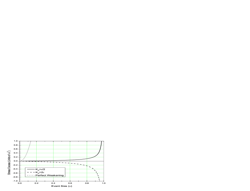
Figure 6: Ideal stress excess functions for models with perfect weakening and no weakening.

III.2.3 Dynamic Weakening

Dynamic weakening can be treated with a combination of the above two cases: as long as the external transfer is below the dynamic stress threshold, there is no weakening. Once external transfer crosses the dynamic threshold, the average internal stress function becomes a constant, resulting in runaway stress excess as in the perfect weakening scenario. The point at which this crossover happens is easy to calculate by setting $\tau(\kappa)=\sigma^{D}/\sigma^{F}$. For $W=0$ and $K_{R}=0$, this yields a crossover point at $\kappa=\sigma^{D}/\sigma^{F}$, which is no surprise. Nonzero values of $W$ or $K_{R}$ result in slightly larger values of the crossover point.

III.2.4 Fractional Weakening

The fractional weakening AIS function is identical to that of no weakening with a modified slope. With no weakening the slope is $\delta/2$, which depends on $K_{R}$.  Fractional weakening can effectively balance the effect of dissipation, moving the critical value of $K_{R}$ up. Other conclusions of the case with no weakening remain the same.

Using these ideal solutions we can easily understand the role of the control parameters and weakening function in terms of how a single event propagates. Clearly, without fluctuations in the stress distribution, the model behavior is trivial. Now we will examine solutions for finite models where the time-averaged stress distribution is a stochastic process.

IV Fluctuations and Stochastic Rupture Propagation

When using a smooth stress distribution the solutions for the rupture size are trivial, producing no complexity. Passing to the thermodynamic limit yields a model with no fluctuations in the stress distribution, a true mean field model. This is not what we observe in simulation, as actual stress distributions are finite realizations. A model with a finite number of elements, no matter how large, is inherently different from an infinite model. The finite $N$ and consequent course grained empirical distribution provides the inherent discreteness necessary to produce complex behavior, a near mean field model.

In a short time interval $\Delta t$ where no failures occur, the stress at each site changes an amount $\Delta\sigma=(K_{R}+1)V\Delta t$ where $V$ is a velocity measured in units of the microscopic length $a$ per unit time. A time average is equivalent to specifying $P_{\Sigma}(\chi)$ as the integral of a density function $p_{\Sigma}(\chi)$, which is the average number of sites with stress deficit $\Sigma$ between $\sigma^{F}\chi$ and $\sigma^{F}(\chi+\Delta\chi)$, where $\Delta\chi$ is the change in scaled stress $(\Delta\sigma/\sigma^{F})$ over the time interval. For a stress distribution of normalized width $I$ $(0<I\leq 1)$, the expected time to the next event is defined by $\Delta\chi=I/N$, or $\Delta t=I/[NV(K_{R}+1)]$.

Based on the mean field distribution of event sizes the expected event size at any time is $k=\sqrt{N}$. Thus, during the average time interval between events, we expect the distribution function to average over $\sqrt{N}$ different stress values. For large $N$, this should be adequate to define a stress distribution function as a stochastic process with well defined mean and variance at each point. If we use this statistical description of the stress distribution, we will obtain a statistical answer for the event size.

The near mean field model preserves the essential fluctuations characteristic of discrete models, while also proving analytically tractable. The stress distribution averaged over the inter-event time is a stochastic process, and computing the event size from this will yield a probability distribution. Since we observe the stress distribution is statistically stationary, the distribution of event sizes for any time step is also the time-average distribution.

Again consider the case where the stresses (or stress deficits) appear to have been chosen from a uniform distribution. Consider an ordering of stress deficits $\Sigma_{1}<\Sigma_{i}<\ldots<\Sigma_{N}$ and define $\Sigma_{1}=0$ and $\Sigma_{N+1}=1$. Let $Y_{i}=\Sigma_{i+1}-\Sigma_{i}$ for $i=1\ldots N$. Then we would expect the gaps $Y_{i}$ to be independent identically distributed (i.i.d.) random variables with an exponential distribution of mean $\mu_{Y}=N^{-1}$ and variance $\operatorname{Var}Y=N^{-2}$ (taking $W=0$ for simplicity). Derivations of the event size distribution from these statistics have been considered before Dahmen98 ; Ding93 , but the forced weakening formulation provides new rigor and generality in the results. We will also derive the finite-size correction to the mean field power law behavior for the first time.

Notice that the partial sum over intervals is nothing but the inverse cumulative distribution,

$$\sum_{i=1}^{k}Y_{i} =\Sigma_{k+1}-\Sigma_{1}$$

$$=P_{\Sigma}^{-1}(\frac{k}{N})$$ (21)

yielding the stress deficit of the $k^{th}$ site to fail.

Next define the zero mean random variables

$$X_{k/N} =\frac{\sum_{i=1}^{k}(Y_{i}-\mu)}{\sigma\sqrt{N}}$$

$$=\sqrt{N}\sum_{i=1}^{k}Y_{i}-\frac{k}{\sqrt{N}}$$ (22)

that are partial sums of the gaps up to the $k^{th}$ site. As $N\rightarrow\infty$ the intervals $X_{t^{\prime}}-X_{t}$ are Gaussian random variables with mean zero and variance $t^{\prime}-t$. This is a standard method of constructing a Wiener process from any underlying i.i.d. sequence of random variables. Since we aren’t actually taking the infinite $N$ limit, we should consider this process equivalent to a Wiener process at scales much greater than $N^{-1}$.

Knowing that the $X_{t}$ represents a Brownian motion in the continuum limit we may express the inverse cumulative distribution as

$$P_{\Sigma}^{-1}(\kappa) =\sum_{i=1}^{k}Y_{i}=\left(\frac{X_{k/N}}{\sqrt{N}}+\frac{k}{N}\right)$$

$$=\frac{X_{\kappa}}{\sqrt{N}}+\kappa$$ (23)

Thus the inverse cumulative distribution may be presented as a sum of the ideal linear term (drift) and a Wiener process with variance $N^{-1}$. Note that the fluctuations scale with the system size as expected.

The stress excess function also depends on the integral of the inverse cumulative distribution, representing the average stress deficit of failed sites

$$\kappa\left\langle\Sigma\right\rangle_{\kappa} =\int_{0}^{\kappa}P_{\Sigma}^{-1}(\chi)d\chi=\frac{\kappa^{2}}{2}+\frac{1}{\sqrt{N}}\int_{0}^{\kappa}X_{\chi}d\chi$$ (24)

$$=\frac{\kappa^{2}}{2}+S_{\kappa}$$ (25)

This integral introduces a new process $S_{\kappa}$. This is a sum of independent Gaussian random variables with zero mean. The result is a random variable with zero mean and a variance $\kappa^{3}/3N+\mathcal{O}(1/N^{2})$ Preston01 . This term does not bias the stochastic component, and for large $N$ it’s contribution will be negligible next to $X_{k}/\sqrt{N}$.

The stress excess function now becomes

$$\frac{v(\kappa)}{\sigma^{F}}=\frac{1}{K_{R}+1-\kappa}\left[\kappa-\kappa\frac{\overline{\sigma_{int}}(\kappa)}{\sigma^{F}}-\frac{\kappa^{2}}{2}-S_{\kappa}\right]-\kappa-\frac{X_{k}}{\sqrt{N}}.$$ (26)

First examine the behavior of this stochastic function near $\kappa=0$. Consider the critical model ($K_{R}=N^{-1}$) with no weakening. In studying (20) we saw this function vanishes for all values of $\kappa$. Only the noise terms, dominated by $X_{\kappa}/\sqrt{N}$, are present. Thus, the distribution of event sizes is the distribution of zero-crossings of a standard random walk.

IV.1 Event Size Distributions

The zero-crossing distribution is easily derived using the fact that any i.i.d. distribution can be used to construct the Wiener process with identical results. It’s convenient to build the walk from a discrete random variable taking values of $\pm 1$ with equal probability. Let $P_{d}(k)$ denote the probability that the walk is $d$ steps from the origin after $k$ steps are taken. Taking the (horizontal) step size of the walk to be $1/2N$, returns to zero are possible at steps $k/N$ with probability

$$P_{0}(k)=\frac{1}{2^{2k}}\frac{(2N-2)!}{(N-1)!^{2}}$$ (27)

The probability of $k$ being the first crossing of zero is $P_{0}(k)/k$. These probabilities have a power law distribution as seen by taking the log and applying Stirling’s approximation:

$$\frac{P_{0}^{k}}{k}\simeq\frac{k^{-3/2}}{N^{3/2}\sqrt{2\pi}}$$ (28)

The result is a power law with an exponent of $-3/2$ as observed in Fig. 1. This distribution matches the power law behavior observed in simulation, except at the largest values.

The expected distance $d$ from the origin for an unbiased random walk in terms of the number of steps $k$ is given by $\left\langle d_{k}\right\rangle\simeq\sqrt{k\pi/2}$ for large $k$. With our distance per step of $1/\sqrt{N}$, the expected magnitude of the walk grows as $\sqrt{\pi\kappa/2}$. However, all the stress gaps must add to one (minus the $\mathcal{O}(1/N)$ distance $\sigma^{F}-\Sigma_{N}$), so the walk must be constrained to return to zero at $\kappa=1$. If the stress values are considered a Poisson point process, this is equivalent to requiring there to be exactly $N$ values between $0$ and $\sigma^{F}$. For $N\gg 1$, this constraint is unnoticeable in the statistics of individual stress gaps, but manifests itself when all the gaps are summed.

To correct this we weight each probability $P_{0}(k)$ by the probability that a walk starting at that point will return to zero at $k=N.$ This latter quantity is $P_{0}(N-k)$. Dividing the product of these terms by $P_{0}(N)$ provides the proper normalization. The resulting constrained distribution $P_{0}^{\prime}(k)$ is given by

$$P_{0}^{\prime}(k)=\frac{(2k)!(2N-2k)!N!^{2}}{(2N)!(N-k)!^{2}k!^{2}}.$$ (29)

The approximated first passage distribution $P_{0}^{\prime}(k)$ is shown in Fig. 7. This is well approximated by a corrected power law

$$P_{0}^{\prime}(\kappa)=\frac{\kappa^{-3/2}}{\sqrt{2\pi}\sqrt{1-\kappa}}.$$ (30)

Note this has a minimum at exactly $\kappa=3/4$. We conclude that this feature, which resembles a nucleation phenomenon, stems from the basic statistics of the stress distribution. For models with a large number of sites, the low number of large events often makes it difficult to compare the data to an exact power law. However, we can also compare the cumulative stress distribution the the integral of (30). This is shown in Fig. 8. However, a discrepancy at small event sizes, due to error in Stirling’s approximation is evident in this graph. Using the exact combinatorial expression (29) instead yields a perfect fit to the simulation data.

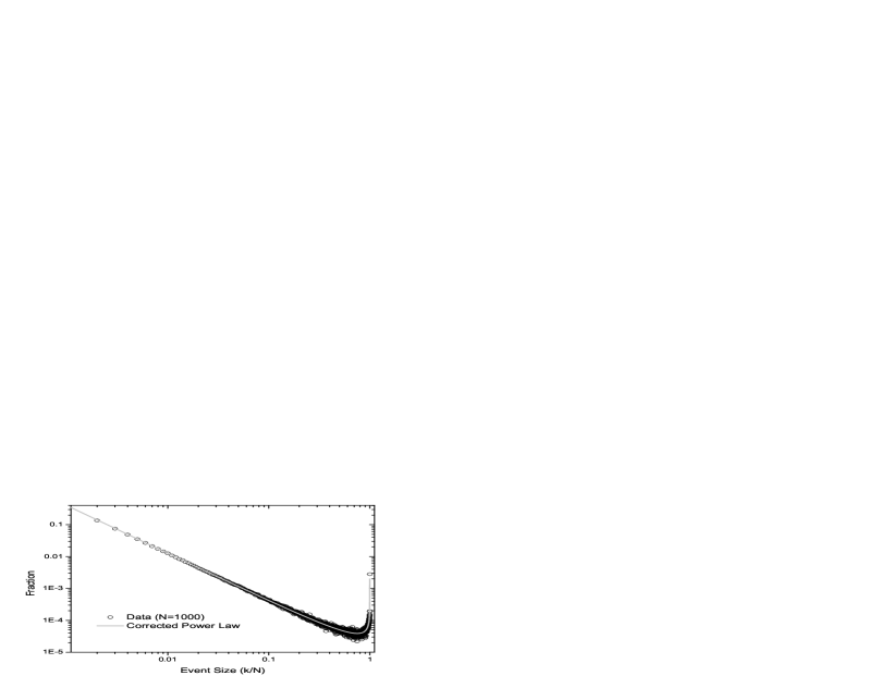
Figure 7: Theoretical event size distribution for a no-weakening critical model with the additional constraint on the stochastic component of the stress distribution. This results in an exact fit to the simulation data.

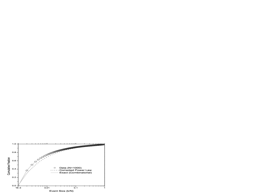
Figure 8: The Cumulative distribution of events compared to the theoretical power law. Discrepancies for small events show the limits of Stirling’s approximation. Using the combinatorial expression yields an exact fit to simulation data.

Note in this particular case we can also derive the distribution from first principles, since each site contributes exactly $1/N$ to the stress transfer, when the rupture arrests there must be exactly $k$ sites in an interval $k/N$, which for $N$ uniformly distributed variables can be written

$$P^{\prime}(k)=\frac{1}{k}\left(\begin{array}[c]{c}N\\ k\end{array}\right)\left(\frac{k}{N}\right)^{k}\left(1-\frac{k}{N}\right)^{N-k}.$$ (31)

However, the above treatment is more general, and may be used to consider the distribution of event sizes for non-critical models.

When $K_{R}>\varepsilon$, The idealized stress excess is negative (and diverges at $\kappa=K_{R}+1$). The magnitude of the stochastic term must overcome this deficit for a rupture to propagate. A previous approach Dahmen98 is to linearize the stress excess about $\kappa=0$ (not including terms of $\mathcal{O}(\varepsilon)$)

$$v(\kappa)\simeq-\frac{K_{R}}{1+K_{R}}\kappa-\frac{X_{\kappa}}{\sqrt{N}}$$ (32)

and compute the first crossings of the random walk with the line. The exact result is given by the Bachelier-Levy formula Lerche86 . We can derive the result by defining a biased walk where an step up has probability $p=\frac{1}{2}-\frac{c}{\sqrt{N}}$ and a step down $q=\frac{1}{2}+\frac{c}{\sqrt{N}}$, where $c=\frac{K_{R}}{2(K_{R}+1)}$. The first crossing probabilities for $k=1,2,\ldots$ are

$$\frac{P_{0}(k)}{k}=\frac{1}{k}\frac{(2k)!}{k!^{2}}\left(\frac{1}{4}-\frac{c^{2}}{N}\right)^{k}\thicksim k^{-3/2}e^{-4c^{2}\kappa},\;N>>1.$$ (33)

For the limiting value of $c=1/2$ ($K_{R}\rightarrow\infty$), the power law is dominated by an exponential decay $e^{-\kappa}$.

However, the linearized stress excess does not provide a valid approximate solution. The actual distribution will be truncated much more quickly. Ignoring terms of $\mathcal{O}(\varepsilon)$ we can write the entire expression for the stress excess

$$\nu(\kappa) \simeq-\frac{K_{R}}{K_{R}+1}\kappa-\frac{K_{R}}{2(K_{R}+1)(K_{R}+1-\kappa)}\kappa^{2}$$

$$=-\frac{K_{R}}{2}\left[\frac{\kappa}{K_{R}+1}+\frac{\kappa}{K_{R}+1-\kappa}\right]$$ (34)

Note that the magnitude of the nonlinear term overtakes the first when $\kappa>(K_{R}+1)/2$. The second line gives the stress excess function in its most compact form.

If we label the non-stochastic part of the stress excess $\nu(\kappa)=\nu^{\prime}(\kappa)+X_{\kappa}/\sqrt{N}$, the event size distribution can be formulated as the distribution of first intersection (Fig. 9).

Figure 9: Event size distributions for simulations with $K_{R}>\varepsilon$. Also shown is the theoretical distribution based on the linearized stress excess for $K_{R}=1$. The data falls off much more rapidly due to the nonlinear term.

$$X_{\kappa}=\sqrt{N}\,\left|\nu^{\prime}(\kappa)\right|$$ (35)

where we recognize the sign of the walk term is irrelevant. There is an extensive literature regarding the intersection of a random walk with a curvilinear boundary Lerche86 ; Durbin85 . Several formal solutions are available, but analytic forms exist only for special cases. Numeric computation based on the formal solution is still useful because it eliminates sampling errors for low probability events.

V Conclusions

The forced weakening method introduces a means of modeling dynamical behavior leading to an instability in an efficient discrete time simulation. This is done by using an arbitrary weakening function to compute stress transfers during simulation, then assigning random residual stresses consistent with the weakening function at the completion of rupture. This technique results in Abelian avalanches allowing a rigorous and implementation-independent analysis. Event distributions derived from this analysis yield excellent agreement between theory and simulation, including a novel explanation for the overabundance of large events. If one used a small-scale dynamical model to characterize the average internal stress of a rupture as it depends on the physical parameters of a rate and state dependent frictional law, we could understand features of the resulting event size distribution.

This approach should be equally applicable to related discrete threshold models. While the resulting formalism is dependent on the mean-field character of the model, the numerical techniques may find wider use whenever an inversion like (10) is available. Use of a stress excess function to understand the event size distribution may be extendible to non mean field models with a finite interaction range. Local correlations might result in the stochastic component resembling a fractional Brownian motion, predictably altering the crossing distribution.

E.F.P. and J.B.R. acknowledge support by DOE grant DE-FG03-95ER14499; J.S.S.M. was supported as a Visiting Fellow by CIRES, University of Colorado at Boulder.

References

- (1) R. Burridge and L. Knopoff, Bull. Seismol. Soc. Am. 57, 341 (1967)
- (2) J. B. Rundle and D. D. Jackson, Bull. Seismol. Soc. Am. 67, 1363 (1977)
- (3) H. Nakanishi, Phys. Rev. A 43, 6613 (1990)
- (4) C. D. Ferguson, Ph.D. Dissertation, Boston University 1997
- (5) D. S. Fisher, Phys. Rev. B 31, 1396 (1985)
- (6) T. Giamarchi and P. LeDoussal, Phys. Rev. B 52, 1242 (1995)
- (7) D. Ertas and M. Kardar, Phys. Rev. E 49, R2532 (1994)
- (8) K. Dahmen, D. Ertas, and Y. Ben-Zion, Phys. Rev. E 58, 1494 (1998)
- (9) C. D. Ferguson, W. Klein, and J.B. Rundle, Phys. Rev. E 60, 1359 (1999)
- (10) E. F. Preston et. al., Computing in Science and Engineering 2(3), 34, (2000)
- (11) E. J. Ding and Y. N. Lu, Phys. Rev. Let. 70, 3627 (1993)
- (12) D. Dhar, Phys. Rev. Let. 64, 1613 (1990)
- (13) D. Dhar, Physica A 263, 4 (1999)
- (14) J. V. Andersen, D. Sornette, and K.T. Leung, Phys. Rev. Let. 78, 2140 (1997)
- (15) Y. Ben-Zion and J. R. Rice, J. Geophys. Res. 98, 14,109 (1993)
- (16) E. F. Preston, Ph.D. Dissertation, University of Colorado, 2001
- (17) H. R. Lerche, Boundary Crossing of Brownian Motion, Springer-Verlag, New York, 1986
- (18) J. Durbin, J. Appl. Prob. 22, 99-122 (1985)