The Fermi-Ulam Accelerator Model Under Scaling Analysis

Abstract

The chaotic low energy region of the Fermi-Ulam simplified accelerator model is characterised by use of scaling analysis. It is shown that the average velocity and the roughness (variance of the average velocity) obey scaling functions with the same characteristic exponents. The formalism is widely applicable, including to billiards and to other chaotic systems.

Enrico Fermi ref1 attempted to describe cosmic ray acceleration through a mechanism in which a charged particle can be accelerated by collision with a time dependent magnetic field. His original model was later modified and studied in different versions, based on different approaches, one of which is the well-known problem of a bouncing ball or Fermi-Ulam model (FUM) ref3 ; ref4 . The main results for this version of the problem, considering periodic oscillation, can be summarised as: (i) it is described via the formalism of an area-preserving map; (ii) it presents a set of invariant spanning curves in the phase space for high energy; (iii) a set of KAM islands surrounded by a chaotic sea can be observed in the low energy regime; and (iv) small chaotic regions limited by two different invariant spanning curves can be observed at intermediate energies. A related version of this problem in a gravitational field, sometimes referred to as a bouncer ref8 , presents a property, in contradistinction to the bouncing ball problem, that depending on both initial conditions and control parameters, the particle has unlimited energy gain i.e. the basic condition needed for Fermi acceleration. The difference between these apparently very similar models was latter clarified by Lichtenberg et al ref9 . The quantum problems corresponding to both the FUM and bouncer models have also been investigated ref10 ; ref11 ; Referee . The special interest in studying these one-dimensional classical systems arises because they allow direct comparison of theoretical predictions with experimental results ref11a ; ref11b . Even more, the formalism used in the characterisation of such models can immediately be extended to the so-called billiards class of problems ref17 ; ref18 ; ref19 .

In this Letter, we characterise the average velocity, and its variance which we will refer to as roughness, within the chaotic sea of the phase space using scaling functions. One of our tools, the roughness, is an extension of the formalism used to characterise rough surfaces barabasi which, as we will show, is immediately applicable to chaotic orbits in the problem of time dependent potential wells ref12 ; ref13 ; ref14 ; ref15 as well as to billiards problems ref16 ; ref16a . This scaling scenario represents the first characterisation of the integrability-chaos transition in this problem and should be applicable to several billiard problems. The formalism may therefore prove useful in characterising classes of universality.

Let us describe the system and how to characterise its dynamical evolution. It consists of a classical particle bouncing between two rigid walls, one of which is fixed; the other moves periodically in time with a normalised amplitude $\epsilon$. We will describe the system using a map $T(V_{n},\phi_{n})=(V_{n+1},\phi_{n+1})$ which gives the new velocity of the particle and the corresponding phase of the moving wall immediately after the particle suffers a collision with it. We will use a simplification ref20 in our description of this problem: we will suppose that both walls are fixed but that, when the particle suffers a collision with one of the walls, it exchanges momentum as if the wall were moving. This simplification carries the huge advantage of allowing us substantially to speed up our numerical simulations compared with the full model. It is usefully applicable because the main dynamical properties of the system are preserved under such conditions. Incorporating this simplification in the model and using dimensionless variables, the map is written as ref3

$$T:\left\{\begin{array}[]{ll}V_{n+1}=|V_{n}-2\epsilon\sin(\phi_{n+1})|{}{}\\ \phi_{n+1}=\phi_{n}+{2\over{V_{n}}}~{}~{}~{}{\rm mod}2\pi\\ \end{array}\right..$$ (1)

The term $2/V_{n}$ specifies the length of time during which the particle travels between collisions, while $-2\epsilon\sin(\phi_{n+1})$ gives the corresponding fraction of velocity gained or lost in the collision. The modulus function is introduced to avoid the particle leaving the region between the walls. We stress that the approximation of using the simplified FUM is valid in the limit of small $\epsilon$. So, the transition from integrability ($\epsilon=0$) to chaos ($\epsilon\neq 0$), characterising the birth of the chaotic sea, can be well described.

We will concentrate on the scaling behaviour present in the chaotic sea. We investigate the evolution of the velocity averaged in $M$ initial phases, namely

$$V(n,\epsilon,V_{0})={1\over M}\sum_{j=1}^{M}V_{n,j}~{}~{},$$ (2)

where $V_{0}$ is the initial velocity and $j$ refers to a sample of the ensemble. In order to define the roughness barabasi , we first consider the average of velocity over the orbit generated from one initial phase

$$\overline{V}(n,\epsilon,V_{0})={1\over{n}}\sum_{i=0}^{n}V_{i}~{}.$$ (3)

We then evaluate the interface width around this averaged velocity. Finally, the roughness is defined by considering an ensemble of $M$ different initial phases:

$$\omega(n,\epsilon,V_{0})\equiv{1\over{M}}\sum_{j=1}^{M}\left[\sqrt{\overline{V^{2}}_{j}(n,\epsilon,V_{0})-\overline{V}_{j}^{2}(n,\epsilon,V_{0})}~{}\right].$$

Fig. 1 shows the behaviour of the roughness for two different control parameters.

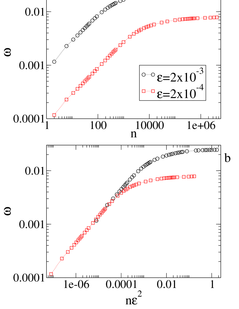
Figure 1: (a) Behaviour of the roughness $\omega$ as a function of the iteration number $n$. (b) Behaviour of $\omega$ as a function of $n\epsilon^{2}$. Both curves were derived from an ensemble average of $50,000$ different initial conditions starting with $V_{0}\approx 0$.

We can see in Fig. 1(a) that the roughness grows for small iteration number $n$ and then saturates at large $n$. The change from growth to saturation is characterised by a crossover iteration number $n_{x}$.

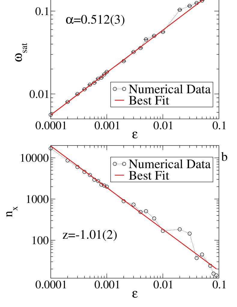
Figure 2: (a) Plot of $\omega_{\rm sat}$ against the control parameter $\epsilon$. (b) The crossover iteration number $n_{x}$ as a function of $\epsilon$.

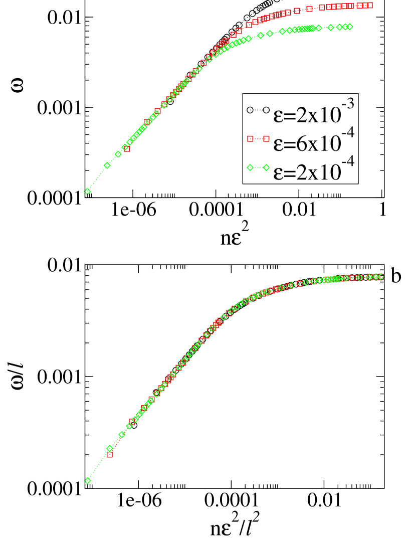
Figure 3: (a) Roughness evolution for different values of the control parameter $\epsilon$. (b) Collapse of the curves from (a) onto a universal curve. Both (a) and (b) were obtained using $V_{0}\approx 0$.

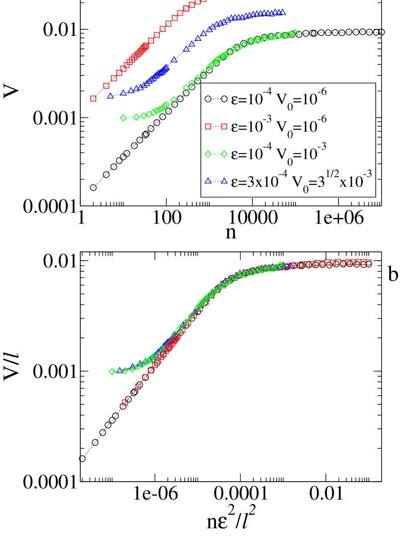
Figure 4: Behaviour of the average velocity $V$ as a function of $n$ for different values of $\epsilon$ and $V_{0}$. (a) The original time series. (b) Collapse of the data onto a universal curve.

We can also see that different values of the control parameter $\epsilon$ generate different behaviours for short $n$. This indicates that $n$ is not a scale variable. However, it turns out that the transformation $n\rightarrow n\epsilon^{2}$ coalesces the curves for small $n$ as illustrated in Fig. 1(b). We therefore infer: (i) that for $n\ll n_{x}$ the roughness grows according to

$$\omega(n\epsilon^{2},\epsilon,V_{0})\propto({n\epsilon^{2}})^{\beta}~{},$$ (4)

where exponent $\beta$ is called the growth exponent; (ii) that, as the iteration number increases, for $n\gg n_{x}$, the roughness reaches a saturation regime that is describable as

$$\omega_{\rm sat}(\epsilon)\propto\epsilon^{\alpha}~{},$$ (5)

where $\alpha$ is the roughening exponent; and (iii) that the crossover iteration number $n_{x}$ marking the approach to saturation is

$$n_{x}(\epsilon,V_{0})\propto\epsilon^{z}~{},$$ (6)

where $z$ is called the dynamical exponent. With these initial suppositions, we can now describe the roughness formally in terms of a scaling function,

$$\omega(n\epsilon^{2},\epsilon,V_{0})=l\omega(l^{a}n\epsilon^{2},l^{b}\epsilon,l^{c}V_{0})~{},$$ (7)

where $l$ is the scaling factor and $a$, $b$, and $c$ are referred to as scaling dimensions. It is important to stress that these scaling dimensions $a$, $b$ and $c$ must be related to the characteristic exponents $\alpha$, $\beta$ and $z$. All of the above discussion is also valid for the average velocity $V$. To relate the exponent $\beta$ to the scaling dimensions, we chose $l=(n\epsilon^{2})^{-{1\over{a}}}$. This allows us to rewrite (7) as

$$\omega(n\epsilon^{2},\epsilon,V_{0})=(n\epsilon^{2})^{-{1\over{a}}}\omega_{1}\left((n\epsilon^{2})^{-{b\over{a}}}\epsilon,(n\epsilon^{2})^{-{c\over{a}}}V_{0}\right)~{}.$$ (8)

The function $\omega_{1}=\omega\left(1,(n\epsilon^{2})^{-{b\over{a}}}\epsilon,(n\epsilon^{2})^{-{c\over{a}}}V_{0}\right)$ is supposed constant for $n\ll n_{x}$. Comparing equations (8) and (4), we can however conclude that $-{1\over{a}}=\beta$. Choosing $l=\epsilon^{-{1\over{b}}}$, we have that

$$\omega(n\epsilon^{2},\epsilon,V_{0})=\epsilon^{-{1\over{b}}}\omega_{2}\left((n\epsilon^{2})\epsilon^{-{a\over{b}}},\epsilon^{-{c\over{b}}}V_{0}\right)~{},$$ (9)

where $\omega_{2}=\omega\left((n\epsilon^{2})\epsilon^{-{a\over{b}}},1,\epsilon^{-{c\over{b}}}V_{0}\right)$ is assumed constant for $n\gg n_{x}$. Comparison of equations (9) and (5) shows that $-{1\over{b}}=\alpha$. It is less straightforward to obtain the exponent $c$. To do so, we use a result from a recent paper where two of us ref23 utilised a connection with the well known Standard Model (SM) ref3 to describe the position of the first invariant spanning curve (FISC) above the chaotic sea in the FUM. It was shown that the control parameter $\epsilon$ could be related to a typical mean velocity on the FISC in the FUM to give an effective control parameter $K_{\rm eff}=4\epsilon/{V^{*}}^{2}\approx 0.97\ldots$ which is gratifyingly close to the value of the control parameter $K_{\rm c}=0.9716\ldots$ at which the SM exhibits a transition from local to globally stochastic behaviour ref24 . We can thus rewrite the effective control parameter $K_{\rm eff}$ in terms of scaled variables as

$$K_{\rm eff}={4(l^{b}\epsilon)\over{(l^{c}V_{0})^{2}}}={4\epsilon\over{V_{0}^{2}}}{l^{b}\over{l^{2c}}}~{}.$$ (10)

which implies that $b-2c=0$. Using our result for the exponent $b$, we find $c=-{1\over{2\alpha}}$. Note that all scaling dimensions are therefore determined if we can obtain the exponents $\alpha$ and $\beta$ numerically. The exponent $\alpha$ is obtained in the asymptotic limit of large iteration number and it is independent of $V_{0}$. Fig. 2(a) illustrates an attempt to characterise this exponent using the extrapolated saturation roughness. Extrapolation is required because, even after $10^{3}n_{x}$ iterations, the roughness has still not quite reached saturation. From a power law fit, we obtain $\alpha=0.512(3)\approx 1/2$. We can thus rewrite Eq. (7) as

$$\omega(n\epsilon^{2},\epsilon,V_{0})=(n\epsilon^{2})^{\beta}g\left[(n\epsilon^{2})^{-2\beta}\epsilon,(n\epsilon^{2})^{-\beta}V_{0}\right]~{}.$$ (11)

In order to obtain $\beta$, we observe that we have two “time” scales in equation (11), namely $n_{x}^{\prime}$ and $n_{x}^{\prime\prime}$ and that the second one ($n_{x}^{\prime\prime}$) is basically zero if we chose $V_{0}\approx 0$. Then we determine $\beta$ from the short “time” behaviour ($n\ll n_{x}^{\prime}$). After averaging over different values of the control parameter $\epsilon$ in the range $\epsilon\in[10^{-4},10^{-1}]$, we then obtain $\beta=0.496(6)\approx 1/2$. Therefore, the scaling dimensions describing the scaling of the chaotic sea in the limit of small $\epsilon$ are $a=b=-2$ and $c=-1$. From Eqs. (6) and (8) we find that the scaling relation for the exponent $z$ is $z=\alpha/\beta-2$. Considering the previous values of both $\alpha$ and $\beta$, we obtain that $z=-1$. The exponent $z$ can be also obtained numerically. Fig. 2(b) shows the behaviour of the crossover iteration number $n_{x}$ as function of the control parameter $\epsilon$. The power law fit gives us that $z=-1.01(2)$, in good accord with the scaling result. The scaling for $V_{0}\approx 0$ is demonstrated in Fig. 3, where the three different curves for the roughness in (a) are very well collapsed onto the universal curve seen in (b) when we normalise the quantities with $a=b=-2$.

The case with initial velocity $V_{0}\neq 0$ is better illustrated by the average velocity (see Fig. 4). Now, we must consider two “time” scales, namely $n_{x}^{\prime}\propto 1/\epsilon$ and $n_{x}^{\prime\prime}\propto V_{0}^{2}/\epsilon^{2}$. From equation (10) (see also Ref. ref23 ), the maximum initial velocity inside the chaotic sea is $V_{0,{\rm max}}\approx 2\epsilon^{1/2}$ implying that the second time scale has a maximum value of ($n_{x}^{\prime\prime}\sim 4n_{x}^{\prime}$). So we observe that two different kinds of behaviour may occur, for $n_{x}^{\prime\prime}<n_{x}^{\prime}$ or $n_{x}^{\prime\prime}\sim n_{x}^{\prime}$. When $V_{0}=10^{-6}$, we have $n_{x}^{\prime\prime}\approx 0$ and we can see in Fig. 4(a) that the curves for $\epsilon=10^{-4}$ and $\epsilon=10^{-3}$ show only two regimes: (1) a growth in power law for $n\ll n_{x}^{\prime}$ and (2) the saturation regime for $n\gg n_{x}^{\prime}$. Considering $V_{0}=10^{-3}$ and $\epsilon=10^{-4}$ we have that $n_{x}^{\prime\prime}<n_{x}^{\prime}$ and we can see for such curve in Fig. 4(a) three regimes. For $n\ll n_{x}^{\prime\prime}$, the average velocity is basically constant. When $n_{x}^{\prime\prime}<n<n_{x}^{\prime}$, the curve growth and begin to follow the curve of $V_{0}=10^{-6}$ and same $\epsilon$. In this window of $n$, we have a growth with a smaller effective exponent $\beta$. Finally, for $n\gg n_{x}^{\prime}$ we have the saturation regime. It is shown in Fig 4(b) that the collapse of the curves holds even for $V_{0}\not=0$, implying that the inferred scaling form $V(n\epsilon^{2},\epsilon,V_{0})$ with exponents $a=b=-2$ and $c=-1$ is also correct.

In summary, we have characterised the average velocity and its variance (roughness) in the chaotic sea in the simplified FUM by use of a scaling function. We show that the critical exponents $\beta$, $\alpha$ and $z$ are connected by a scaling relation. We emphasise that this behaviour is valid for small values of $\epsilon$ and it is immediately extendable to other average quantities. We have characterised, for the first time, the scaling appearing in the integrability$\rightarrow$chaos transition (from $\epsilon=0$ to $\epsilon\not=0$) of the FUM. The scaling scenario should also hold for billiard systems, so that this kind of formalism should be useful for characterising asymptotic properties in such problems. It should be possible to extend it to encompass time-dependent Hamiltonian systems and a huge class of other problems exhibiting chaotic behaviour.

E. D. Leonel was supported by Conselho Nacional de Desenvolvimento Científico CNPq, from Brazil. The numerical results were obtained in the Centre for High Performance Computing in Lancaster University. The work was supported in part by the Engineering and Physical Sciences Research Council (UK). J. K. L. da Silva thanks to Conselho Nacional de Desenvolvimento Científico (CNPq) and Fundação de Amparo a Pesquisa de Minas Gerais (Fapemig), Brazilian agencies.

References

- (1) E. Fermi, Phys. Rev. 75, 1169 (1949).
- (2) A. J. Lichtenberg, M.A. Lieberman. Regular and Chaotic Dynamics(Appl. Math. Sci. 38, Springer Verlag, New York, 1992).
- (3) M.A. Lieberman and A. J. Lichtenberg. Phys. Rev. A 5, 1852 (1971).
- (4) L. D. Pustilnikov, Theor. Math. Phys. 57, 1035 (1983); L. D. Pustilnikov, Sov. Math. Dokl. 35(1), 88 (1987); L. D. Pustilnikov, Russ. Acad. Sci. Sb. Math. 82(1), 231 (1995).
- (5) A. J. Lichtenberg, M.A. Lieberman and R. H. Cohen Physica D 1, 291 (1980).
- (6) G. Karner, J. Stat. Phys. 77, 867 (1994).
- (7) S. T. Dembinski, A. J. Makowski and P. Peplowski, Phys. Rev. Lett. 70, 1093 (1993).
- (8) J. V. José and R. Cordery, Phys. Rev. Lett. 56, 290 (1986).
- (9) Z. J. Kowalik, M. Franaszek and P. Pieranski, Phys. Rev. A 37, 4016 (1988).
- (10) S. Warr, W. Cooke, R. C. Ball and J. M. Huntley, Physica A 231, 551 (1996).
- (11) N. Saitô, H. Hirooka, J. Ford, F. Vivaldi and G. H. Walker, Physica D 5, 273 (1982).
- (12) E. Canale, R. Markarian, S. O. Kamphorst and S. P. de Carvalho, Physica D 115, 189 (1998).
- (13) A. Loskutov, A. B. Ryabov and L. G. Akinshin, J. Phys. A: Math. Gen. 33, 7973 (2000).
- (14) A. -L. Barabási, H. E. Stanley, Fractal Concepts in Surface Growth (Cambridge University Press, Cambridge, 1985).
- (15) J. L. Mateos and J. V. José, Physica A 257, 434 (1998).
- (16) J. L. Mateos, Phys. Lett. A 256, 113 (1999).
- (17) G. A. Luna-Acosta, G. Orellana-Rivadeneyra, A. Mendoza-Galván and C. Jung, Chaos, Solitons and Fractals 12, 349 (2001).
- (18) E. D. Leonel and J. K. L. da Silva, Physica A 323, 181 (2003).
- (19) M. V. Berry, Eur. J. Phys. 2, 91 (1981).
- (20) M. Robnik and M. V. Berry, J. Phys. A 18, 1361 (1985).
- (21) The simplified FUM was introduced by Lichtenberg and Lieberman and can be found e.g. in Ref. ref3 .
- (22) E. D. Leonel, J. K. L. da Silva and S. O. Kamphorst, Physica A 331, 435 (2004).
- (23) We have used the same notation as the original work ref3 although, at that time, stochasticity was frequently referred as to chaotic behaviour. However we stress that the transition is from locally to globally chaotic behaviour. In the FUM, we mean by locally that the chaotic behaviour is confined by two different invariant spanning curves.