Semi-classical analysis of real atomic spectra beyond Gutzwiller’s approximation

Abstract

Real atomic systems, like the hydrogen atom in a magnetic field or the helium atom, whose classical dynamics are chaotic, generally present both discrete and continuous symmetries. In this letter, we explain how these properties must be taken into account in order to obtain the proper (i.e. symmetry projected) $\hbar$ expansion of semiclassical expressions like the Gutzwiller trace formula. In the case of the hydrogen atom in a magnetic field, we shed light on the excellent agreement between present theory and exact quantum results.

In the studies of the quantum properties of systems whose classical counterparts depict chaotic behavior, semi-classical formulas are essential links between the two worlds, emphasized by Gutzwiller’s work Gutzwiller90 . More specifically, starting from Feynman’s path formulation of quantum mechanics, he has been able to express the quantum density of states as a sum over all (isolated) periodic orbits of the classical dynamics. This formula, and extensions of it, have been widely used to understand and obtain properties of the energy levels of many classically chaotic systems, among which the hydrogen atom in a magnetic field FW89 ; Houches89 , the helium atom Ezra91 ; GR93 ; GG98 or billiards Bu79 ; CE89 ; GA93 ; GAB95 .

At the same time, because the trace formula (and its variations) as derived by Gutzwiller only contained the leading term of the asymptotic expansion of the quantum level density, the systematic expansion of the semiclassical propagator in powers of $\hbar$ has been the purpose of several studies GA93 ; GAB95 ; VR96 ; WMW02 , but which focused on billiards, for which both classical and quantum properties are easier to calculate.

In a recent paper pre65G , general equations for efficient computation of $\hbar$ corrections in semi-classical formulas for a chaotic system with smooth dynamics were presented, together with explicit calculations for the hydrogen atom in a magnetic field. However, only the two-dimensional case was considered, because for the three-dimensional (3D) case, discrete symmetries and centrifugal terms had to be taken into account. Actually, this situation occurs in almost all real atomic systems depicting a chaotic behavior (molecules, two electron atoms…), for which experimental data involve levels having well defined parity, total angular momentum and, if relevant, exchange between particles. In particular, semi-classical estimations of experimental signals like photoionization cross-sections are calculated with closed orbits with vanishing total angular momentum, whereas they usually involve $P$ ($L=1$) quantum states, whose positions in energy are shifted with respect to $S$ ($L=0$) states. Furthermore, in recent years, the development of the harmonic inversion method makes it possible to extract the relevant quantities (position of peaks, complex amplitudes) from both theoretical and experimental data with a much higher accuracy than with the conventional Fourier transform M99 . In particular, it becomes possible to measure the deviation of the exact quantum results from the semi-classical leading order predictions. Thus, a detailed semi-classical analysis of experimental results, beyond the leading order in $\hbar$, requires the understanding and the calculation of corrections due to both the discrete symmetries and centrifugal terms. In addition, we would like to stress that even if the present analysis is made with the density of states, it can also be made with the Quantum Green function, which leads to expressions and numerical computations of the first order $\hbar$ corrections for physical quantities like the photo-ionization cross-section B89 ; GD92 , which could either be compared to available experimental data Holle88 ; Main94 , or become a starting point for refined experimental tests of the quantum-classical correspondence in the chaotic regime.

$\hbar$ corrections and discrete symmetries have already been discussed, but only for billiards GA93 ; GAB95 ; WMW02 , whereas in the case of systems with smooth dynamics a detailed study is still lacking. Also, centrifugal terms and/or rotational symmetries have been considered by many authors, but either in the case of integrable systems schulman ; KL75 , or for values of the angular momentum comparable to the action of classical orbits Gutzwiller90 ; praCL44 ; jpaCL25 . From this point of view, the present study, which focuses on fixed values of the quantum angular momentum and the effect of the centrifugal terms on $\hbar$ corrections for systems with smooth chaotic dynamics, goes beyond the preceding considerations. More precisely, in this letter, we explain how to take into account both discrete symmetries and centrifugal terms in order to obtain a full semi-classical description of the first order $\hbar$ corrections for the 3D hydrogen atom in a magnetic field.

At first, in the case of a chaotic system, whose Hamiltonian $H=\mathbf{p}^{2}/2+V(\mathbf{q})$ is invariant under a group $\mathcal{S}$ of discrete transformations $\sigma$, the leading order of semi-classical approximation for the trace of the Green function $G(E)=1/(E-H)$, restricted to the $m^{\mathrm{th}}$ irreducible representation is given by pra40R :

$$g_{m}^{\mathrm{sc}}(E)=\frac{d_{m}}{i\hbar}\sum_{l}\frac{T_{l}}{|K_{l}|}\sum_{n}\chi_{m}(\sigma_{l}^{n})g_{(l,n)}^{(0)}(E)$$ (1)

with

$$g_{(l,n)}^{(0)}(E)=\frac{1}{|\det{(A^{n}_{l}-\openone)}|^{1/2}}\exp{\left[\frac{i}{\hbar}nS_{l}-in\mu_{l}\frac{\pi}{2}\right]}$$ (2)

where the $l$ sum is taken over all primitive (isolated) orbits which become periodic through the symmetry operation $\sigma_{l}$ (i.e. final position (resp. velocity) is mapped back to initial position (resp. velocity) by $\sigma_{l}$). $\chi_{m}(\sigma_{l}^{n})$ is the character of $\sigma_{l}^{n}$ in the $m^{\text{th}}$ irreducible representation of dimension $d_{m}$. $S_{l}$ is the action of the orbit $l$, $\mu_{l}$ the Maslov index, $T_{l}$ the “period”, $A^{n}_{l}$ represents the Poincaré surface-of-section map linearized around the orbit and $K_{l}$ is the subgroup of $\mathcal{S}$ leaving each point of the orbit $l$ invariant. Adding first order $\hbar$ corrections, the preceding equation (1) becomes :

$$g_{m}^{\mathrm{sc}}(E)=\frac{d_{m}}{i\hbar}\sum_{l}\frac{T_{l}}{|K_{l}|}\sum_{n}\chi_{m}(\sigma_{l}^{n})g_{(l,n)}^{(0)}(E)\biggl{(}1+i\hbar\mathcal{C}_{(l,n)}^{\mathrm{tr}}\biggr{)}$$ (3)

$\mathcal{C}_{l,n}^{\mathrm{tr}}$ can be derived by a detailed analysis of the stationary phase approximations starting from the Feynman path integral, following the same steps as in Ref. GAB95 ; pre65G and reads as follows :

$$\mathcal{C}_{l,n}^{\mathrm{tr}}=C_{l,n}^{T\rightarrow E}+\frac{1}{nT_{l}}\int_{0}^{nT_{l}}\!dt_{0}\,C_{l,n}(t_{0})$$ (4)

where $C_{l,n}^{T\rightarrow E}$ arises from the time to energy domain transformation. $C_{l,n}(t_{0})$ (see Ref. pre65G for the expressions) involves the classical Green functions $\mathcal{G}_{l,n}(t,t^{\prime})$, i.e. the solutions of the equations controlling the linear stability around the classical trajectory $\mathbf{q}^{\mathrm{cl}}_{l,n}(t)$ :

$$\biggl{(}-\frac{\mathrm{d}^{2}}{\mathrm{d}t^{2}}\openone-\frac{\partial^{2}V}{\partial\mathbf{q}\partial\mathbf{q}}\left[\mathbf{q}^{\mathrm{cl}}_{l,n}(t)\right]\biggr{)}\mathcal{G}_{l,n}(t,t^{\prime})=\openone\,\delta(t-t^{\prime}).$$ (5)

The fact that the orbits are periodic after the symmetry transformation $\sigma_{l}^{n}$ determines the boundary conditions that the classical Green functions $\mathcal{G}_{l,n}(t,t^{\prime})$ must fulfill, namely :

$$\left\{\begin{aligned} \sigma_{l}^{-n}\mathcal{G}_{l,n}(nT_{l},t^{\prime})&=\mathcal{G}_{l,n}(0,t^{\prime})\\ \mathcal{P}_{t_{0}}\mathcal{G}_{l,n}(0,t^{\prime})&=0\\ \mathcal{Q}_{t_{0}}\sigma_{l}^{-n}\dot{\mathcal{G}}_{l,n}(nT_{l},t^{\prime})&=\mathcal{Q}_{t_{0}}\dot{\mathcal{G}}_{l,n}(0,t^{\prime})\end{aligned}\right.\qquad\forall t^{\prime}\in[0,nT_{l}]$$ (6)

where $\mathcal{P}_{t_{0}}$ is the projector along the “periodic” orbit at the position depicted by time $t_{0}$ and $\mathcal{Q}_{t_{0}}=\openone-\mathcal{P}_{t_{0}}$. Of course, for $\sigma_{l}=\openone$, one recovers the boundary conditions given in Ref. pre65G . Finally, all technical steps of Ref. pre65G leading to efficient computation of $\mathcal{G}_{l,n}(t,t^{\prime})$ and $\hbar$ corrections, that is, solutions of sets of first order differential equations, can easily be adapted to take into account these modified boundary conditions.

As a numerical example, we have considered the 2D hydrogen atom in a magnetic field, at scaled energy $\epsilon=-0.1$ FW89 . More precisely, we have computed the trace of the quantum Green function, using roughly 8000 states belonging to the $EEE$ representation MWR89 of the group $D_{4}$, corresponding to effective $1/\hbar$ values ranging from $0$ to $124$ (See Ref. pre65G for further details). In that case, the periodic orbit $\overline{1234}$ EW90 ; H95 (see inset of the top of Fig. 1 for the trajectory in semi-parabolic coordinates), being (globally) invariant under a rotation of angle $\pi/2$, gives rise to contributions in the semi-classical approximation of the trace at all multiples of $S_{\overline{1234}}/4$. In the same way, the periodic orbit $\overline{1243}$ (see middle inset of Fig. 1) being invariant under a rotation of angle $\pi$, contributions are present at all multiples of $S_{\overline{1243}}/2$. For both these orbits, table 1 displays the comparison of the present theoretical calculation and the numerical coefficient $\mathcal{C}_{l,n}^{HI}$, extracted from the exact quantum Green function, using harmonic inversion M99 ; pre65G . As one can notice, the agreement is excellent for the amplitudes and rather good for the phases, which is the usual behavior of harmonic inversion. Furthermore, the same agreement has also been found for the other representations, thus emphasizing the present approach for the calculation of the first order $\hbar$ corrections when taking into account discrete symmetries.

Table 1: Numerical comparison between the theoretical $\hbar$ corrections $\mathcal{C}_{l}^{\mathrm{tr}}$ for the trace of the quantum Green function, restricted to the $EEE$ representation, of the 2D hydrogen atom in a magnetic field and the numerical coefficients $\mathcal{C}_{l}^{HI}$ extracted from exact quantum function using harmonic inversion. The agreement is excellent for the amplitudes and rather good on the phases, thus emphasizing the validity of the present approach.

Code	$\mathcal{C}_{l}^{\mathrm{tr}}$	$|\mathcal{C}_{l}^{HI}|$	Rel. error	$\arg{\mathcal{C}_{l}^{HI}}$
$\frac{1}{4}\overline{1234}$	$-$0.094 430	0.09445	$\approx 2\times 10^{-4}$	0.9996$\times\pi$
$\frac{1}{2}\overline{1234}$	$-$0.361 689	0.3611	$\approx 2\times 10^{-3}$	0.996$\times\pi$
$\frac{3}{4}\overline{1234}$	$-$0.400 555	0.3992	$\approx 3\times 10^{-3}$	1.005$\times\pi$
$\frac{1}{2}\overline{1243}$	0.049 339	0.0493	$\approx 8\times 10^{-4}$	-0.075$\times\pi$

Contrary to the preceding, calculating first order $\hbar$ corrections due to centrifugal terms is more complicated and is best explained in the case of the 3D hydrogen atom in a magnetic field. The regularized Hamiltonian in semiparabolic coordinates, for fixed value $M$ of the projection of the angular momentum along the field axis, is given by FW89  :

$$H =-\frac{\hbar^{2}}{2}\left(\frac{\partial^{2}}{\partial u^{2}}+\frac{\partial^{2}}{\partial v^{2}}+(\frac{1}{4}-|M|^{2})\left[\frac{1}{u^{2}}+\frac{1}{v^{2}}\right]\right)$$ (7)

$$\qquad\qquad\qquad-\epsilon(u^{2}+v^{2})+\frac{1}{8}u^{2}v^{2}(u^{2}+v^{2})$$

$$=H_{0}+\frac{\hbar^{2}}{2}\left(|M|^{2}-\frac{1}{4}\right)U(u,v).$$

$H_{0}$ is then the Hamiltonian of the 2D hydrogen atom in a magnetic field. If $U(u,v)$ was regular, then the additional first order $\hbar$ correction for the orbit $l$ would simply be :

$$-\frac{1}{2}\left(|M|^{2}-\frac{1}{4}\right)\int_{0}^{T_{l}}\!dt\,U(u_{l}(t),v_{l}(t)).$$ (8)

One must mention that in this case, the Langer transformation L37 of the coordinates $(u,v)\rightarrow(\exp{(-x)},\exp{(-y)})$ gives rise to a Hamiltonian which does not separate into kinetic and potential energies and for which no expressions for $\hbar$ corrections are available.

On the other hand, the fact that $U(u,v)$ is singular imposes boundary conditions on both classical and quantum dynamics. The classical trajectories have to make (smooth) bounces near $u=0$ and $v=0$ and for vanishing values of $\hbar$, we expect the trajectories of $H$ to be those of $H_{0}$, but mapped onto the reduced phase space $(u>0,v>0)$, i.e. making hard bounces on the $(u,v)$ axis. From the quantum point of view, depending on the parity of $M$, only wavefunctions belonging to given representations of $D_{4}$ are allowed. Thus, first order $\hbar$ corrections due to the singular part of the potential $U$, are given by the preceding considerations on the symmetries, whereas remaining corrections are given by Eq. (8), where $U$ has to be replaced by a smooth counterpart, namely :

$$\tilde{U}=\lim_{\epsilon\rightarrow 0^{+}}\frac{1}{2}\left(\frac{1}{(u+i\epsilon)^{2}}+\frac{1}{(u-i\epsilon)^{2}}+\frac{1}{(v+i\epsilon)^{2}}+\frac{1}{(v-i\epsilon)^{2}}\right).$$ (9)

Actually, one can show that the preceding equation gives the right answers for $\hbar$ expansion of the propagator of the free particle (up to $\hbar^{3}$) and the harmonic oscillator (up to $\hbar^{2}$), for which analytical expressions for classical trajectories, classical Green functions and quantum propagators exist (higher orders have not been checked yet). However, even if a detailed analysis of the derivation of the trace formula in presence of centrifugal terms seems to show that the preceding approach works in general cases, rigorous proof of Eq. (9) is lacking.

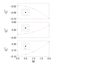
Figure 1: First order $\hbar$ correction to the semi-classical approximation of the trace of the quantum Green function for the hydrogen atom in a magnetic field for different values of the magnetic number $M$, $M=1/2$ corresponding to the 2D case pre65G . Crosses depict the values extracted from the exact quantum function using harmonic inversion, whereas the solid line corresponds to the classical results given by Eq. (10). For the three different periodic orbits, whose trajectories in the $(u,v)$ plane are plotted (the nucleus being depicted by the black dot), the agreement is excellent, thus emphasizing the validity of Eq. (9) and Eq. (10).

Nevertheless, in the case of the 3D hydrogen atom in a magnetic field, we have compared the first order $\hbar$ corrections, for different periodic orbits and for different values of the magnetic number $M$, with the present prediction, namely :

$$C_{l}^{\mathrm{tr}}(M)=C_{l}^{\mathrm{tr}}(2D)-\frac{1}{8}\left(4|M|^{2}-1\right)\int_{0}^{T_{l}}\!dt\,\tilde{U}(u_{l}(t),v_{l}(t)).$$ (10)

The results are displayed in Fig. 1 for $M=0,1,2$ and for three different orbits, namely $\overline{1234}$, $\overline{1243}$ and $\overline{12343}$, whose trajectories in the $(u,v)$ plane are plotted. The solid line is the theoretical result given by Eq. (10), whereas the crosses are the values extracted from the trace of the exact quantum Green function, using harmonic inversion (for scaled energy $\epsilon=-0.1$, roughly 8000 effective $1/\hbar$ values ranging from $0$ to $124$). As one can notice the agreement is excellent, thus giving strong support for the validity of Eq. (9) and Eq. (10). Furthermore, the simplicity of the replacement $\tilde{U}$ may serve as a guideline for a rigorous treatment of the $\hbar$ corrections arising from the centrifugal terms. In particular, the calculation of higher orders involves products of the derivatives of these centrifugal terms and those of the potential $V_{0}$, giving rise to non-trivial mixing between centrifugal and standard $\hbar$ corrections.

In conclusion, we have presented a semi-classical analysis, beyond the usual Gutzwiller approximation, including first order $\hbar$ corrections, of the quantum properties of real chaotic systems. More specifically, we have explained the additional corrections arising when taking into account both discrete symmetries and centrifugal terms. In the case of the (3D) hydrogen in a magnetic field, the agreement between the theory and the numerical data extracted from exact quantum results is excellent, emphasizing the validity of the analysis, especially of equations (9) and (10).

Finally, since we know how to compute the $\hbar$ corrections, it would be very interesting to work the other way round, that is, to perform the semi-classical quantization, thus getting $\hbar$ corrections in the semi-classical estimations of the quantum quantities, like the eigenenergies. Of course, this represents a more considerable amount of work, since the $C_{l,n}^{\mathrm{tr}}$ coefficients must be computed for all relevant orbits and then included in standard semi-classical quantization schemes, like the cycle expansion EC89 ; GR93 ; VR96 .

- (1) Chaos in Classical and Quantum Mechanics, M.C. Gutzwiller (Springer, New York, 1990).
- (2) H. Friedrich and D. Wintgen, Phys. Rep. 183, 37 (1989).
- (3) D. Delande, in Chaos and Quantum Physics, edited by M.-J. Giannoni, A. Voros, and J. Zinn-Justin, Les Houches Summer School, Session LII (North-Holland, Amsterdam, 1991).
- (4) G.S. Ezra, K. Richter, G. Tanner, and D. Wintgen, J. Phys. B 24, L413 (1991).
- (5) P. Gaspard and S.A. Rice. Phys. Rev. A 48, 54 (1993).
- (6) B. Grémaud and P. Gaspard, J. Phys. B 31, 1671 (1998).
- (7) L.A. Bunimovitch, Commun. Math. Phys. 65, 295 (1979).
- (8) P. Cvitanović and B. Eckhardt, Phys. Rev. Lett. 63, 823 (1989).
- (9) P. Gaspard and D. Alonso, Phys. Rev. A 47, R3468 (1993).
- (10) P. Gaspard, D. Alonso, and I. Burghardt, Adv. Chem. Phys. XC 105 (1995).
- (11) G. Vattay and P. E. Rosenqvist, Phys. Rev. Lett. 76, 335 (1996).
- (12) K. Weibert, J. Main, G. Wunner, Eur. Phys. J. D 19, 379 (2002).
- (13) B. Grémaud, Phys. Rev. E 65, 056207 (2002).
- (14) J. Main, Phys. Rep. 316, 233 (1999).
- (15) E. P. Bogomolny, Zh. Eksp. Teor. Fiz. 96, 487 (1989) [Sov. Phys. JETP 69, 275 (1989)].
- (16) J. Gao and J. B. Delos, Phys. Rev. A 46, 1455 (1992).
- (17) A. Holle, J. Main, G. Wiebusch, H. Rottke, and K. H. Welge, Phys. Rev. Lett. 61, 161 (1988).
- (18) J. Main, G. Wiebusch, K. Welge, J. Shaw, and J. B. Delos, Phys. Rev. A 49, 847 (1994).
- (19) Techniques and Applications of Path Integration, L.S. Schulmann, (J. Wiley, New-York, 1981).
- (20) K.C. Khandekar and S.V. Lawande, J. Math. Phys. 16, 384 (1975).
- (21) S.C. Creagh and R. G. Littlejohn, Phys. Rev. A 44, 836 (1991)
- (22) S.C. Creagh and R. G. Littlejohn, J. Phys. A 25, 1643 (1992)
- (23) J. M. Robbins, Phys. Rev. A 40, 2128 (1989).
- (24) C. C. Martens, R. L. Waterland, and W. P. Reinhardt, J. Chem. Phys. 90, 2328 (1989).
- (25) B. Eckhardt and D. Wintgen, J. Phys. B 23, 355 (1990).
- (26) K. T. Hansen, Phys. Rev. E 51, 1838 (1995).
- (27) R.E. Langer, Phys. Rev. 51, 669 (1937)
- (28) P. Cvitanović and B. Eckhardt, Phys. Rev. Lett. 63, 823 (1989)