Awaking and Sleeping a Complex Network

Abstract

A network with local dynamics of logistic type is considered. We implement a mean-field multiplicative coupling among first-neighbor nodes. When the coupling parameter is small the dynamics is dissipated and there is no activity: the network is turned off. For a critical value of the coupling a non-null stable synchronized state, which represents a turned on network, emerges. This global bifurcation is independent of the network topology. We characterize the bistability of the system by studying how to perform the transition, which now is topology dependent, from the active state to that with no activity, for the particular case of a scale free network. This could be a naive model for the wakening and sleeping of a brain-like system.

Keywords: Complex networks, neuronal models, brain-like systems, logistic coupling, bistability.
PACS numbers: 89.75.Hc, 89.75.Fb, 87.19.La
Electronic mails: ^‡ rilopez@unizar.es ; ^† yamir@unizar.es, amalio@unizar.es ; ^§ stefano@ino.it, duhwang@ino.it

1 Introduction

Understanding the brain is a formidable challenge. A multidisciplinary effort is required to enlighten how it works, how it processes information and how it takes decisions. Furthermore, the brain behaviors which are considered far from those commonly accepted, that is, the mental illnesses or the degenerative cerebral evolutions, are important problems that are under constant investigation. The different approaches from the most diverse fields, i.e., medicine, psychiatry, neurobiology, chemistry and neural computation, should combine their particular visions for trying to reach the collective goal of creating an artificial brain-like system or, at least, in order to reach solutions to the most diverse dysfunction symptoms which are found in its behavior.

Different models have been proposed to catch the computational principles of mental processes. Neural networks are considered as a paradigmatic model alternative to the more traditional models such as finite automata, Turing machines and Boolean circuits. In fact, neural nets have an inspiration more grounded in the neurophysiological structure of the neuronal system. A survey of the underlying results concerning the computational power and complexity issues of neuronal network models can be found in (Sima, & Orponen, 2003) and references therein.

In a certain sense and from a physical point of view, brain can be considered as a clock controlled by the internal circadian rhythm. Hence, it is synchronized with the day/night cycle (Winfree, 1986). Roughly speaking, two states can be associated with this cycle: awake and sleep. This property is universally observed in all animals. The cerebral activity is dissociated from the sensory and motor neurons in the sleep state. This dissociation is not complete and the brain can still respond to some sensory stimuli. In fact there are qualitatively different patterns of neural activity between different stages of sleep. Basically, two levels, a deepest one and a shallowest one, alternate during the sleep. The deepest level of sleep is attained rapidly and, as sleep progresses, the average level becomes shallower. The substances that control the connection among neurons or synopsis monitor theses changes in the neural activity, which is formed out of composite states occurring in disconnected brain subdivisions. When the full connections are restablished, the waking state of the brain is recovered (Bar-Yam, 1997).

So, as it is suggested by real measurements of the electrical brain activity, synchrony seems to be a key concept to explain different aspects of neuronal behavior. The activities of two or more neurons, which we call a functional unit, are said to be synchronized when some kind of temporal correlations exists among them. The conditions for the emergence of these states are a central issue in the research of neuronal activity (Borgers, & Kopell, 2003; Hansel, & Mato, 2003). It has been recently argued (Eguiluz, Chialvo, Cecchi, Baliki, & Apkarian, 2003) that the distribution of functional connections in the human brain follows the same distribution of a scale-free network. This finding means that there are regions in the brain that participate in a large number of tasks while most of the other functional units are only involved in a tiny fraction of the brain’s activities. The previous network adds to many examples of such a distribution found in the last few years in fields as diverse as biological, technological and social systems (Strogatz, 2001; Dorogovtsev, & Mendes, 2003; Bornholdt, & Schuster, 2002; Pastor-Satorras, & Vespignani, 2004). They have been termed scale-free networks because the probability of finding an element with $k$ connections to other elements of the network follows a power-law $P(k)\sim k^{-\gamma}$, where $\gamma$ usually lies between $2$ and $3$.

In this work we propose a naive approach to mimic the brain bistability between the sleep and the awake states, and to explain how to perform the transition between those two basic configurations, namely the switched on and the switched off states. In section 2, a model for a general network showing bistability is proposed and analyzed. In section 3, the transition between the active and the non active states is studied. As our model is thought of as a system made up of functional units and they seem to be distributed according to a power law, we focus our attention in the on-off transition for the case of a random scale-free network. The last section contains our discussion and conclusions.

2 The Model

Brain is a complex network. Millions of neurons are unidirectionally and locally interconnected there. In a first and simple approach one can consider a functional unit, i.e. a neuron or group of neurons (in the following, neuron or functional unit are used indistinctly), as a discrete dynamical system with two possible states: one active state and another one with no activity. Let $x_{n}^{i}$ be, with $0<x_{n}^{i}<1$, a measurement of the $ith$ network neuron activity at time $n$. Take, for instance, a logistic evolution (May, 1976) for the local neuronal activity:

$$x^{i}_{n+1}=\bar{p}\;x^{i}_{n}(1-x^{i}_{n}).$$ (1)

It presents only one stable state for each $\bar{p}$. For $\bar{p}<1$, the dynamics dissipates to zero, $x_{n}^{i}=0$, then it can represent the functional unit with no activity. For $1<\bar{p}<4$, the dynamics is non null and it would represent an active neuron. This local transition is controlled by the parameter $\bar{p}$. The functional dependence of this local coupling on the neighbor states is essential in order to get a good brain-like behavior of the network. It seems reasonable to take $\bar{p}$ as a linear function (that we call the Alesves coupling) depending on the actual mean value, $X_{n}^{i}$, of the neighboring signal activity and expanding the interval $(1,4)$ in the form:

$$\bar{p}=p\;(3X_{n}^{i}+1),$$ (2)

with

$$X_{n}^{i}={1\over N_{i}}\sum_{j=1}^{N_{i}}x_{n}^{j}.$$ (3)

$N_{i}$ is the number of neighbors of the $ith$ neuron, and $p$, which gives us an idea of the neuron interaction with its first-neighbor neurons, is the control parameter. This parameter runs in the range $0<p<p_{max}$, where $p_{max}\succeq 1$. Let us observe that there is an unrealistic bi-directionality in the local neuronal connectivity in this naive approach to brain-like systems. This is not a drawback since networks built under this insight show an interesting bistability which can mimic the brain behavior. Hence, they present an attractive global null configuration that will be identified as the turned off state of the network. Also they show a completely synchronized non-null stable configuration that we identify as the turned on state of the network. Thus, it is necessary a critical level of noise to transit from the turned off state to the turned on one for a given $p$. The different sleep states, including dreams in human brain, can be interpreted as a noisy neuronal activity which does not reach that critical value. The transition from the awake to the sleep state can be performed either by decreasing the coupling $p$ or by making zero the activity of some units. All these dynamical properties are universal for different kinds of local evolution of the same type as equation (1), the so-called unimodal maps.
Let us mention at this point that phase synchronization and cluster formation in coupled maps on different networks has been studied, for instance, in (Jalan & Amritkar, 2003). The results exposed in that work are very different from those here explained. Concretely, they find that perfect synchronization leads to clusters with very small number of nodes. On the contrary, a robust bistability between two perfect synchronized states is obtained in our system, as it is shown in the next sections.

2.1 Two-neuron system

Let us start with the simplest case of two interconnected functional units. The dynamics is given in this case by the coupled equations:

$$x^{1}_{n+1}=p\;(3x^{2}_{n}+1)\;x^{1}_{n}(1-x^{1}_{n}),$$ (4)

$$x^{2}_{n+1}=p\;(3x^{1}_{n}+1)\;x^{2}_{n}(1-x^{2}_{n}).$$ (5)

Depending on the coupling $p$ different dynamical regimes are obtained (see the details and nomenclature in references (Lopez-Ruiz, & Fournier-Prunaret, 2004; Lopez-Ruiz, & Fournier-Prunaret, 2003), $p_{max}=1.0843$ in this case):

• For $0<p<0.75$, the dynamics vanishes. The two-neuron network does not have long-term activity. The whole square $[0,1]\times[0,1]$ of initial conditions shrinks to the turned off configuration, that is, the fixed point $x_{\theta}=(0,0)$.

• For $0.75<p<0.86$, the synchronized state, $x_{+}=(\bar{x},\bar{x})$, with $\bar{x}={1\over 3}\{1+(4-{3\over p})^{1\over 2}\}$, which arises from a saddle-node bifurcation for the critical value $p_{0}=0.75$, is a stable turned on state. This state coexists with $x_{\theta}$. The system presents now bistability and depending on the initial conditions, the final state can be $x_{\theta}$ or $x_{+}$. Switching on the system from $x_{\theta}$ requires a level of noise in both neurons sufficient to render the activity on the basin of attraction of $x_{+}$. On the contrary, switching off the two-neuron network can be done, for instance, by making zero the activity of one neuron, or by doing the coupling $p$ lower than $p_{0}$.

• For $0.86<p<0.95$, the active state of the network is now a period-$2$ oscillation. This new dynamical state bifurcates from $x_{+}$ for $p=p_{c}=0.86$. A smaller noise is necessary to activate the system from $x_{\theta}$. Making zero the activity of one neuron continues to be a good strategy to turn off the network.

• For $0.95<p<1$, the active state acquires a new frequency and presents quasiperiodicity. It is still possible to switch off the network by putting to zero one of the neurons.

• For $1<p<1.03$, bistability is lost. When $p=p_{f}=1$ the turned off state $x_{\theta}$ loses stability and the only stable dynamical state for $p>p_{f}$ is now the turned on network. The network stores the information in a quasiperiodic state.

• For $1.03<p<1.08$, a more complex active state is obtained. In this range, the network can store more complicated information in the stable chaotic state, which is now present in the system.

• For $p>1.0843$, the network loses stability and it can not store information anymore.

Let us remark that the two-neuron system exhibits, from a qualitative point of view, the properties desirable for a brain-like system: bistability between an active state and another one with no activity in the range $p_{0}<p<p_{f}$ , a necessary noisy level to attain the activation of the network from the switch off state, and two different possible strategies to turn off the system from the active state, by decreasing the synaptic coupling under a critical value or by putting to zero one of the neurons.
We proceed now to show that those properties are still present in a general complex network.

2.2 Many neuron system

The complete synchronization (Boccaletti, Kurths, Osipov, Valladares, & Zhou, 2002) of the network means that $x_{n}^{i}=x_{n}$ for all $i$ , with $i=1,2,\ldots,N$ and $N\gg 1$. Hence, we also have $X_{n}^{i}=x_{n}$. The time evolution of the network on the synchronization manifold is then given by the cubic mapping:

$$x_{n+1}=p\;(3x_{n}+1)\;x_{n}(1-x_{n}).$$ (6)

The fixed points of this system are found by solving $x_{n+1}=x_{n}$. The solutions are $x_{\theta}=0$ and $x_{\pm}={1\over 3}\{1\pm(4-{3\over p})^{1\over 2}\}$. The first state $x_{\theta}$ is stable for $0<p<1$ and $x_{\pm}$ take birth after a saddle-node bifurcation for $p=p_{0}=0.75$. The node $x_{+}$ is stable for $0.75<p<1.157$ and the saddle $x_{-}$ is unstable. Therefore bistability between the states

$$x_{n}^{i}=x_{\theta}, \forall i\longrightarrow TURNED\;\;\;OFF\;\;\;STATE,$$ (7)

$$x_{n}^{i}=x_{+}, \forall i\longrightarrow TURNED\;\;\;ON\;\;\;STATE,$$ (8)

seems to be also possible for $p>p_{0}$ in the case of many interacting units. But stability in the synchronization manifold does not imply the global stability. Small transverse perturbations to this manifold can make unstable the synchronized states. Let us suppose then a general local perturbation $\delta x_{n}^{i}$ of the element activity,

$$x_{n}^{i}=x_{*}+\delta x_{n}^{i},$$ (9)

with $x_{*}$ representing a synchronized state. We define the perturbation of the local mean-field as

$$\delta X_{n}^{i}={3\over N_{i}}\sum_{j=1}^{N_{i}}\delta x_{n}^{j}.$$ (10)

If these expressions are introduced in equation (1), we find the time evolution of the local perturbations:

$$\delta x_{n+1}^{i}=p\,(3x_{*}+1)(1-2x_{*})\delta x_{n}^{i}+p\,x_{*}(1-x_{*})\delta X_{n}^{i}.$$ (11)

The dynamics for the local mean-field perturbation is derived by substituting this last expression in relation (10). We obtain:

$$\delta X_{n+1}^{i}=p\,(3x_{*}+1)(1-2x_{*})\delta X_{n}^{i}+3p\,x_{*}(1-x_{*}){1\over N_{i}}\sum_{j=1}^{N_{i}}\delta X_{n}^{j}.$$ (12)

We express now the local mean-field perturbations of the first-neighbors as function of the local mean-field perturbation $\delta X_{n}^{i}$ by defining the local operational quantity $\sigma_{i}^{n}$,

$${1\over N_{i}}\sum_{j=1}^{N_{i}}\delta X_{n}^{j}=\sigma_{n}^{i}\;\delta X_{n}^{i},$$ (13)

which is determined by the dynamics itself. If we put together the equations (11-12), the linear stability of the synchronized states holds as follows:

$$\left(\begin{array}[]{c}\delta x_{n+1}^{i}\\ \delta X_{n+1}^{i}\end{array}\right)=\left(\begin{array}[]{cc}p\,(3x_{*}+1)(1-2x_{*})&p\,x_{*}(1-x_{*})\\ 0&p\,(3x_{*}+1)(1-2x_{*})+3p\,\sigma_{n}^{i}\,x_{*}(1-x_{*})\end{array}\right)\left(\begin{array}[]{c}\delta x_{n}^{i}\\ \delta X_{n}^{i}\end{array}\right).$$ (14)

Let us observe that the only dependency on the network topology is included in the quantity $\sigma_{n}^{i}$. The rest of the stability matrix is the same for all the nodes and therefore it is independent of the local and global network organization.

The turned off state is $x_{*}=x_{\theta}=0$. The eigenvalues of the stability matrix are in this case $\lambda_{1}=\lambda_{2}=p$. Thus, this state is an attractive state in the interval $0<p<1$. It loses stability for $p=1$, then the highest value $p_{f}$ of the parameter $p$ where bistability is still possible satisfies $p_{f}\leq 1$.

The turned on state $x_{+}$ verifies $x_{*}=x_{+}={1\over 3}\{1+(4-{3\over p})^{1\over 2}\}$. If we suppose $\sigma_{n}^{i}=\sigma$, the eigenvalues of the stability matrix are $\lambda_{1}=2-2p-p(4-{3\over p})^{1\over 2}$ and $\lambda_{2}=\lambda_{1}+{\sigma\over 3}(3-2p+p(4-{3\over p})^{1\over 2})$. Let us observe that $\lambda_{1}=-1$ for $p=1$. This implies that the parameter $p_{c}$ for which the synchronized state $x_{+}$ looses stability verifies $p_{c}\leq 1$. Depending on the sign of $\sigma$, we can distinguish two cases in the behavior of $p_{c}$:

• If $0<\sigma<1$, we find that $\mid\lambda_{2}\mid<1$. Then $x_{+}$ bifurcates through a global flip bifurcation for $p=p_{c}=1$. In this case, the bifurcation of the synchronized state $x_{+}$ for $p_{c}=1$ coincides with the loss of the network bistability for $p_{f}=1$. Hence $p_{c}=p_{f}=1$ for this kind of networks, and the bistability holds between $x_{\theta}$ and $x_{+}$ in the parameter interval $p_{0}=0.75<p<p_{c}=p_{f}=1$. As an example, an all-to-all network shows this behavior because $\sigma=1$. This is represented in the inset of Fig. 1.

• If $-1<\sigma<0$, then $\lambda_{2}=-1$ is obtained for a $p=p_{c}$ smaller than $1$. Therefore it is now possible to obtain an active state different from $x_{+}$ in the interval $p_{c}<p<p_{f}$. For instance, simulations show that the global flip bifurcation of the synchronized state for a scale free network occurs for $p_{c}=0.87\pm 0.01$. A value of $p=0.866$ is obtained from the stability matrix by taking $\sigma=-1$. For this particular network it is also found that $p_{f}=1$. Then, bistability is possible in the range $p_{0}=0.75<p<p_{f}=1$ for this kind of configuration. But now an active state with different dynamical regimes is observed in the interval $p_{c}=0.87<p<p_{f}=1$. If we identify the capacity of information storing with the possibility of the system to access to complex dynamical states, then, we could assert, in this sense, that a scale free network has the possibility of storing more elaborated information in the bistable region that an all-to-all network.

Let us note that $\sigma$ also indicates a different behavior of local dissipation, as expression (13) suggests. A positive $\sigma$ means a local in-phase oscillation of the node signal and mean-field perturbations. A negative $\sigma$ is meaning a local out of phase oscillation between those signal perturbations. Hence, $\sigma$ also brings some kind of structural network information. In all the cases the stability loss of the completely synchronized state is mediated by a global flip bifurcation. The new dynamical state arising from that active state for $p=p_{c}$ is a periodic pattern with a local period-$2$ oscillation. The increasing of the coupling parameter monitors other global bifurcations that can lead the system towards a pattern of local chaotic oscillations.

3 Transition between On-Off States

We proceed now to show the different strategies for switching on and off a random scale free network. The choice of this network is suggested by the recent work (Eguiluz et al., 2003; Buzsàki, Geisler, Henze, & Wang, 2004) on the connections distribution among functional units in brain. They find it to be a power-law distribution. Following this insight, we generate a scale-free network following the Barabási-Albert (BA) recipe (Barabasi, & Albert, 1999). In this model, starting from a set of $m_{0}$ nodes, one preferentially attaches each time step a newly introduced node to $m$ older nodes. The procedure is repeated $N-m_{0}$ times and a network of size $N$ with a power law degree distribution $P(k)\sim k^{-\gamma}$ with $\gamma=3$ and average connectivity $\langle k\rangle=2m$ builds up. This network is a clear example of a highly heterogenous network, in that the degree distribution has unbounded fluctuations when $N\rightarrow\infty$. The exponent reported for the brain functional network has $\gamma<3$. However, studies of percolation and epidemic spreading (Pastor-Satorras, & Vespignani, 2004; Callaway, Newman, Strogatz, & Watts, 2000; Moreno, Pastor-Satorras, & Vespignani, 2002; Vazquez, & Moreno, 2003) on top of scale-free networks has shown that the results obtained for $\gamma=3$ are consistent with those corresponding to lower values of $\gamma>2$. Therefore, we expect that the results shown henceforth are not biased by the use of a different exponent. As explained before, network bistability between the active and non active states is here possible in the interval $p_{0}=0.75<p<p_{f}=1$ (Fig. 1).

3.1 Switching off the network

Two different strategies can be followed to carry the network from the active state to that with no activity (Fig. 1).

• Route I: By doing the coupling $p$ lower than $p_{0}$. This is the easiest and more natural way of performing such an operation. In our brain-like interpretation, it could represent the decrease (or increase, it depends on the specific function) of the synaptic substances that provokes the transition from the awake to the sleep state. The flux of these chemical activators is controlled by the internal circadian clock, which is present in all animals, and which seems to be the result of living during millions of years under the day/night cycle.

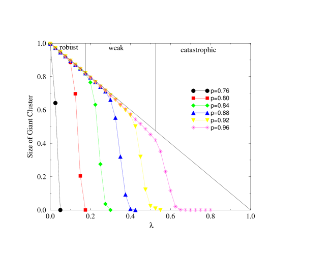
Figure 2: Turning off a scale free network. Three different phases in the behavior of the giant cluster size versus $\lambda$ (fraction of switched off nodes) are observed. These three phases are illustrated for $p=0.96$: the robust phase, the weak phase and the catastrophic phase (see the text). Other network parameters are as those of Fig. 1.

• Route II: By switching off a critical fraction of neurons for a fixed $p$. This is done by looking over all the elements of the network, and considering that the element activity is set to zero with probability $\lambda$ (which implies that on average $\lambda N$ elements are reset to zero). The result of this operation is shown in Fig. 2. Here, it is plotted for different $p$’s the relative size of the biggest (giant) cluster of connected active nodes in the network versus $\lambda$. Note that this procedure does not take into account the existence of connectivity classes, but all nodes are equally treated. The procedure is thus equivalent to simulations of random failure in percolation studies (Callaway et al., 2000). The strategy in which highly connected functional units are first put to zero is more aggressive and leads to quite different results.

  Each curve presents three different zones depending on $\lambda$:

  - the robust phase: For small $\lambda$, the network is stable and only those states put to zero have no activity. There is a linear dependence on the giant cluster size with $\lambda$. In this stage, the switched off nodes do not have the capacity to transmit its actual state to its active neighbors. • - the weak phase: For an intermediate $\lambda$, the nodes with null activity can influence its neighborhood and switch off some of them. The linearity between the size of the giant cluster and $\lambda$ shows a higher absolute value of the slope than in the robust zone. • - the catastrophic phase: When a critical $\lambda_{c}$ is reached, the system undergoes a crisis. The sudden drop in this zone means that a small increase of the non active nodes leads the system to a catastrophe; that is, the null activity is propagated through all the network and it becomes completely down.

It is worth noticing that when the system is outside the bistability region for $p>1$, the catastrophic phase does not take place. Instead, the turned off nodes do not spread its dynamical state and the neighboring nodes do not die out. This is because the dynamics of an isolated node is self-sustained when $p>1$. Consequently, we observe that the network breaks down in many small clusters and the transition resembles that of percolation in scale free nets (Callaway et al., 2000; Vazquez, & Moreno, 2003).

3.2 Switching on the network

Two equivalent strategies can be followed for the case of turning on the network (Fig. 3): (I) For a fixed $p$, we can increase the maximum value $\epsilon$ of the noisy signal, which is randomly distributed in the interval $(0,\epsilon)$ over the whole system. When $\epsilon$ attains a critical value $\epsilon_{c}$, the noisy configuration can leave the basin of attraction of $x_{\theta}$, which seems to have the form in phase space of a “hollow cane” (canuto) around it, and then the network rapidly evolves toward the turned on state; (II) If this operation is executed by letting $\epsilon$ to be fixed and by increasing the coupling parameter $p$, the final result of switching on the network is reached when $p$ takes the value for which $\epsilon=\epsilon_{c}$. The final result is identical in both cases.

Let us remark that the strategy equivalent to the former Route II is not possible in this case. It is a consequence of the fact that a switched off neuron can not be excited by its neighbors and it will maintain indefinitely the same dynamical state ($x_{i}=0$).

4 Conclusions

One of the most challenging scientific problems today is to understand how the millions of neurons of our brain give rise to the emergent property of thinking. Different aspects of neurocomputation take contact on this problem: how brain stores information and how brain processes it to take decisions or to create new information. These are characteristics more or less accepted and observed in all the brains.

Other universal properties of this system are more evident. One of them is the existence of a regular daily behavior: the awake and the sleep. The internal circadian rhythm is closely synchronized with the cycle of sun light. Roughly speaking and depending on the particular species, the brain is awake during the day and it is slept during the night, or vice versa. Hence, this evident bistability does not depend on the precise architecture of a special brain.

In this work, we have studied a general network with local logistic dynamics that presents global bistability between an active synchronized state and another synchronized state with no activity. This property is topology and size independent. This is a direct consequence of the local mean-field multiplicative coupling among the first-neighbors (the Alesves coupling). Different routes to transit from one state to the other have been explored for the important case of a scale free network. If a formal relationship is established between the switched on and switched off states of that network, and the awake and sleep states of a brain, respectively, one would be tempted to assert that this model is a good qualitative representation for explaining that specific bistable behavior. Other analogies could be suggested in reference to the usual functioning and the failures of a power line, or also the brain bistability in pattern recognition is another intriguing neural phenomenon. Furthermore, we are convinced that this model, regardless of its simplicity, can bring new qualitative insights on how the brain works.

Figures

Figure 1: Stable states $(x_{\theta},x_{+})$ of the network for $0<p<1$. Let us observe the two zones of bistability: $p_{0}<p<p_{c}$ and $p_{c}<p<p_{f}$. The main figure correspond to a scale free network made up of $N=10^{4}$ elements: $p_{0}=0.75$, $p_{c}=0.87\pm 0.01$ and $p_{f}=1$. The inset shows the same graph but in an all-to-all network of the same size: $p_{0}=0.75$, $p_{c}=p_{f}=1$. Initial conditions for the $x_{i}$’s were drawn from a uniform probability distribution in the interval $(0,1)$.

Figure 3: Turning on a scale free network. For a fixed $p$, a noisy signal randomly distributed in the interval $(0,\epsilon)$ is assigned to every node. When $\epsilon$ reaches the critical level $\epsilon_{c}$ the network becomes switched on. Other network parameters are as those of Fig. 1.

References

-
[1]
Barabási, A.-L., & Albert, R. (1999).
“Emergence of scaling in random networks,” Science 286, 509-512;
Barabási, A.-L., Albert, R., & Jeong, H. (1999). “Mean-field theory for scale-free random networks,” Physica A 272, 173-187. - [2] Bar-Yam, Y. (1997). Dynamics of Complex Systems,Westview Press.
- [3] Boccaletti, S., Kurths, J., Osipov, G., Valladares, D.L., & Zhou, C.S. (2002). “The synchronization of chaotic systems,” Phys. Rep. 366, 1-101.
- [4] Borgers, C., & Kopell, N. (2003). “Synchronization in networks of excitatory and inhibitory neurons with sparse, random connectivity,” Neural Comput. 15, 509-538.
- [5] Bornholdt, S., & Schuster, H.G. eds. (2002). Handbook of Graphs and Networks: From the Genome to the Internet, Wiley-VCH, Berlin.
- [6] Buzsàki, G., Geisler, C., Henze, D.A., & Wang, X.-J. (2004). “Interneuron diversity series: circuit complexity and axon wiring economy of cortical interneurons,” Trends in Neurosciences 27, 186-193.
- [7] Callaway, D.S., Newman, M.E.J., Strogatz, S.H., & Watts, D.J. (2000). “Network robustness and fragility: Percolation on random graphs,” Phys. Rev. Lett. 85, 5468-5471.
- [8] Dorogovtsev, S.N., & Mendes, J.F.F. (2003). Evolution of Networks. From Biological Nets to the Internet and the WWW, Oxford University Press, Oxford.
- [9] Eguiluz, V.M., Chialvo, D.R., Cecchi, G., Baliki, M., & Apkarian, A.V. (2003). “Scale-free brain functional networks,” preprint in cond-mat/0309092.
- [10] Hansel, D., & Mato, G. (2003). “Asynchronous states and the emergence of synchrony in large networks of interacting excitatory and inhibitory neurons,” Neural Comput. 15, 1-56.
- [11] Jalan, S., & Amritkar, R.E. (2003). “Self-organized and driven phase synchronization in coupled maps,” Phys. Rev. Lett. 90, 014101(4) (2003).
- [12] López-Ruiz, R., & Fournier-Prunaret, D. (2004). “Complex behavior in a discrete logistic model for the symbiotic interaction of two species,” Mathematical Biosciences and Engineering 1 (2), to appear.
- [13] López-Ruiz, R., & Fournier-Prunaret, D. (2003). “Complex patterns on the plane: different types of basin fractalization in a two-dimensional mapping,” Int. J. of Bifurcation and Chaos 13, 287-310.
- [14] May, R.M. (1976). “Simple mathematical models with very complicated dynamics,” Nature 261 459-467.
- [15] Moreno, Y., Pastor-Satorras, R., & Vespignani, A. (2002). “Epidemic outbreaks in complex heterogeneous networks,” Eur. Phys. J. B 26, 521-529.
- [16] Pastor-Satorras, R., & Vespignani, A. (2004). Evolution and Structure of the Internet, Cambridge University Press, Cambridge.
- [17] Sima, J., & Orponen, P. (2003). “General-purpose computation with neural networks: A survey of complexity theoretic results,” Neural Comput. 15, 2727-2778.
- [18] Strogatz, S.H. (2001). “Exploring complex networks,” Nature (London) 410, 268-276.
- [19] Vázquez, A., & Moreno, Y. (2003). “Resilience to damage of graphs with degree correlations,” Phys. Rev. E 67, 015101(R).
- [20] Winfree, A.T. (1986). The timing of biological clocks, Scientific American Library, W.H. Freeman Co.