Stabilization of a light bullet in a layered Kerr medium with sign-changing nonlinearity

Abstract

Using the numerical solution of the nonlinear Schrödinger equation and a variational method it is shown that (3+1)-dimensional spatiotemporal optical solitons, known as light bullets, can be stabilized in a layered Kerr medium with sign-changing nonlinearity along the propagation direction.

I Introduction

After the prediction of self-trapping st of an optical beam in a nonlinear medium resulting in an optical soliton 1 , there have been many theoretical and experimental studies to stabilize such a soliton under different conditions of nonlinearity. A bright soliton in (1+1) dimension (D) in Kerr medium is unconditionally stable for positive or self-focusing (SF) nonlinearity in the nonlinear Schrödinger equation (NLS) 1 . However, in (2+1)D in homogeneous bulk Kerr medium one cannot have a stable soliton-like axisymmetric cylindrical beam 2 ; 3 ; 3a . Also, in (3+1)D in such a medium one cannot have a stable optical wave packet that remain confined in all directions. Such a confined wave packet in (3+1)D is often called a light bullet and represents the extension of a self-trapped optical beam into the temporal domain 1 . If the nonlinearity is negative or self-defocusing (SDF), any initially created soliton spreads out in both (2+1)D and (3+1)D 1 . If the nonlinearity is positive or of SF type, any initially created soliton is unstable and eventually collapses 1 .

Recently, through a numerical simulation as well as a variational calculation based on the NLS it has been shown that the axisymmetric cylindrical beam in (2+1)D can be stabilized in a layered medium if a variable nonlinearity coefficient is used in different layers mal ; ber . A weak modulation of the nonlinearity coefficient along the propagation direction leads to a reasonable stabilization in (2+1)D ber . A much better stabilization results if the Kerr coefficient is a layered medium is allowed to vary between successive SDF and SF type nonlinearities, i.e., between positive and negative values mal . However, it has been shown that such a modulation of the nonlinearity coefficient in a Kerr medium should fail to achieve stabilization of a light bullet abdul or a general three-dimensional soliton new .

As the stabilization of a light bullet is of utmost interest, we revisit this problem and find, to great surprise, that a spatiotemporal light bullet can be stabilized in a layered Kerr medium with sign-alternating nonlinearity along the propagation direction.

Although, the present work is of interest from a theoretical point of view, it also has phenomenological or experimental consequences. Recently, it has been emphasized liu that large negative values of the Kerr coefficient can be created by using the cascading mechanism with a large phase-mismatch parameter. It has also been suggested xxx that a layered medium with alternating sign of nonlinearity can be created with the technique of mesoscopic self-organization. Hence a stabilized light bullet can be experimentally realized in the future.

To stabilize a soliton in a SF homogeneous bulk Kerr medium, the repulsive kinetic pressure due to the Laplacian operator in space and time in the NLS has to balance the attraction due to nonlinearity. For a light bullet of size $L$, kinetic pressure is proportional to $L^{-2}$ whereas attraction is proportional to $L^{-D}$ in $(D+1)$ D. The effective potential, which is a sum of these two terms, has a confining minimum only for $D=1$ leading to a stable soliton ueda . Using a variational method we find that a layered Kerr medium with sign-changing nonlinearity in (3+1)D can lead to an effective potential with a minimum which can stabilize the solitons.

In Sec. II we present a variational study of the problem and in Sec. III we present a complete numerical study. Finally, in Sec. IV we give the concluding remarks.

II Variational Calculation

For anomalous dispersion, the NLS can be written as 1

$$\biggr{[}i\frac{\partial}{\partial z}+\frac{1}{2}\nabla_{r}^{2}+\gamma(z)|{u({\bf r},z)}|^{2}\biggr{]}u({\bf r},z)=0,$$ (1)

where in (3+1)D the three dimensional vector ${\bf r}$ has space components $x$ and $y$ and time component $t$, and $z$ is the direction of propagation. The Laplacian operator $\nabla_{r}^{2}$ acts on the variables $x$, $y$, and $t$. In (2+1)D in Eq. (1) the vector ${\bf r}$ could have components $x$ and $y$ or $x$ and $t$, while $z$ continues as the direction of propagation. The nonlinearity coefficient $\gamma(z)$ in a layered Kerr medium is piecewise continuous and can have successive positive (SF) and negative (SDF) values $\gamma_{+}$ and $\gamma_{-}$ in layers of width $d$. The normalization condition is $\int d{\bf r}|u({\bf r},z)|^{2}=P$, where $P$ is the power of the optical beam st ; mal .

For a spherically symmetric soliton in (3+1)D, $u({\bf r},z)=U(r,z)$. Then the radial part of the NLS (1) becomes 1

$$\biggr{[}i\frac{\partial}{\partial z}+\frac{1}{2}\frac{\partial^{2}}{\partial r^{2}}+\frac{1}{r}\frac{\partial}{\partial r}+\gamma(z)\left|{U({r},z)}\right|^{2}\biggr{]}U({r},z)=0.$$ (2)

In the following we consider variational and numerical solutions of Eq. (2).

First we consider the variational approach with the following trial Gaussian wave function for the solution of Eq. (2) ueda ; abdul

$$U(r,z)=N(z)\exp\left[-\frac{r^{2}}{2R^{2}(z)}+\frac{i}{2}{b(z)}r^{2}+i\alpha(z)\right],$$ (3)

where $N(z)$, $R(z)$, $b(z)$, and $\alpha(z)$ are the soliton’s amplitude, width, chirp, and phase, respectively. In Eq. (3) in (3+1)D $N(z)={P^{1/2}}/{[\pi^{3/4}R^{3/2}(z)]}$. The trial function (3) satisfies (a) the normalization condition st ; mal as well as the boundary conditions (b) $U(r,z)\to$ constant as $r\to 0$ and (c) $|U(r,z)|$ decays exponentially as $r\to\infty$ mal .

The Lagrangian density for generating Eq. (2) is abdul

$${\cal L}(U)=\frac{i}{2}\left(\frac{\partial U}{\partial z}U^{*}-\frac{\partial U^{*}}{\partial z}U\right)-\frac{1}{2}\left|\frac{\partial U}{\partial r}\right|^{2}+\frac{\gamma|U|^{4}}{2}.$$ (4)

The trial function (3) is substituted in the Lagrangian density and the effective Lagrangian is calculated by integrating the Lagrangian density: $L_{\mbox{eff}}=\int{\cal L}(U)d\bf r.$ The Euler-Lagrange equations for $R(z)$, $b(z)$, and $\alpha(z)$ are then obtained from the effective Lagrangian in standard fashion mal ; abdul ; ueda . Eliminating $\alpha(z)$, the equations for $b(z)$ and $R(z)$ in (3+1)D can be written as

$$\frac{dR(z)}{dz} = R(z)b(z),$$ (5)

$$\frac{db(z)}{dz} = \frac{1}{R^{4}(z)}-b^{2}(z)-\frac{\gamma(z)P}{2\sqrt{2\pi^{3}}}\frac{1}{R^{5}(z)}.$$ (6)

From Eqs. (5) and (6) we get the following second-order differential equation for the evolution of the width

$$\frac{d^{2}R(z)}{dz^{2}}=\frac{1}{R^{3}(z)}-\frac{\gamma(z)P}{2\sqrt{2\pi^{3}}R^{4}(z)}.$$ (7)

Here we re-visit the stability condition of light bullets of Eq. (7) for $\gamma(z)=\gamma_{0}+\gamma_{1}(z)$, where $\gamma_{0}=g_{0}$ is a positive constant of SF type and $\gamma_{1}(z)$ is a rapidly varying part with zero mean value. We take $\gamma_{1}(z)=g_{1}\sin(\omega z)$, as this is a form that we can integrate easily. We break $R(z)$ into a slowly varying part $A(z)$ and a rapidly varying part $B(z)$ by $R(z)=A(z)+B(z)$. Substituting this into Eq. (7) and retaining terms of the order of $\omega^{-2}$ in $B(z)$ we obtain the following equations of motion for $B(z)$ and $A(z)$:

$$\frac{d^{2}B(z)}{dz^{2}} = -\frac{g_{1}P\sin(\omega z)}{2\sqrt{2\pi^{3}}A^{4}(z)},$$ (8)

$$\frac{d^{2}A(z)}{dz^{2}}=\frac{1}{A^{3}(z)}-\frac{g_{0}P}{2\sqrt{2\pi^{3}}A^{4}(z)}+\frac{2g_{1}P\langle{B(z)\sin(\omega z)}\rangle}{\sqrt{2\pi^{3}}A^{5}(z)},$$ (9)

where $\langle\quad\rangle$ denotes time average over rapid oscillation. Using the solution $B(z)=g_{1}P\sin(\omega z)/[2\sqrt{2\pi^{3}}\omega^{2}A^{4}(z)]$, the equation of motion for $A(z)$ becomes

$$\frac{d^{2}A(z)}{dz^{2}} = \frac{1}{A^{3}}-\frac{g_{0}P}{2\sqrt{2\pi^{3}}A^{4}}+\frac{g_{1}^{2}P^{2}}{4\pi^{3}\omega^{2}A^{9}},$$ (10)

$$= -\frac{\partial}{\partial A}\left[\frac{1}{2A^{2}}-\frac{g_{0}P}{6\sqrt{2\pi^{3}}A^{3}}+\frac{g_{1}^{2}P^{2}}{32\pi^{3}\omega^{2}A^{8}}\right].$$ (11)

The quantity in the square bracket in Eq. (11) is the effective potential $U(A)$ of the equation of motion

$$U(A)=\frac{1}{2A^{2}}-\frac{g_{0}P}{6\sqrt{2\pi^{3}}A^{3}}+\frac{g_{1}^{2}P^{2}}{32\pi^{3}\omega^{2}A^{8}}.$$ (12)

Stabilization is possible when there is a minimum in this effective potential ueda . Unfortunately, this condition does not lead to a simple analytical solution. However, straightforward numerical study reveals that this effective potential has a minimum for a positive $g_{0}P$ corresponding to attraction (SF nonlinearity) with $g_{0}P$ above a critical value. For a numerical calculation the quantity $gP$ is taken to be of the form $gP=g_{0}P+g_{1}P\sin(\omega z)\equiv g_{0}P[1+4\sin(10\pi z)]$, so that $g_{1}=4g_{0}$ and $\omega=10\pi$. The numerical values for $g_{1}$ and $\omega$ are taken as examples, otherwise they do not have great consequence on the result so long as $\omega$ is large corresponding to rapid oscillation. In Fig. 1 (a) we plot the effective potential $U(A)$ vs. $A$ for $g_{0}P=30,100,200$, and 500 for $\omega=10\pi$. For $g_{0}P=30$ there is no minimum in $U(A)$, whereas a minimum has appeared for $g_{0}P=100$ which becomes deeper for $g_{0}P=200$ and 500. A careful examination reveals that the threshold for the minimum in the present case is given by $g_{0}P\approx 40$. Hence in the present case stabilization is not possible for $g_{0}P=30$, and it is possible for $g_{0}P>40$. There is no upper limit for $g_{0}P$ and stabilization seems possible for an arbitrarily large $g_{0}P$. As $g_{0}P$ increases the depth of the effective potential in Fig. 1 (a) increases and consequently, it is easier to stabilize a soliton. As the first and the third terms on the right hand side (rhs) of Eq. (10) are positive, no stabilization is possible for a negative $g_{0}P$ corresponding to repulsion (SDF).

In order to see the effect of the frequency $\omega$ on stabilization, we plot in Fig. 1 (b) the same effective potentials of Fig. 1 (a) for $\omega=30\pi$. With the increase of $\omega$ the effective potentials have become deeper and hence the stabilization easier. For $g_{0}P=30$ we have a minimum in Fig. 1 (b) whereas there is no minimum in Fig. 1 (a). With the increase of $\omega$ the threshold value of $g_{0}P$ for obtaining a minimum has reduced.

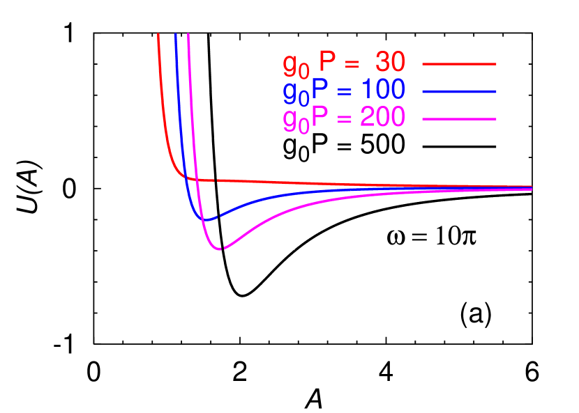
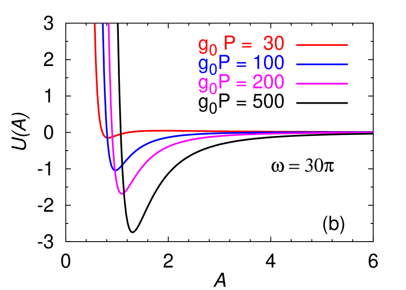
Figure 1: The effective potential $U(A)$ of Eq. (12) vs. $A$ in arbitrary units for $g_{0}P=30,100,200,500$ (from shallower to deeper minimum), for (a) $\omega=10\pi$ and (b) $\omega=30\pi$.

The sinusoidal variations of Kerr nonlinearity as considered above for variational study only simplifies the algebra and is by no means necessary for stabilization of solitons. In the following numerical study we establish that a rapid oscillation of the nonlinearity coefficient between positive and negative values also stabilizes the soliton in (3+1)D.

III numerical calculation

We solve Eq. (2) numerically using the split-step time-iteration method employing the Crank-Nicholson discretization scheme 11 . The time iteration is started with the known solution of some auxiliary equation with zero nonlinearity. The auxiliary equations with known Gaussian solution are obtained by adding a harmonic oscillator potential $r^{2}$ to Eq. (2). Then in the course of time iteration the power $P$ and a positive constant SF Kerr nonlinearity $\gamma(z)=g_{0}=1$ is switched on slowly and the harmonic trap is also switched off slowly. If the nonlinearity is increased rapidly the system collapses. The tendency to collapse or expand must be avoided to obtain a stabilized soliton.

After switching off the harmonic trap in Eq. (2) and after slowly introducing the final power $P$ and the constant nonlinearity $\gamma(z)=g_{0}=1$, an oscillating Kerr nonlinearity $\gamma_{1}(z)$ oscillating between $\pm g_{1}$ $(|g_{1}|>1)$ like a step function as $z$ changes by $d$ is introduced on top of the constant nonlinearity. The overall Kerr nonlinearity now has successive positive and negative values $\gamma_{+}=1+g_{1}$ and $\gamma_{-}=1-g_{1}$ of equidistant layers of width $d$ in $z$ direction. A stabilization of the final solution could be obtained for a suitably chosen $\gamma_{\pm}$ and a small $d$. If the SF power after switching off the harmonic trap is large compared to the spatiotemporal size of the beam the system becomes highly attractive in the final stage and it eventually collapses. If the final power after switching off the harmonic trap is small for its size the system becomes weakly attractive in the final stage and it expands. The final nonlinearity has to have an appropriate intermediate value, decided by trial, for final stabilization. The stabilization could be obtained for a large range of values of $\gamma_{\pm}$ and $d$. After some experimentation with Eq. (2) we opted for the choice $\gamma_{+}=5$, $\gamma_{-}=-3$, and $d=0.1$ in all our calculations.

In the present scheme of stabilization the nonlinearity rapidly fluctuates between appropriate positive (SF) and negative (SDF) values in the propagation direction. For positive nonlinearity, the system tends to collapse, whereas in the SDF regime it tends to expand to infinity. If the nonlinerities are appropriate, the collapse in the first interval is exactly compensated for by the expansion in the next interval and a stabilization of the system is obtained. Obviously, the system will be more stable when the intervals are small so that the fluctuation of the system around a stable mean position is small. Consequently, the system remains virtually static and the very small oscillations arising from collapse and expansion remain unperceptable.

Although, for the sake of convenience we applied a harmonic trap in the beginning of our simulation, which is removed later with the increase of nonlinearity, this restriction is by no means necessary for stabilizing a soliton. Saito et al. ueda used a qualitatively similar, but quantitatively different, procedure for stabilization in the context of Bose-Einstein condensation in two dimensions. The procedure of Saito et al. could also be applied sucessfully in the present context.

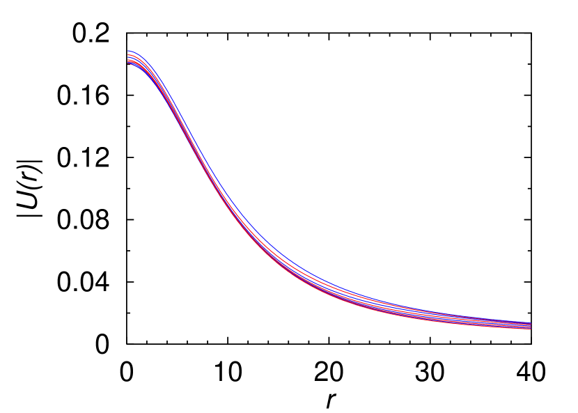
Figure 2: Wave function $|U(r)|$ of Eq. (2) of stabilized light bullet of power $P=682.6$ and $\langle\gamma(z)\rangle=g_{0}=1$ and $\gamma_{1}(z)$ oscillating between $\gamma_{+}=5$ and $\gamma_{-}=-3$ in successive layers of width $d=0.1$ in the $z$ direction. The wave functions are shown at positions $z=0,50,100,150,200,250,300,350$ and 400.

Now we turn to a numerical investigation of Eq. (2). The results are shown in Fig. 2 for the (3+1) dimensional soliton, where we plot the radial part of the wave function for different $z$ for a power $P=682.6$. A finetuning of the power was needed for the stabilization reported in Fig. 2.

In Fig. 2 the narrow spread of the wave function over the large interval of $z$ shows the quality of stabilization. The results at intermediate $z$ lie in the region covered by the plots. The plot of the full wave function at different $z$ on the same graph clearly shows the degree of stabilization achieved. The stabilization seems to be perfect and can easily be continued for longer intervals of $z$ by increasing the power. In Ref. mal layers of width $d=0.001$ was employed for stabilization in (2+1)D. The present stabilization is obtained with a much larger width $d=0.1$, which make the present proposal more attractive from a phenomenological point of view. The stabilization can only be obtained for beams with power larger than a critical value. Numerically, we found it was easier to obtain stabilization of beams with power much larger than the critical value. In (3+1)D good stabilization could be obtained for much larger power: the power employed in Fig. 2 was 682.6, whereas the critical variational power for stabilization obtained in Fig. 1 is about 40.

Using a variational procedure alone, not quite identical with the present approach, in the context of Bose-Einstein condensation Abdullaev et al. abdul also had found that a stabilization of a soliton could be possible in (3+1)D via a temporal modulation of the nonlinearity. However, they confirmed after further analytical and numerical study that such a stabilization does not take place in (3+1)D. Saito et al. ueda and Towers et al. mal , on the other hand, are silent about the possibility of the stabilization of a soliton in (3+1)D. We point out one possible reason for the negative result obtained by Abdullaev et al. abdul in (3+1)D. The nonlinearity parameter $\lambda_{0}N=\sqrt{2}\pi^{3/2}\Lambda$ with $\Lambda=1$ used in Ref. abdul for stabilizing a soliton in (3+1)D is much too small (smaller than the threshold discussed in Sec. II). Comparing Eq. (2) of abdul with our Eq. (2) we find that the above value of nonlinearity corresponds in our notation to $g_{0}P=\lambda_{0}N/2=\pi^{3/2}/\sqrt{2}\approx 3.9$, whereas the present variational threshold for obtaining a stabilized soliton is $g_{0}P\approx 40$. The very small nonlinearity used in Ref. abdul is most possibly the reason for the negative result obtained there. More recently, Montesinos et al. new have also confirmed the conclusion of Ref. abdul that no stable three-dimensional soliton could be obtained by a variation of Kerr nonlinearity. However, they did not give details of their study, which led to this conclusion, for a comparison.

IV Conclusion

In conclusion, after a variational and numerical study of the NLS we find that it is possible to stabilize a spatiotemporal light bullet in (3+1)D by employing a layered Kerr medium with a sign-changing nonlinearity along the propagation direction. From a variational calculation we show that a oscillating Kerr nonlinearity produces a minimum in the effective potential, thus producing a potential well in which the soliton can be trapped. The present stabilized soliton is a slowly collapsing Townes soliton [1] with large power. The oscillating Kerr nonlinearity stops the collapse and enhances the lifetime of the soliton greatly. This is of interest to investigate if such light bullets could be created experimentally.

Apart from optics, such stable three-dimensional solitons can be realized experimentally in Bose-Einstein condensates (BEC), where a Feshbach resonance could be used to generate an oscillating nonlinearity or an oscillating effective interatomic interaction via the modulation of an external background magnetic field abdul ; ueda . The stabilization of such BEC solitons in two abdul ; ueda ; new and three unp dimensions is already under investigation.

- (1) R. Y. Chiao, E. Garmire, and C. H. Townes, Phys. Rev. Lett. 13, 479 (1964).
- (2) A. Hasegawa and F. Tappert, Appl. Phys. Lett. 23, 171 (1973), 23, 142 (1973); V. E. Zakharov and A. B. Shabat Sov. Phys. JETP 34, 62 (1972), 37, 823 (1973).
- (3) Y. S. Kivshar and G. P. Agrawal, Optical Solitons - From Fibers to Photonic Crystals, (Academic Press, San Diego, 2003).
- (4) V. I. Kruglov and R. A. Vlasov, Phys. Lett. 111A, 401 (1985).
- (5) W. J. Firth and D. V. Skryabin, Phys. Rev. Lett. 79, 2450 (1997); D. V. Skryabin and W. J. Firth, Phys. Rev. E 58, 3916 (1998); J. Atai, Y. Chen, and J. M. Soto-Crespo, Phys. Rev. A 49, R3170 (1994).
- (6) V. V. Afanasjev, Phys. Rev. E 52, 3153 (1995).
- (7) I. Towers and B. A. Malomed, J. Opt. Soc. Am. B 19, 537 (2002).
- (8) L. Bergé, V. K. Mezentsev, J. J. Rasmussen, P. L. Christiansen, and Yu. B. Gaididei, Opt. Lett. 25, 1037 (2000).
- (9) F. K. Abdullaev, J. G. Caputo, R. A. Kraenkel, and B. A. Malomed, Phys. Rev. A 67, 013605 (2003).
- (10) G. D. Montesinos, V. M. Perez-Garcia, and P. J. Torres, Physica D 191, 193 (2004).
- (11) L. J. Qian, X. Liu, and F. W. Wise, Opt. Lett. 24, 166 (1999); X. Liu, L. J. Qian, and F. W. Wise, ibid. 24, 1777 (1999).
- (12) L. Brzozowski and E. H. Sargent, IEEE J. Quantum Electron. 36, 550 (2000).
- (13) H. Saito and M. Ueda, Phys. Rev. Lett. 90, 040403 (2003).
- (14) S. K. Adhikari and P. Muruganandam, J. Phys. B 35, 2831 (2002); 36, 409 (2003); P. Muruganandam and S. K. Adhikari, ibid. 36, 2501 (2003).
- (15) S. K. Adhikari, Phys. Rev. A 69 063613 (2004).