Euler-Poincaré formulation and elliptic instability for $n^{th}-$gradient fluids

Abstract

The energy of an $n^{th}-$gradient fluid depends on its Eulerian velocity gradients of order $n$. A variational principle is introduced for the dynamics of $n^{th}-$gradient fluids and their properties are reviewed in the context of Noether’s theorem. The stability properties of Craik-Criminale solutions for first and second gradient fluids are examined.

1 Introduction

Classical continuum theories lack any length scales and as such provide leading order approximations for a number of problems that contain microstructures. Microstructures typically introduce characteristic length scales that may induce gradient dependences of various kinds. Several continuum theories have been developed to deal with microstructures and their attendant phenomena. These include micropolar, micromorphic, strain-gradient, non-local, etc. See Eringen [1] and Nowacki [2] for catalogs of such phenomenological theories. Physical theories for complex fluids such as liquid crystals have also been introduced, based on symmetry breaking phase transitions that yield statistically-defined order parameters as additional thermodynamic variables. See de Gennes and Prost [3] for discussions of the fundamental principles of order parameter physics for liquid crystals. See Holm [4] for a variational description of order parameter theories of complex fluids. Often these phenomenological theories are combined with geometrical discussions based on the theory of Cosserat and Cosserat [5].

The mathematical theory of continuum mechanics for complex, or composite materials produced a number of interesting phenomenological models in the 1960’s. Among these are the models of differential type introduced by Rivlin and Ericksen [6] and the multipolar models of Green and Rivlin [7, 8]. The history of how these models were tested in comparison with experiments and refined by ab initio assumptions of thermodynamics is recounted, for example, in Dunn and Fosdick [9], Eringen [1] and Fosdick and Rajagopal [10].

Recently, Bellout et al[11] considered a fusion of the models due to Rivlin and Ericksen [6] and those of Green and Rivlin [7, 8]. The resulting theory introduced higher order spatial velocity gradients into the energy that regularized the model solutions and endowed the model with promising stability characteristics.

The present work specializes to a subclass of the Rivlin-Ericksen-Green multipolar fluids treated in Bellout et al[11] that has energy density given by

$${{\textstyle\frac{1}{2}}}D|{\mathbf{u}}|^{2}+DW(\mathbf{e},\nabla\mathbf{e},\nabla\nabla\mathbf{e},\dots,D,\nabla{D},\nabla\nabla{D},\dots),$$ (1)

where $D$ is the mass density and $\mathbf{e}={{\textstyle\frac{1}{2}}}(\nabla{\mathbf{u}}+\nabla{\mathbf{u}}^{T})$ is the strain rate tensor. Materials whose energy density takes this form are called gradient fluids of degree $n$, where $n$ is the order of the velocity gradients appearing in (1). The case $n=0$ is the Euler fluid (no velocity gradient dependence), while the case $n=1$ coincides with the $2^{nd}$ grade fluid [9], whose energy depends on the velocity gradient through the strain-rate, $\mathbf{e}$.

Our aim here is to investigate the implications of adopting a subclass of these $n^{th}-$gradient models for the well-known elliptic instability, which governs the rapid, violent transition from two-dimensional to three-dimensional motion at the onset of turbulence in Newtonian fluids [12, 13, 14, 15, 16]. We shall not assess the implications for experimental measurements of this investigation, as we feel that such an assessment may still be premature. Instead, we continue the investigation begun by Bellout et al[11] in studying the role of $n^{th}-$gradient constitutive relations on fluid instability. We begin by casting the $n^{th}-$gradient theory of nonlinear elasticity into the Euler-Poincaré variational framework [17]. The Euler-Poincaré framework allows us to take advantage of several parallels between $n^{th}-$gradient fluids and recently developed Lagrangian-averaged Navier-Stokes-alpha, or LANS$-\alpha$, turbulence closure models of Foias et al[18]. Since Rivlin [19], remarkable parallels have been drawn between nonlinear elasticity and turbulence closure models. In our case, the Euler-Poincaré framework leads to energy balance laws, a proper definition of momentum density, circulation theorems and to the Craik-Criminale (CC) class of exact solutions for the $n^{th}-$gradient materials.

The CC solutions [20] form the basis for analyzing elliptic instability, in which two-dimensional flows with closed streamlines are subject to three-dimensional instabilities. Our aim in this paper is to determine the effects of $n^{th}-$gradient viscoelasticity on the parametric resonance mechanism responsible for elliptic instability and on its growth rates. We follow the earlier treatment of elliptic instability for Newtonian fluids as reviewd, e.g., by Kerswell [16], and we are guided by the results of Fabijonas and Holm [21, 22] based on the CC solutions for the LANS$-\alpha$ and similar closure models for turbulence. Thus, we consider plane wave disturbances of elliptical flows whose wave amplitude and wave vector are time-dependent. This approach leads to a Floquet problem for the wave amplitude of the disturbance. Remarkably, we discover that these viscoelastic effects may be either stabilizing, or destabilizing, in the sense that they alter the shape and size of the instability domain while simultaneously increasing or decreasing the associated Lyapunov growth rates, depending on the parameter values. We hope that experimentalists may be guided by these results in testing whether $n^{th}-$gradient models may be appropriate for the description of viscoelastic materials undergoing elliptic instability.

The equations of motion for gradient fluids are obtained from the Eulerian form of Hamilton’s principle introduced in Holm, Marsden and Ratiu [17] called the Euler-Poincaré theory for continua with advected quantities. In vector notation, this is

$$\frac{\partial}{\partial t}{\mathbf{m}}+{\mathbf{u}}\cdot\nabla{\mathbf{m}}+(\nabla{\mathbf{u}})^{T}\cdot{\mathbf{m}}+{\mathbf{m}}{\rm\,div\,}{\mathbf{u}}-\nabla\frac{\delta{L}}{\delta D}=0\,,\,\,\hbox{where}\,\,{\mathbf{m}}\equiv\frac{\delta{L}}{\delta{\mathbf{u}}}\,.$$ (2)

For the class of Lagrangians we shall consider, for $0^{th}$, $1^{st}$ and $2^{nd}$ gradient fluids, one has

$${L}=\int d^{3}x\Big{\{}{{\textstyle\frac{1}{2}}}D|{\mathbf{u}}|^{2}+D{\mathbf{u}}\cdot{\mathbf{R}}({\mathbf{x}})-p(D-1)+DW(\mathbf{e},\nabla\mathbf{e})\Big{\}}\,.$$ (3)

The term in ${\mathbf{R}}$ in this Lagrangian boosts the gradient fluid flow into a frame rotating with angular frequency $2{\mathbf{\Omega}}={\rm curl}\,{\mathbf{R}}$, while the term in $p$ imposes the constraint $D=1$. Hence $\nabla\cdot{\mathbf{u}}=0$, as implied by substituting $D=1$ into the continuity equation,

$$\partial_{t}D+\nabla\cdot(D{\mathbf{u}})=0\,.$$ (4)

Many mathematical regularity properties are available for the class of gradient fluids, especially for the case that the Lagrangian $L$ in (3) provides a norm (when evaluated on the constraint surface, $D=1$). However, these regularity properties for gradient fluids will be discussed elsewhere, following Foias et al[23].

The objective of the current paper is to investigate the stability properties of CC solutions of the gradient fluid equations. For CC solutions in an unbounded domain, the fluid velocity is linear in the spatial coordinate and the pressure is quadratic. The CC solutions may be regarded as the first term in a Taylor expansion in space, around a stagnation point of the gradient fluid flow in a moving frame. We shall use the theory of elliptic instability to investigate the exact nonlinear growth rates when CC solutions interact with a wave packet whose phase is frozen into the CC flow for gradient fluids of degree $n=1,2$. (The Euler case $n=0$ was studied in the original work of Craik and Criminale [20]. See also Craik [24], Miyazaki [25] and Kerswell [16] for subsequent developments. See also Lagnado and Simmen [26] and Goddard and Alam [27] for similar analyses for an upper-convected Maxwell fluid and granular media, respectively.)

Outline.

Section 2 summarizes the properties of ideal gradient fluids that follow directly from their Euler-Poincaré formulation. These properties include energy conservation, momentum balance and Kelvin circulation preservation, all of which follow from Noether’s theorem. We then specialize to gradient fluids of degree $n=1,2$. Section 3 introduces the CC solutions for $1^{st}$ and $2^{nd}$ gradient fluids. Section 4 discusses their stability properties for both inviscid and viscous CC solutions. Here we introduce viscosity as in the theory of $2^{nd}$ grade fluids, to which the gradient fluids reduce when $n=1$. Section 5 summarizes our conclusions.

2 EP formulation of gradient fluids

Hamilton’s principle for first and second gradient fluids.

The mathematical basis common to all ideal fluid motions is Hamilton’s principle

$$\delta\int{L}~{}dt=0,$$ (5)

where ${L}$ is the Lagrangian for the system. We work in the Eulerian representation of fluids, where the Euler-Lagrange equation is replaced by the Euler-Poincaré equation. See Ref. [17] for a detailed discussion of Euler-Poincaré theory.

This paper focuses on the incompressible motion of first and second gradient fluids in a rotating frame. Thus, the class of Lagrangians we shall consider has the form [17]

$${L}=\int\mathcal{L}({\mathbf{u}},\nabla{\mathbf{u}},\nabla\nabla{\mathbf{u}},\dots,D,\nabla{D},\nabla\nabla{D},\dots;{\mathbf{R}}({\mathbf{x}}))\,d^{3}x\,,$$ (6)

where ${\mathbf{R}}({\mathbf{x}})$ is the vector potential for the Coriolis parameter, i.e., ${\rm curl}\,{\mathbf{R}}=2{\mathbf{\Omega}}$. Specifically, we shall take,

$${L}=\int d^{3}x\Big{\{}{{\textstyle\frac{1}{2}}}D|{\mathbf{u}}|^{2}+D{\mathbf{u}}\cdot{\mathbf{R}}({\mathbf{x}})-p(D-1)+DW(\mathbf{e},\nabla\mathbf{e})\Big{\}}\,.$$ (7)

Here $p$ is pressure (a Lagrange multiplier), $D$ is mass density, and ${\mathbf{u}}$ is fluid velocity. Through the function $W(\mathbf{e},\nabla\mathbf{e})$, the first and second gradient fluids depend on $\mathbf{e}$, the symmetric strain-rate tensor,

$$e_{ij}={{\textstyle\frac{1}{2}}}(u_{i,j}+u_{j,i})=\frac{1}{2}\left(\frac{\partial u_{i}}{\partial x^{j}}+\frac{\partial u_{j}}{\partial x^{i}}\right)\,.$$ (8)

That is, first and second gradient fluids allow energy to depend upon strain-rate $\mathbf{e}$ and gradient of strain-rate $\nabla\mathbf{e}$, respectively, [1, 9, 10]. The higher gradient fluids will allow energies that depend upon higher-order gradients of strain-rate. We introduced the dependence on $\mathbf{e}$, $\nabla\mathbf{e}$, etc., instead of $\nabla\mathbf{u}$, $\nabla\nabla\mathbf{u}$, etc., in equation (7), so that the Lagrangian $L$ will be invariant under rotations. Consequently, the resulting Euler-Poincaré equations will admit an angular momentum balance relation and will satisfy the requirements of material frame indifference.

Variational derivatives and natural boundary conditions.

The variational derivatives of the Lagrangian (7) for first and second gradient fluids are given by

$$\delta{L}=\int d^{3}x\Big{\{}D({\mathbf{u}}+{\mathbf{R}})\cdot\delta{\mathbf{u}}+\left({{\textstyle\frac{1}{2}}}|{\mathbf{u}}|^{2}+{\mathbf{u}}\cdot{\mathbf{R}}+W-p\right)\delta D-(D-1)\delta p+\boldsymbol{\sigma:\,}\delta\mathbf{e}\Big{\}},$$ (9)

where $\boldsymbol{\sigma:\,}\delta\mathbf{e}={\rm\,tr}(\boldsymbol{\sigma^{T}\cdot\,}\delta\mathbf{e})=\sigma^{ij}\delta{e}_{ij}$, and we sum over repeated indices. The quantity $\boldsymbol{\sigma}$ is the stress tensor, whose definition assures that it is symmetric, $\boldsymbol{\sigma^{T}}=\boldsymbol{\sigma}$,

$$\sigma^{ij}\equiv\frac{\delta{L}}{\delta e_{ij}}=D\,\frac{\partial W}{\partial e_{ij}}-\nabla\cdot D\,\frac{\partial W}{\partial\nabla e_{ij}}\,.$$ (10)

The added natural boundary condition for second gradient fluids,

$${\mathbf{\hat{n}}}\cdot\frac{\partial W}{\partial\nabla e_{ij}}\delta e_{ij}=0\,,$$ (11)

arises from an integration by parts. Another application of integration by parts and use of the symmetry of $e_{ij}$ gives

$$\delta{L}=\int d^{3}x\Big{\{}D({\mathbf{u}}+{\mathbf{R}}-\nabla\cdot{\boldsymbol{\sigma}})\cdot\delta{\mathbf{u}}+({{\textstyle\frac{1}{2}}}|{\mathbf{u}}|^{2}+{\mathbf{u}}\cdot{\mathbf{R}}+W-p)\delta D-(D-1)\delta p\Big{\}},$$ (12)

where $(\nabla\cdot{\boldsymbol{\sigma}})^{i}=\partial\sigma^{ij}/\partial x^{j}$. Another natural boundary condition has been introduced and applied,

$${\mathbf{\hat{n}}}\cdot{\boldsymbol{\sigma}}\cdot\delta{\mathbf{u}}=0\,,\quad\hbox{at the boundary.}$$ (13)

This condition may be satisfied when the fluid velocity has no normal component at the boundary, by requiring that the normal stress have no tangential component,

$$({\mathbf{\hat{n}}}\cdot{\boldsymbol{\sigma}})\times{\mathbf{\hat{n}}}=0\,,\quad\hbox{at the boundary.}$$ (14)

The Euler-Poincaré motion equation.

The Euler-Poincaré motion equation is [17]

$$\frac{\partial}{\partial t}{\mathbf{m}}+{\mathbf{u}}\cdot\nabla{\mathbf{m}}+(\nabla{\mathbf{u}})^{T}\cdot{\mathbf{m}}+{\mathbf{m}}{\rm\,div\,}{\mathbf{u}}-\nabla\frac{\delta{L}}{\delta D}=0\,,\,\,\hbox{where}\,\,{\mathbf{m}}\equiv\frac{\delta{L}}{\delta{\mathbf{u}}}\,.$$ (15)

The momentum density ${\mathbf{m}}$ is defined as the variational derivative of the Lagrangian with respect to the fluid velocity ${\mathbf{u}}$. For the gradient fluid Lagrangian (7), we see from (12) that this is

$${\mathbf{m}}\equiv\frac{\delta{L}}{\delta{\mathbf{u}}}=D({\mathbf{u}}+{\mathbf{R}}-\nabla\cdot{\boldsymbol{\sigma}})\,.$$ (16)

We denote $(\nabla{\mathbf{u}})^{T}\cdot{\mathbf{m}}=m_{j}\nabla{u}^{j}$, and $d/dt=\partial/\partial t+{\mathbf{u}}\cdot\nabla$ is the material derivative along ${\mathbf{u}}$. The incompressibility condition $\nabla\cdot{\mathbf{u}}=0$ follows from the continuity equation $\partial_{t}D+\,\nabla\cdot\,(D{\mathbf{u}})=0$, evaluated for $D=1$, as imposed by the pressure constraint. Consequently, the Euler-Poincaré motion equation (15) obtained from the gradient fluid Lagrangian (7) is expressed as,

$$\frac{d}{dt}\left({\mathbf{u}}+{\mathbf{R}}-\nabla\cdot{\boldsymbol{\sigma}}\right)+(\nabla{\mathbf{u}})^{T}\cdot\left({\mathbf{u}}+{\mathbf{R}}-\nabla\cdot{\boldsymbol{\sigma}}\right)+\nabla\left(p-{{\textstyle\frac{1}{2}}}|{\mathbf{u}}|^{2}-W-{\mathbf{u}}\cdot{\mathbf{R}}\right)=0\,,$$ (17)

together with $\nabla\cdot{\mathbf{u}}=0$. Next, we use the vector identity

$$({\mathbf{u}}\cdot\nabla){\mathbf{R}}+(\nabla{\mathbf{u}})^{T}\cdot{\mathbf{R}}=-\,{\mathbf{u}}\times{\rm curl}\,{\mathbf{R}}+\nabla({\mathbf{u}}\cdot{\mathbf{R}})\,,$$

together with the Coriolis relation ${\rm curl}\,{\mathbf{R}}=2{\mathbf{\Omega}}({\mathbf{x}})$, and introduce the standard dissipation law for the first and second gradient fluids. Consequently, the motion equation takes the familiar form,

$$\frac{d}{dt}\left({\mathbf{u}}-\nabla\cdot{\boldsymbol{\sigma}}\right)+(\nabla{\mathbf{u}})^{T}\cdot\left({\mathbf{u}}-\nabla\cdot{\boldsymbol{\sigma}}\right)+2{\mathbf{\Omega}}\times{\mathbf{u}}+\nabla\left(p-{{\textstyle\frac{1}{2}}}|{\mathbf{u}}|^{2}-W\right)=\nu\Delta{\mathbf{u}}.$$ (18)

2.1 Circulation theorem and energy-momentum conservation

Kelvin-Noether circulation theorem.

In the absence of forcing and dissipation, the Euler-Poincaré theory for Lagrangians in the class (6) provides a Kelvin-Noether circulation theorem [17]

$$\frac{d}{dt}\oint_{c({\mathbf{u}})}\frac{1}{D}\frac{\delta{L}}{\delta{\mathbf{u}}}\cdot d{\mathbf{x}}=0\,,$$ (19)

which holds for integrations around any closed curve $c({\mathbf{u}})$ moving with the fluid. For the first and second gradient fluids considered here, this becomes,

$$\frac{d}{dt}\oint_{c({\mathbf{u}})}\Big{(}{\mathbf{u}}-\nabla\cdot{\boldsymbol{\sigma}}+{\mathbf{R}}({\mathbf{x}})\Big{)}\cdot d{\mathbf{x}}=0\,.$$ (20)

Stokes theorem then provides, for relative vorticity $\boldsymbol{\omega}={\rm curl}\,{\mathbf{u}}$, that

$$\frac{d}{dt}\int_{S(t)}\Big{(}\boldsymbol{\omega}-{\rm curl}(\nabla\cdot{\boldsymbol{\sigma}})+2{\mathbf{\Omega}}({\mathbf{x}})\Big{)}\cdot d{\mathbf{S}}=0\,,$$ (21)

for any surface $S(t)$ whose boundary $\partial{S}({\mathbf{u}})$ moves with the fluid. Consequently, we find the Helmholtz vortex dynamics equation for the total vorticity, in the absence of forcing and dissipation, as

$$\frac{\partial}{\partial t}\boldsymbol{\Sigma}+{\mathbf{u}}\cdot\nabla\,\boldsymbol{\Sigma}-\boldsymbol{\Sigma}\cdot\nabla{\mathbf{u}}=0\,,\,\,\hbox{where}\,\,\boldsymbol{\Sigma}=\boldsymbol{\omega}-{\rm curl}(\nabla\cdot{\boldsymbol{\sigma}})+2{\mathbf{\Omega}}({\mathbf{x}})\,.$$ (22)

Thus, the Kelvin-Noether circulation theorem in the Euler-Poincaré framework implies that the total vorticity $\boldsymbol{\Sigma}$ is frozen into the flow of a non-Newtonian, first or second gradient fluid. Hence, its total vorticity $\boldsymbol{\Sigma}$ satisfies the Helmholtz vortex dynamics equation (22).

Energy conservation.

From the Euler-Poincaré theory, one may compute the Hamiltonian from the Lagrangian ${L}$ in equation (7) for first and second gradient fluids in a rotating frame by applying the Legendre transformation,

$$H=\langle{\mathbf{m}},{\mathbf{u}}\rangle-{L}$$

$$\hbox to0.0pt{\hss${}={}$}\int\!\!\int\!\!d^{3}x\Big{\{}{{\textstyle\frac{1}{2}}}D|{\mathbf{u}}|^{2}+{\boldsymbol{\sigma}:\,}\mathbf{e}-DW(\mathbf{e},\nabla\mathbf{e})+p(D-1)\Big{\}}-\oint{\mathbf{\hat{n}}}\cdot{\boldsymbol{\sigma}}\cdot{\mathbf{u}}\,dS\,.$$ (23)

The corresponding conserved energy is found by evaluating this expression on the constraint manifold, $D=1$, as

$$E=\int\int d^{3}x\Big{\{}{{\textstyle\frac{1}{2}}}|{\mathbf{u}}|^{2}+{\boldsymbol{\sigma}:\,}\mathbf{e}-W(\mathbf{e},\nabla\mathbf{e})\Big{\}}-\oint{\mathbf{\hat{n}}}\cdot{\boldsymbol{\sigma}}\cdot{\mathbf{u}}\,dS\,.$$ (24)

The surface integrals in the last two equations vanish, upon applying the normal-stress boundary condition (14), for the situation in which the velocity ${\mathbf{u}}$ on the surface has no normal component. As a consequence, the inner product of the fluid velocity ${\mathbf{u}}$ with the motion equation (18) yields,

$$\frac{dE}{dt}=-\,\nu\!\!\int|\nabla{\mathbf{u}}|^{2}\,d\,^{3}x+\frac{\nu}{2}\oint\mathbf{\hat{n}}\cdot\nabla|{\mathbf{u}}|^{2}\,dS\,.$$ (25)

The surface integral vanishes, in this energy balance relation for first and second gradient fluids in a rotating frame, provided ${\mathbf{u}}$ vanishes on the boundary.

Momentum conservation.

We express the Euler-Poincaré equation (15) in components as

$$\frac{\partial}{\partial t}\frac{\delta{L}}{\delta{u}^{i}}+\,\frac{\partial}{\partial x^{j}}\Big{(}\frac{\delta{L}}{\delta{u}^{i}}{u}^{j}\Big{)}+\,\frac{\delta{L}}{\delta{u}^{\,j}}\partial_{i}{u}^{\,j}-{D}\partial_{i}\frac{\delta{L}}{\delta{D}}=0\,.$$ (26)

Observe that for a gradient fluid Lagrangian (6) given by

$${L}=\int\mathcal{L}({\mathbf{u}},\nabla{\mathbf{u}},\nabla\nabla{\mathbf{u}},\dots,D,\nabla{D},\nabla\nabla{D},\dots)\,d^{3}x\,,$$

we have variational derivatives

$$\frac{\delta{L}}{\delta{D}} = \frac{\partial\mathcal{L}}{\partial{D}}-\frac{\partial}{\partial x^{l}}\frac{\partial\mathcal{L}}{\partial{D}_{,l}}+\frac{\partial^{2}}{\partial x^{l}\partial x^{m}}\frac{\partial\mathcal{L}}{\partial{D}_{,lm}}-+\cdots$$

$$\frac{\delta{L}}{\delta{u}^{i}} = \frac{\partial\mathcal{L}}{\partial{u}^{i}}-\frac{\partial}{\partial x^{j}}\frac{\partial\mathcal{L}}{\partial{u}^{i}_{\,,j}}+\frac{\partial^{2}}{\partial x^{j}\partial x^{l}}\frac{\partial\mathcal{L}}{\partial{u}^{i}_{\,,jl}}-+\cdots$$ (27)

where the $-+\cdots$ refer to any dependence of the Lagrangian density $\mathcal{L}$ on higher spatial derivatives of $D$ and ${\mathbf{u}}$. Therefore, upon performing the indicated differentiations by parts, one eventually finds the local conservation law for momentum,

$$\partial_{t}\,{m}_{i}=-\ \frac{\partial}{\partial x^{j}}T\,^{j}_{i}\,,\quad\hbox{with momentum density}\quad m_{i}\equiv\frac{\delta{L}}{\delta{u}^{i}}\,,$$ (28)

and momentum-stress tensor $T\,^{j}_{i}$ defined by

$$T\,^{j}_{i}={m}_{i}\,{u}^{j}+\bigg{(}\mathcal{L}-{D}\frac{\delta{L}}{\delta{D}}\bigg{)}\delta^{j}_{i}-\,\bigg{(}\frac{\delta{L}}{\delta{u}^{k}_{\,,j}}\,{u}^{k}_{\,,i}+\frac{\delta{L}}{\delta{u}^{k}_{\,,jl}}\,{u}^{k}_{\,,li}+\frac{\delta{L}}{\delta{u}^{k}_{\,,jlm}}\,{u}^{k}_{\,,lmi}+\cdots\bigg{)}\,.$$ (29)

Here we abbreviate, by using variational-derivative notation to denote,

$$\frac{\delta{L}}{\delta{u}^{k}_{\,,j}} = \frac{\partial\mathcal{L}}{\partial{u}^{k}_{\,,j}}-\frac{\partial}{\partial x^{l}}\frac{\partial\mathcal{L}}{\partial{u}^{k}_{\,,jl}}+\frac{\partial^{2}}{\partial x^{l}\partial x^{m}}\frac{\partial\mathcal{L}}{\partial{u}^{k}_{\,,jlm}}-+\cdots\,,$$

$$\frac{\delta{L}}{\delta{u}^{k}_{\,,jl}} = \frac{\partial\mathcal{L}}{\partial{u}^{k}_{\,,jl}}-\frac{\partial}{\partial x^{m}}\frac{\partial\mathcal{L}}{\partial{u}^{k}_{\,,jlm}}+\frac{\partial^{2}}{\partial x^{m}\partial x^{n}}\frac{\partial\mathcal{L}}{\partial{u}^{k}_{\,,jlmn}}-+\cdots\,,$$ (30)

$$\frac{\delta{L}}{\delta{u}^{k}_{\,,jlm}} = \frac{\partial\mathcal{L}}{\partial{u}^{k}_{\,,jlm}}-\frac{\partial}{\partial x^{n}}\frac{\partial\mathcal{L}}{\partial{u}^{k}_{\,,jlmn}}+\frac{\partial^{2}}{\partial x^{n}\partial x^{p}}\frac{\partial\mathcal{L}}{\partial{u}^{k}_{\,,jlmnp}}-+\cdots\,.$$

The momentum conservation form (28) is guaranteed by the Euler-Poincaré equation for any choice of Lagrangian that does not depend explicitly on the spatial coordinate. The Coriolis vector potential ${\mathbf{R}}({\mathbf{x}})$ introduces explicit spatial dependence into the Lagrangian. Consequently, although not all components of the momentum will be conserved, we may still write the motion equation (18) as a momentum balance relation,

$$\partial_{t}\,{m}_{i}=-\ \frac{\partial}{\partial x^{j}}T\,^{j}_{i}+\nu\Delta{u}_{i}+\epsilon_{ijk}u^{j}2\Omega^{k}\,,$$ (31)

where the momentum-stress tensor $T\,^{j}_{i}$ is given by (29) and $\epsilon_{ijk}$ is the completely antisymmetric tensor density, with $\epsilon_{123}=1$.

Equations (27) for the momentum density $m_{i}$ and (29) for the momentum-stress tensor $T\,^{j}_{i}$ indicate how the derivation and analysis may proceed within the Euler-Poincaré framework for gradient fluids of degree three, four, five, etc. These generalizations correspond to allowing the strain-rate $W$ in the Lagrangian (7) to depend on higher gradients of the strain-rate $\mathbf{e}$. Pursuing this direction further for $n^{th}$ degree gradient fluids is straightforward within the Euler-Poincaré framework. However, the present paper stops at $2^{nd}$ degree gradient fluids.

Choice of energy density $W(\mathbf{e},\nabla\mathbf{e})$ for first and second gradient fluids.

In this paper, we will examine elliptic instability via exact nonlinear Craik-Criminale (CC) solutions for specific cases that apply for first and second gradient fluids. For this study, we shall choose the strain-rate dependence in the potential energy density as a norm,

$$W(\mathbf{e},\nabla\mathbf{e})={{\textstyle\frac{1}{2}}}\alpha_{1}|\mathbf{e}|^{2}+{{\textstyle\frac{1}{2}}}\alpha_{2}|\nabla\mathbf{e}|^{2},$$ (32)

where $|\mathbf{e}|^{2}=e_{ij}e_{ij}$ and $|\nabla\mathbf{e}|^{2}=e_{ij,k}e_{ij,k}$ in tensor notation. See also Bellout et al[1999] for a discussion of the role of this norm in proving the regularity properties of their Rivlin-Ericksen-Green multipolar fluids. The case $\alpha_{2}=0,\alpha_{1}\neq 0$ corresponds to the equations for second gradient fluids, and $\alpha_{1}=0,\alpha_{2}=0$ corresponds to the classic NS equations. For the choice in (32), we have

$$\nabla\cdot{\boldsymbol{\sigma}}=\alpha_{1}\Delta{\mathbf{u}}-\alpha_{2}\Delta^{2}{\mathbf{u}}.$$ (33)

Upon defining ${\mathbf{v}}=(1-\alpha_{1}\Delta+\alpha_{2}\Delta^{2}){\mathbf{u}}$, the motion equation (18) takes the following form:

$$\partial_{t}{\mathbf{v}}+({\mathbf{u}}\cdot\nabla){\mathbf{v}}+(\nabla{\mathbf{u}})^{T}\cdot{\mathbf{v}}+2{\mathbf{\Omega}}\times{\mathbf{u}}-\nu\Delta{\mathbf{u}}$$

$$\hbox to0.0pt{\hss${}+{}$}\nabla\Big{(}p-{{\textstyle\frac{1}{2}}}|{\mathbf{u}}|^{2}-{{\textstyle\frac{1}{2}}}\alpha_{1}|\mathbf{e}|^{2}-{{\textstyle\frac{1}{2}}}\alpha_{2}|\nabla\mathbf{e}|^{2}\Big{)}={\mathbf{0}}.$$ (34)

For this choice of the energy density, the stress tensor in (29) has the form:

$$T^{j}_{i} =m_{i}u_{j}+p\,\delta_{ij}-\left(\alpha_{1}e_{kj}u_{k,i}+{{\textstyle\frac{1}{2}}}\alpha_{2}(e_{jk,l}+e_{kl,j})u_{k,li}\right)\,$$

$$=u_{i}u_{j}+p\,\delta_{ij}-\alpha_{1}\left(e_{il,l}u_{j}+e_{kj}u_{k,i}\right)+\alpha_{2}\left(e_{il,lmm}u_{j}-{{\textstyle\frac{1}{2}}}(e_{jk,l}+e_{kl,j})u_{k,li}\right)\,.$$

Note, this stress tensor is not symmetric. The Lagrangian in (7) is also not invariant under rotations, when the Coriolis vector potential ${\mathbf{R}}({\mathbf{x}})$ is a fixed vector. In the absence of ${\mathbf{R}}({\mathbf{x}})$, this Lagrangian regains invariance under rotations and the angular momentum in that case is conserved. However, the stress tensor in that case is still not symmetric.

3 CC class of solutions for gradient fluids

A solution to (2.1) on an unbounded domain may be obtained, by taking velocity in the linear form, ${\mathbf{u}}_{0}={\mathcal{S}}(t)\cdot{\mathbf{x}}+{\mathbf{U}}(t)$ together with a pressure $p_{0}$, which is quadratic in space. The matrix ${\mathcal{S}}$ is a time dependent matrix such that

$$\dot{S}_{ij}+S_{im}S_{mj}+2\epsilon_{imk}\Omega_{m}S_{kj}=M_{ij},\qquad\qquad S_{ii}=0,$$ (35)

and ${\mathbf{U}}(t)$ is the instantaneous velocity field at the origin. Here, $M$ is a symmetric matrix defined as $M_{ij}=-\partial_{i}\partial_{j}\mathbb{P}$, where

$$\mathbb{P}=-\int^{\mathbf{x}}\mathbb{F}\cdot d{\mathbf{x}}+p_{0}({\mathbf{x}},t)+\left(\dot{\mathbf{U}}+{\mathcal{S}}\cdot{\mathbf{U}}+2{\mathbf{\Omega}}\times{\mathbf{U}}\right)\cdot{\mathbf{x}}.$$ (36)

A typical approach is to choose a matrix ${\mathcal{S}}$ for which the left hand side of (35) is symmetric. Then, the corresponding pressure $p_{0}({\mathbf{x}},t)$ is determined a posteriori by (36). We nondimensionalize the system using the variables ${\mathbf{x}}^{\prime}={\mathbf{x}}/l$, $t^{\prime}=\omega t$, ${\mathbf{u}}^{\prime}={\mathbf{u}}/|\omega|l$, ${\mathbf{v}}^{\prime}={\mathbf{v}}/|\omega|l$, $\alpha_{1}^{\prime}=\alpha_{1}/l$, $\alpha_{2}^{\prime}=\alpha_{2}/l^{2}$, where $l$ is a typical length scale and $\omega={\rm curl}\,{\mathbf{u}}_{0}$. The resulting equation with the prime notation suppressed is (2.1) with $\nu$ replaced by $\nu/|\omega|$.

We construct a second solution to (2.1) of the form ${\mathbf{u}}_{0}+{\mathbf{u}}_{1}$ with corresponding pressure $p_{0}+p_{1}$. We refer to ${\mathbf{u}}_{0}$ as the ‘base’ flow and ${\mathbf{u}}_{1}$ as the ‘disturbance.’ The equations governing the disturbance are

$$\partial_{t}{\mathbf{v}}_{1}+{\mathbf{u}}_{0}\cdot\nabla{\mathbf{v}}_{1}+{\mathbf{u}}_{1}\cdot{\mathbf{v}}_{1}+(\nabla{\mathbf{u}}_{0})^{T}\cdot{\mathbf{v}}_{1}+(\nabla{\mathbf{u}}_{1})^{T}\cdot{\mathbf{v}}_{1}+{\mathbf{\Pi}}\times{\mathbf{u}}_{1}$$

$$+\nabla\Big{(}p_{1}-{\mathbf{u}}_{1}\cdot(\nabla\cdot\mathbf{\sigma})-{{\textstyle\frac{1}{2}}}|{\mathbf{u}}_{1}|^{2}-\alpha_{1}(e_{0})_{ij}(e_{1})_{ij}-{{\textstyle\frac{1}{2}}}\alpha_{1}|\mathbf{e}_{1}|^{2}$$

$$-\alpha_{2}(e_{0})_{ij,k}(e_{1})_{ij,k}-{{\textstyle\frac{1}{2}}}\alpha_{2}|\nabla\mathbf{e}_{1}|^{2}\Big{)}=\nu\Delta{\mathbf{u}}_{1},$$ (37)

with $\nabla\cdot{\mathbf{u}}_{1}=0$, in which we mix tensor and vector notation, where ${\mathbf{v}}_{i}=(1-\alpha_{1}\Delta+\alpha_{2}\Delta^{2}){\mathbf{u}}_{i}$ and $\mathbf{e}_{i}={{\textstyle\frac{1}{2}}}(\nabla{\mathbf{u}}_{i}+(\nabla{\mathbf{u}}_{i})^{T})$ for $i=0,1$, and ${\mathbf{\Pi}}=2{\mathbf{\Omega}}+{\rm curl}\,{\mathbf{v}}_{0}$. In the above equation, we have used the fact that ${\mathbf{u}}_{0}$ is an exact solution to (2.1) together with the vector identity

$${\mathbf{u}}\cdot\nabla{\mathbf{v}}+(\nabla{\mathbf{u}})^{T}\cdot{\mathbf{v}}={\rm curl}\,({\mathbf{v}})\times{\mathbf{u}}+\nabla({\mathbf{u}}\cdot{\mathbf{v}})$$ (38)

for any two vectors ${\mathbf{u}},{\mathbf{v}}$. We choose the disturbance to be of the form

$${\mathbf{u}}_{1}=\mu{\mathbf{a}}(t)\sin(\beta\psi({\mathbf{x}},t)),$$ (39)

$$p_{1}=\mu\hat{p}_{11}(t)\cos(\beta\psi({\mathbf{x}},t))+\mu^{2}\hat{p}_{12}(t)\cos^{2}(\beta\psi({\mathbf{x}},t)),$$ (40)

$\psi({\mathbf{x}},t)={{\mathbf{k}}(t)}\cdot{{\mathbf{x}}}+\delta(t)$, and $\mu$ and $\beta$ are scaling factors so that we can choose the initial conditions $|{\mathbf{a}}(0)|=1$ and $|{\mathbf{k}}(0)|=1$. The unknown phase $\psi({\mathbf{x}},t)$ and the amplitudes ${\mathbf{a}}(t)$, $\hat{p}_{11}(t)$, and $\hat{p}_{12}(t)$ are to be determined. The incompressibility condition $\nabla\cdot{\mathbf{u}}_{1}=0$ gives

$${{\mathbf{a}}}\cdot{{\mathbf{k}}}=0.$$ (41)

Form this equation it follows that the nonlinear term ${\mathbf{u}}_{1}\cdot{\mathbf{v}}_{1}$ in (3) vanishes exactly. Thus, in what follows, the sum ${\mathbf{u}}_{0}+{\mathbf{u}}_{1}$ is an exact solution to the nonlinear equations of motion in (2.1). By collecting on powers of $\sin(\beta\psi)$ and $\cos(\beta\psi)$, the evolution equations for the amplitudes and phase are

$$p_{12}-(\Upsilon-1)|{\mathbf{a}}|^{2}+{{\textstyle\frac{1}{2}}}\beta^{2}|{\mathbf{a}}|^{2}|{\mathbf{k}}|^{2}(\alpha_{1}-\alpha_{2}|{\mathbf{k}}|^{2}\beta^{2})=0,$$ (42)

$$\partial_{t}\psi+({\mathcal{S}}\cdot{\mathbf{x}}+{\mathbf{U}})\cdot{\mathbf{k}}=0,$$ (43)

$$d_{t}{\Big{(}\Upsilon{\mathbf{a}}\Big{)}}+\Upsilon{\mathcal{S}}^{T}\cdot{\mathbf{a}}+{\mathbf{\Pi}}\times{\mathbf{a}}-\beta\tilde{P}{\mathbf{k}}=-E_{\omega}|{\mathbf{k}}|^{2}{\mathbf{a}}.$$ (44)

Here ,

$$\Upsilon(t)=1+\alpha_{1}\beta^{2}|{\mathbf{k}}(t)|^{2}+\alpha_{2}\beta^{4}|{\mathbf{k}}(t)|^{4},$$ (45)

$E_{\omega}=\nu\beta^{2}/|\omega|$ is the vorticity based Ekman number, ${\mathbf{\Pi}}={\rm curl}\,{\mathbf{u}}_{0}+2{\mathbf{\Omega}}$ is the total vorticity of the system, and $\tilde{P}=p_{11}-{{\textstyle\frac{1}{2}}}\beta^{2}\alpha_{1}{\mathbf{a}}\cdot({\mathcal{S}}+{\mathcal{S}}^{T})\cdot{\mathbf{k}}$. Note that the amplitude scaling $\mu$ is immaterial. Without loss of generality, we set

$$d_{t}\delta+{{\mathbf{k}}}\cdot{{\mathbf{U}}}=0.$$ (46)

Then taking the gradient of (43) becomes

$$d_{t}{{\mathbf{k}}}+{\mathcal{S}}^{T}\cdot{\mathbf{k}} =0.$$ (47)

We eliminate the pressure term by taking the dot product of (44) with ${\mathbf{k}}$ and by using ${{\mathrm{d}}{\mathbf{a}}/{\mathrm{d}t}}\cdot{{\mathbf{k}}}=-{{\mathbf{a}}}\cdot{{\mathrm{d}}{\mathbf{k}}/{\mathrm{d}t}}={({\mathcal{S}}\cdot{\mathbf{a}})}\cdot{{\mathbf{k}}}$, the first of which follows from (41) and the second from (47):

$$\beta\tilde{P}=\frac{1}{|{\mathbf{k}}|^{2}}\Big{\{}\Upsilon{[({\mathcal{S}}+{\mathcal{S}}^{T})\cdot{\mathbf{a}}]}\cdot{{\mathbf{k}}}+{{\mathbf{\Pi}}\times{\mathbf{a}}}\cdot{{\mathbf{k}}}\Big{\}}.$$ (48)

In summary, we have obtained a new exact incompressible solution to (2.1). The variables are amplitude ${\mathbf{a}}(t)$ and wave vector ${\mathbf{k}}(t)$. Once these are determined, the pressure terms follow from (42) and (48). Note that ${\mathbf{u}}_{0}$ and ${\mathbf{u}}_{0}+{\mathbf{u}}_{1}$ are exact solutions to the nonlinear equations, but ${\mathbf{u}}_{1}$ by itself is only a solution to (2.1) linearized about ${\mathbf{u}}_{0}$. The exception is that in a rotating coordinate system (${\mathbf{\Omega}}\neq{\mathbf{0}}$), ${\mathbf{u}}_{1}$ is an exact solution by itself since this scenario corresponds to ${\mathbf{u}}_{0}=\mathcal{R}\cdot{\mathbf{x}}$ in a non-rotating frame, where $\mathcal{R}$ is rigid body rotation about the $z-$axis; cf. Ref. [28]. We emphasize that the operator $d_{t}+S^{T}$ acting on a vector represents the complete time derivative of that quantity in a Lagrangian frame moving with ${\mathbf{u}}_{0}$. Finally, the equation for ${\mathbf{a}}(t)$ is

$$d_{t}{\mathbf{a}}=\frac{1}{\Upsilon}\Big{\{}2\beta^{2}({\mathcal{S}}\cdot{\mathbf{k}})\cdot{\mathbf{k}}(\alpha_{1}+2\alpha_{2}\beta^{2}|{\mathbf{k}}|^{2}){\mathbf{a}}-\Upsilon{\mathcal{S}}^{T}\cdot{\mathbf{a}}-{\mathbf{\Pi}}\times{\mathbf{a}}+\tilde{P}{\mathbf{k}}-E_{\omega}|{\mathbf{k}}|^{2}{\mathbf{a}}\Big{\}}.$$ (49)

4 Elliptic instability for gradient fluids

We examine the stability of a rotating column of fluid with elliptic streamlines whose foci lie on the $y$-axis:

$${\mathbf{u}}_{0}={{\textstyle\frac{1}{2}}}\omega L\cdot{\mathbf{x}},\quad L=\pmatrix{0&-1+\gamma&0\cr 1+\gamma&0&0\cr 0&0&0}.$$ (50)

Here, $0\leq\gamma<1$ is the eccentricity of the ellipses, and the pressure is $p_{0}=\frac{1}{2}\omega^{2}(1-\gamma^{2})(x^{2}+y^{2})$. Equation (47) with ${\mathcal{S}}=L$ is analytically solvable:

$${\mathbf{k}}=[\sin\theta\cos(t\sqrt{1-\gamma^{2}}),\kappa\sin\theta\sin(t\sqrt{1-\gamma^{2}}),\cos\theta]^{T}$$ (51)

where $\kappa^{2}=(1-\gamma)/(1+\gamma)$ and $\theta$ is the polar angle that ${\mathbf{k}}$ makes with the axis of rotation. Equation (49) has the form

$$d_{t}{\mathbf{a}}={\mathcal{N}}(t;\alpha_{1},\alpha_{2},E_{\omega},\Omega,\gamma,\theta)\cdot{\mathbf{a}},$$

where the elements of the matrix ${\mathcal{N}}$ are periodic with period $\tau=2\pi/\sqrt{1-\gamma^{2}}$, the period of ${\mathbf{k}}(t)$. Therefore, the system can be analyzed numerically using Floquet theory [29]. We compute the monodromy matrix ${\mathcal{P}}$, that is, the fundamental solution matrix with identity initial condition evaluated at $t=\tau$. Equation (44) will have exponentially growing solutions if $\max_{i}|\Re(\rho_{i})|>1$, where $\rho_{i},i=1,2,3$ are the eigenvalues of ${\mathcal{P}}$, with corresponding Lyapunov-like growth rates given by

$$\sigma=\ln\{\max_{i}|\Re(\rho_{i})|\}/\tau.$$

Thus, we can simulate numerically the solution to (44) over one period and indisputably determine the exponential growth rates. We can be certain that at least one of the eigenvalues will always be unity because of the incompressibility condition (41) and that the remaining two eigenvalues appear as complex conjugates on the unit circle or as real valued reciprocals of each other.

4.1 Inviscid results for gradient fluids

For flows with circular streamlines ($\gamma=0$), the monodromy matrix can be analytically computed. It follows from (51) that $|{\mathbf{k}}(t)|=1$. Then, $\Upsilon$ is constant in time (denoted by $\Upsilon_{0}=1+\alpha_{1}\beta^{2}+\alpha_{2}\beta^{4}$) and (44) has three linearly independent solutions:

$${\mathbf{a}}_{1}(t) =\cos(\xi(t)+\phi){\mathbf{k}}_{\perp 1}+\sin(\xi(t)+\phi){\mathbf{k}}_{\perp 2}$$ (52)

$${\mathbf{a}}_{2}(t) =\sin(\xi(t)+\phi){\mathbf{k}}_{\perp 1}-\cos(\xi(t)+\phi){\mathbf{k}}_{\perp 2}$$ (53)

$${\mathbf{a}}_{3}(t) ={\mathbf{\hat{e}}_{z}},$$ (54)

where $\xi(t)=2t(1+\Omega)\cos\theta/\Upsilon_{0}$, ${\mathbf{k}}_{\perp 1}=[\cos\theta\cos t,\cos\theta\sin t,-\sin\theta]^{T}$ and ${\mathbf{k}}_{\perp 2}=[\sin t,-\cos t,0]^{T}$ are vectors orthogonal to ${\mathbf{k}}$, and $\phi$ is an arbitrary phase. Clearly the first two solutions ${\mathbf{a}}_{1}$ and ${\mathbf{a}}_{2}$ satisfy (41). The monodromy matrix can be constructed from these three solutions:

$${\mathcal{P}}=\pmatrix{\cos(\xi(2\pi))&\cos\theta\sin(\xi(2\pi))&0\cr-\sin(\xi(2\pi))/\cos\theta&\cos(\xi(2\pi))&0\cr\tan\theta(1-\cos(\xi(2\pi)))&-\sin\theta\sin(\xi(2\pi))&1}.$$

The three eigenvalues are $\rho_{1,2}=\exp(\pm i\xi(2\pi)),\rho_{3}=1$. All of the eigenvalues lie on the unit circle, from which it follows that all solutions in the inviscid case for $\gamma=0$ are stable. The values of $\cos\theta$ for which $|\rho_{i}|=1,i=1,2,3$ are called ‘critically stable’ and are given by $\xi(2\pi)=m\pi$, $m=0,\pm 1,\pm 2,\ldots$. At these parameter values an exponentially growing solution can appear (together with an exponentially decaying one) as $\gamma$ increases from zero. Bayly [13] argues that the evenness of $\tilde{P}{\mathbf{k}}$ as a function of ${\mathbf{k}}$ implies that the eigenvalues, if real and unequal, must be positive. This dismisses the odd choices of $m$. Furthermore, Floquet theory is not applicable for the case $m=0$. Thus, the possible choices for critical stability are $\xi(2\pi)=2n\pi$, $n=\pm 1,\pm 2,\ldots$. This corresponds to

$$\cos\theta=\frac{n\Upsilon_{0}}{2(1+\Omega)}.$$ (55)

These are the critical parameter value at which ${\mathbf{a}}(t)$ suffers exponential growth as $\gamma$ increases from zero. For the NS equations (i.e. $\Upsilon_{0}=1$), only the $n=1$ choice (called the ‘principle finger’) is physically interesting. The other choices of $n$ are extremely thin fingers with growth rates ten orders of magnitude smaller than that of the principle finger [22]. As $\alpha_{1}$ and/or $\alpha_{2}$ increase from zero, however, the fingers widen and the associated growth rate increases. Finally, since $|\cos\theta|\leq 1$, we conclude that there exists a band of stable eccentricities for

$$-\frac{\Upsilon_{0}}{2}<\Omega+1<\frac{\Upsilon_{0}}{2}.$$ (56)

Additional understanding of this result emerges by following the analysis of Waleffe [15] and Kerswell [16]. By taking the dot product of (44) with ${\mathbf{a}}$, we obtain (for all $\gamma$ and $\Upsilon$)

$$\frac{\mathrm{d}{\left({{\textstyle\frac{1}{2}}}|{\mathbf{a}}|^{2}\right)}}{\mathrm{d}t}=-2\gamma a_{1}a_{2}+\frac{4\gamma(\Upsilon-1)}{\Upsilon}\frac{k_{1}k_{2}}{|{\mathbf{k}}|^{2}}|{\mathbf{a}}|^{2}.$$ (57)

One can determine an exponential growth rate to leading order in $\gamma$ by inserting the zeroth order solutions for ${\mathbf{k}}$ and ${\mathbf{a}}_{1}$ into the right hand side of this equation:

$$\sigma \equiv\frac{1}{|{\mathbf{a}}|^{2}}\frac{\mathrm{d}{\left({{\textstyle\frac{1}{2}}}|{\mathbf{a}}|^{2}\right)}}{\mathrm{d}t}$$ (58)

$$=-\frac{\gamma}{4}[(1-\cos\theta)^{2}\sin(2(\xi_{+}+\phi))-(1+\cos\theta)^{2}\sin(2(\xi_{-}+\phi))$$

$$\quad-2(1-\cos^{2}\theta)\sin(2t)]+\frac{2\gamma(\Upsilon_{0}-1)}{\Upsilon_{0}}\sin^{2}\theta\sin(2t),$$

where $\xi_{\pm}=\xi(t)\pm t$. Upon averaging over a period of ${\mathbf{a}}_{1}$, this quantity will vanish except when $\xi_{\pm}=0$, corresponding to $\cos\theta=\mp\Upsilon_{0}/2(1+\Omega)$. Compare this with (55). The maximum values for $\sigma$ will occur at $\phi=\mp\pi/4$ for $\xi_{\pm}=0$, respectively, with growth rate

$$\sigma_{\mathrm{max}}=\frac{(2+\Upsilon_{0})^{2}}{16}\times\frac{(2+\Upsilon_{0}+2\Omega)^{2}}{(2+\Upsilon_{0})^{2}(1+\Omega)^{2}}\gamma+O\Big{(}\gamma^{2}\Big{)},$$ (59)

valid for $\Upsilon_{0}\leq 2$ and $\Omega$ not satisfying (56). Thus, we see that the maximum growth rate increases as a function of $\alpha_{1}$ and $\alpha_{2}$ due to the $\Upsilon_{0}$ dependence of the critical stability point up to a maximum of $\sigma=\gamma$, after which a set of stable solutions emerges in a band of nonzero eccentricities. See Fig. 1

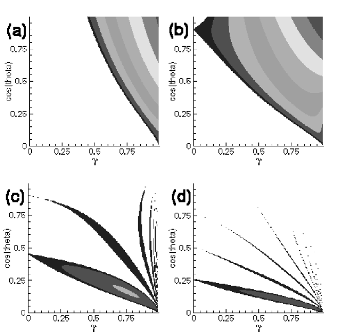
Figure 1: Sample contour plots of instability regimes for $\alpha_{1}=0.5$, $\alpha_{2}=0.3$, $\beta=1.0$, $E_{\omega}=0$ computed on a $250\times 250$ grid for various values of $\Omega$: (a) -0.5, (b) 0, (c) 1.0, and (d) 2.5. Note that the individual fingers touch the $\cos\theta$ axis according to (55).

For nonzero values of $\gamma$, we must investigate the system numerically. We use the variable coefficient ordinary differential equation solver DVODE [30]. The level surface of the growth rate for fixed $\alpha_{1}=0$ is seen in Fig. 2, and Fig. 3 shows the growth rate surface maximized over the $\gamma,\cos\theta$ plane as a function of $\alpha_{1},\alpha_{2}$. Numerical experiments show that $\sigma_{\mathrm{max}}$ has the value associated with the NS equations for $\alpha_{1}=\alpha_{2}=0$. As the parameters $\alpha_{1,2}$ increase, $\sigma_{\mathrm{max}}$ increases to a value of unity on the line $\alpha_{1}\beta^{2}+\alpha_{2}\beta^{4}=1+2\Omega$, and then decreases slowly to zero as $\alpha_{1,2}\to\infty$. This threshold line corresponds to the maximal rate of change of $\sigma_{\mathrm{max}}$ in (59) with respect to $\gamma$. See Fig. 3.

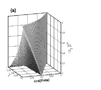
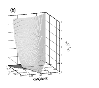
Figure 2: Surface of $\sigma=0.01$ for $E_{\omega}=0$, $\alpha_{1}=0$, $\beta=\sqrt{2}$, $\Omega=0$, and various $\alpha_{2}$. Figure (a) shows the neutral surface for $0\leq\alpha_{2}\leq 0.25$ and is an expansion of the boxed region in figure (b). For $\alpha_{2}=0$, the critical stability point occurs at $\theta=\pi/3$, which agrees with the classical NS results. The critical stability point shifts towards $\cos\theta=1$ as $\alpha_{2}$ increases according to $\cos\theta=(1+\alpha_{2}\beta^{4})/2$. As $\alpha_{2}\beta^{4}$ exceeds unity, a stable band of rotating flows with nonzero eccentricities appears. The corresponding surfaces for $\alpha_{2}=0$ and various $\alpha_{1}$ are qualitatively the same, albeit as a function of $\alpha_{1}\beta^{2}$. See [21].

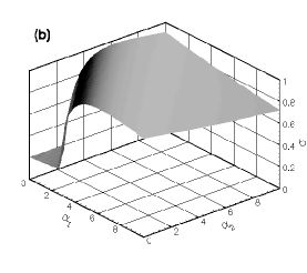
Figure 3: Growth rate surface $\sigma$ maximized over the $\cos\theta,\gamma$ plane as a function of $\alpha_{1}$ and $\alpha_{2}$ for $E_{\omega}=0$, $\beta=1$, (a) $\Omega=0$ and (b) $\Omega=2.5$. In figure (a), the growth rate for $\alpha_{1}=\alpha_{2}=0$ (corresponding to the classic NS case) is $0.36$. We see that the growth rate quickly increases to unity on the line $\alpha_{1}\beta^{2}+\alpha_{2}\beta^{4}=1+2\Omega$ and then slowly decays. Not shown is that $\sigma\to 0$ as $\alpha_{1},\alpha_{2}\to\infty$.

4.2 Viscous results for gradient fluids

The solutions to (49) must be simulated numerically for $E_{\omega}\neq 0$. An interesting feature of this equation is that, unlike the NS equations, a change of variables will not remove viscosity from the problem. However, the qualitative results for NS hold true here. Viscosity stabilizes the flow by lowering the maximum growth rate and introducing a stable band of eccentricities. This stabilization is slower than its NS counterpart, that is, the disspation in (2.1) is of the form $\nu\Delta{\mathbf{u}}$, not $\nu\Delta{\mathbf{v}}$. See Figs. 4 and 5.

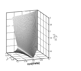
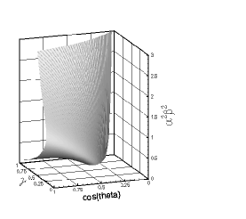
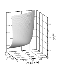
Figure 4: Surface of $\sigma=0.01$ for $\alpha_{2}=0$, $\beta=1$, $\Omega=0$, as functions of $\alpha_{1}$ for (a) $E_{\omega}=0.1$, (b) $E_{\omega}=0.5$, and (c) $E_{\omega}=1.0$, $E_{\omega}=\nu\beta^{2}/|\omega|$. Again, the corresponding surfaces for $\alpha_{1}=0$ and various $\alpha_{2}$ is qualitatively the same. Namely, the unstable region shrinks as viscosity in $E_{\omega}$ increases.

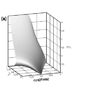
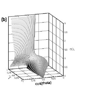
Figure 5: Surface of $\sigma=0.01$ for $\Omega=0$, $\nu/|\omega|=1$ as a function of the wavenumber $\beta$ for (a) $\alpha_{2}=0$, $\alpha_{1}=1$ and (b) $\alpha_{1}=0$, $\alpha_{2}=1$. For $\beta\ll 1$, the flow is inviscid. As $\beta$ increases, the leading order term in an asymptotic exapnsion of (44) will be $-E_{\omega}|{\mathbf{k}}|^{2}{\mathbf{a}}$. Since $E_{\omega}=\nu\beta^{2}/|\omega|$, viscous dissipation quickly takes over.

5 Conclusions

The presence of nonlinear elasticity was seen to have profound effects on the properties of elliptic instability. It can affect the growth rates, as well as the shapes and sizes of the unstable parameter regimes. One of the most profound effects is the thickening of the resonance domains (fingers, or Arnold tongues) in Fig. 1. These resonance domains of instability were predicted for the NS elliptic instability. However, in the NS case, they are infinitesimally thin.

The second gradient fluid constituitive relation and the LANS$-\alpha$ turbulence model both introduce higher derivatives in the momentum density. We found that the highest derivative dominates and produces qualitatively similar effects on the neutral stability surfaces. That is, Fig. 2 shows a similar behavior of the neutral surface as a function of $\alpha_{2}\beta^{4}$ as found for the LANS$-\alpha$ model as a function of $\alpha_{1}\beta^{2}$, in the present notation.

As seen in Fig. 3, first and second gradient fluids increase the Lyapunov growth rates associated with elliptic instability for $\alpha_{1}\beta^{2}+\alpha_{2}\beta^{4}<1+2\Omega$ and then decrease the growth rates for parameter values beyond this threshold. When $\alpha_{2}=0$, this relation recovers the result for LANS$-\alpha$. Thus, the higher-order smoothing due to $\alpha_{2}\neq 0$ comes into play to reduce the maximum growth rate for short waves.

Viscosity has the expected effects on the domain of elliptic instability, as seen in Figs. 4 and 5. However, these effects depend sensitively on the value of $\alpha_{1}$ and $\alpha_{2}$. Figure 5 shows how the effects of nonlinear viscoelasticity depend on the values of $\alpha_{1}$ and $\alpha_{2}$ as a function of the wave number $\beta$. The $\alpha_{2}$ term corresponds to the $\beta^{4}$ dependence, which comes into play very rapidly in its effect on the neutral surface for elliptic instability in Fig. 5b.

Our investigation followed the approach of Fabijonas and Holm [21, 22], who studied the corresponding mean effects of turbulence on elliptic instability for a class of turbulence closure models. For inviscid fluids, the effects of elliptic instability seen in gradient fluids and in the turbulence closure models are qualitatively similar. The inviscid first gradient fluid corresponds to the LANS$-\alpha$ turbulence model, which can be viewed as the nonlinear terms in an LES model for turbulence whose filter is the inverse of the Helmholtz operator $(1-\alpha_{1}\nabla^{2})$ [18]. The inviscid second gradient fluid can be viewed similarly, for which the filter is $(1-\alpha_{1}\nabla^{2}+\alpha_{2}\nabla^{4})^{-1}$, instead.

Future studies may investigate the roles of other aspects of nonlinear stress on elliptic instability, for example, in the Rivlin-Ericksen-Green multipolar fluids analyzed in Bellout et al[11].

References

References

- [1] Eringen A C, ed 1976 Continuum physics: Volume IV Polar and Nonlocal Field Theories (New York: Academic Press)
- [2] Nowacki W 1986 Theory of Asymmetric Elasticity (Oxford: Pergamon Press)
- [3] de Gennes P G and Prost J 1993 The Physics of Liquid Crystals 2nd ed (Oxford:Oxford University Press)
- [4] Holm D D 2002 Euler-Poincaré dynamics of perfect complex fluids, in: Newton P, Holmes P and Weinstein A, eds Geometry, Mechanics, and Dynamics (New York: Springer) 113-68
- [5] Cosserat E and Cosserat F 1909 Théorie des corps deformable (Paris: Hermann)
- [6] Rivlin R S and Erickson J L 1955 J. Rat. Mech. Anal. 4 323–425
- [7] Green A E and Rivlin R S 1964 Arch. Rat. Mech. Anal. 16 325–53
- [8] Green A E and Rivlin R S 1964 Arch. Rat. Mech. Anal. 17 113–47
- [9] Dunn J E and Fosdick R L 1974 Arch. Rat. Mech. Anal. 56 191–252
- [10] Fosdick R L and Rajagopal K R 1980 Proc. R. Soc. Lond. A 339 351–77
- [11] Bellout H, Nećas J and Rajagopal K R 1999 Int. J. Eng. Sci. 37 75–96
- [12] Pierrehumbert R T 1986 Phys. Rev. Lett. 57 2157–9
- [13] Bayly B J 1986 Phys. Rev. Lett. 57 2160–3
- [14] Landman M J and Saffman P G 1987 Phys. Fluids 30 2339–42
- [15] Waleffe F 1990 Phys. Fluids A 2 76–80
- [16] Kerswell R R 2002 Annu. Rev. Fluid Mech. 34 83–113
- [17] Holm D D, Marsden J E and Ratiu T S 1998 Adv. Math. 137 1–81
- [18] Foias C, Holm D D, and Titi E S 2001 Physica 152-3D 505–19
- [19] Rivlin R S 1957 Q. Appl. Math. 15 212
- [20] Craik A D D and Criminale W O 1986 Proc. R. Soc. London A 406 13–26
- [21] Fabijonas B R and Holm D D 2003 Phys. Rev. Lett. 90 124501
- [22] Fabijonas B R and Holm D D 2004 Phys. Fluids 16 853-66
- [23] Foias C, Holm D D and Titi E S 2002 J. Dyn. Diff. Eqns. 14 1–35
- [24] Craik A D D 1989 J. Fluid Mech. 198 275–92
- [25] Miyazaki T 1993 Phys. Fluids 5 2702–09
- [26] Lagnado R R and Simmen J A 1993 J. Non-Newtonian Fluid Mech. 40 29–44
- [27] Goddard J D and Alam M 1999 Part. Sci. Tech. 17 69–96
- [28] Lifschitz A, Miyazaki T and Fabijonas B R 1998 Eur. J. Mech. B/Fluids 17 605–13
- [29] Yakubovich V A and Starzhinskii V M 1967 Linear Differential Equations with Periodic Coefficients (New York: Wiley)
- [30] Brown P, Byrne G and Hindmarsh A 1989 SIAM J. Sci. Stat. Comput. 10 1038–51