Nobility and Stupidity:
Modeling the Evolution of Class Endogamy

Abstract

Class endogamy is a phenomenon in which nobles only marry other nobles and commoners only marry other commoners. The origin of class endogamy, and of social stratification in general, is a major open question in archaeology. This paper implements a verbal model proposed by Marcus and Flannery as a class of agent-based computer models by generalizing and simplifying a mathematical model of marriage markets developed by Burdett and Coles. One force that can produce class endogamy occurs if agents are only willing to marry suitors having status no less than some fixed value below the status of their highest-status suitor, which they can learn. Another such force results if children inherit the average of their parents’ statuses. In contrast, status achieved over an agent’s lifetime can be viewed as noise, analogous to mutation in biological evolution. I propose that class endogamy may have resulted from the interaction of forces such as these, along with other factors such as ideology. Simulation results are presented, and potential areas for future research are sketched out. The validity of these models for any particular culture depends, of course, on whether these forces were actually operating in that society.

1 Introduction

The origin of social inequality is one of the core questions in the social sciences. In archaeology, a related question is the origin of class endogamy, where men and women marry only within their own class. At first glance, this might not seem to need any explanation: Social stratification and class endogamy were widespread in most Western societies until relatively recently. However, many other societies had neither. The question thus arises as to why class endogamy should be present in one society and not in another, and what factors cause it to evolve.

The vast array of human societies have often been classified by anthropologists and archaeologists into several broad categories [31, 29, 10, 8, 9]. While these categories are generalizations that do not necessarily fit all societies well, they are still useful theoretical constructs [9]. In hunter-gatherer bands [15], no one individual is allowed to accumulate significantly more status or wealth than any other. The decisions of a band are collective, with even the most able or experienced members bowing to the group consensus. In tribes [29, 27] or autonomous village societies, an individual is allowed to accumulate wealth and status but must continually expend this wealth in feasts or as gifts in order to maintain that status. A big man is a member of a tribe who has accumulated enough status to be able to mobilize others to action; however, a big man may be deposed if he demands too much or fails to provide enough gifts. In these societies, an individual’s possessions are often destroyed after death, and children do not inherit their parents’ status. In chiefdoms [5, 16] or rank societies, wealth and rank can be inherited at birth, along with whatever individuals accumulate in their own lifetimes. However, all members of the society are considered to be at least distantly related to one another, and rank is continuous: There is no chiefly or noble class. These societies are ruled by a chief who can command others by virtue of his office alone, and the office may be hereditary. While the chief may have a group of lieutenants, they have no specialized functions. In contrast, in a complex chiefdom [6, 35] or stratified society, there is a “discontinuity in rank between chiefs and commoners” [6, p. 12]: The chiefs are no longer related to the lowest-ranking members of society, and their close relatives constitute a chiefly or noble class, who practice class endogamy. In addition, the chief’s lieutenants now have specialized roles in the government. Finally, in a state [29, 30, 8, 34, 5], features such as a specialized bureaucracy and a standing professional army arise.

Assuming that the first human societies were small, egalitarian bands of hunter-gatherers [9], a major question in archaeology is why sedentary agricultural societies emerged, with rank differences or even stratification into classes. Hunter-gatherers generally appear to have more leisure time and less disease than sedentary farmers, and it seems against human nature to voluntarily give a portion of one’s production to a “macroparasite” [22] such as a chief or king. Even if sedentism, agriculture, and rank differences between individuals are explained, there remains the question of how stratification into classes of nobles and commoners arose. These questions are important if we want to understand contemporary human societies, as well as how they came to be.

This paper attempts to address the question: Given a chiefdom where individuals both inherit status at birth and also achieve or lose status over their lifetimes, what are the necessary and sufficient conditions for a stratified society with class endogamy to arise? More specifically, what is the simplest class of agent-based computer models [28, 26, 25, 18, 19, 17, 7, 1, 13] that produce a result qualitatively identical to class endogamy, given a plausible set of assumptions? How rational must the modeled individuals be to form classes of nobles and commoners? In other words, how stupid can the agents be and still produce class endogamy?

Following Wright [35, p. 68], I define a noble class as “a ranked group whose members [compete] with each other for access to controlling positions and stand together in opposition to other people”. For the purposes of these computer models, however, a class will simply be a set of men and a set of women, each from contiguous status intervals, who practice endogamy: Most of the time, they marry only each other.

I will show that one force that can produce class endogamy occurs if agents are only willing to marry suitors having status no less than some fixed value below the status of their highest-status suitor. Furthermore, agents can easily learn what the status of their highest-status suitor is. Another such force results if children inherit the average of their parents’ statuses. In contrast, status achieved over an agent’s lifetime can be viewed as noise, analogous to mutation in biological evolution. I propose that class endogamy may have been produced by the interaction of forces such as these, along with other factors such as ideology [35]. Whether these models have any bearing on how class endogamy actually evolved in any particular human society must of course be tested against the ethnographic, ethnohistorical, archaeological, and psychological data. However, such testing is beyond the scope of this paper.

The paper is organized as follows: This section has laid out the background and the question. The next section, Section 2, introduces a verbal model from archaeology that has been proposed to explain the evolution of class endogamy. Section 3 describes a mathematical model from economics that will be generalized and simplified to implement this verbal model as a class of agent-based computer models, which are presented in Section 4, along with their results. Section 5 summarizes the paper, and Section 6 outlines some avenues for future research.

2 A Verbal Model from Archaeology

My starting point for this paper is a verbal model of the emergence of class endogamy proposed by Marcus and Flannery:

In most chiefdoms, there is a continuum of differences in rank from top to bottom. People are ranked in terms of their genealogical distance from the paramount chief, with the lowliest persons being very distantly related indeed. In most archaic states, there was an actual genealogical gap between the stratum of nobles and the stratum of commoners. Lesser nobles knew they were at least distantly related to the king. Commoners were not considered related to him at all. As we have seen, the two strata were kept separate by class endogamy, the practice of marrying within one’s class.

There are many possible scenarios for the evolution of stratified society out of chiefly society. An actor-centered explanation might begin with a chief’s need to ensure that his offspring would succeed him. The only way he could ensure that goal was by marrying the highest-ranking woman available. The genealogical gap mentioned earlier could arise through intense competition for the most advantageous marriages. Eventually the more genealogically distant members of society — marriage to whom would only condemn one’s offspring to lower rank — might have their kin ties to the elite severed. This apparently happened to low-ranking families in Hawaii just prior to state formation.[21, p. 181]

The main goals of this paper are to explore how to implement Marcus and Flannery’s verbal model as a class of agent-based computer models and to examine whether they in fact produce class endogamy as expected. Computer models have the virtue that the outcomes follow rigorously from the model’s assumptions. Furthermore, the model’s assumptions and mechanisms must be specified explicitly.

Specifically, my goal is to find the simplest class of agent-based computer models that produce class endogamy, starting with a simple ranked society. In contrast to many computer simulations in the archaeological and anthropological literature, I do not attempt to include every feature that appears to be relevant; rather, my goal is to include the minimal set of features necessary and sufficient to produce class endogamy. I do this for several reasons: First, following Occam’s razor, it makes little sense to design a complicated model when a simpler model suffices. Second, a simple model is easier to implement and debug than a complicated one. Finally, a simple model produces results that are easier to understand. If the model were as complicated as the real system, the results would be much more realistic than a simple model, but just as hard to understand as the real world.

In this paper, I also make no attempt to incorporate empirical data such as status distributions from real societies. While such data would be valuable for the validation of the model for any particular society, in this paper I have adopted a data-independent approach, in order to construct a general class of models. Any empirical data that might be incorporated would be at least partially incorrect, especially for societies that no longer exist. A model that held for all possible status distributions would obviously be inherently more general and reliable than one constructed under the assumption of any specific “real” status distribution. Any illusion of support given by such data would be outweighed by the risk that the data were in fact wrong, since in that case, a model built around that data could be fatally flawed. Of course, once a class of general, data-independent models has been developed, any empirical data that are available can and should be used to test whether the models are applicable to a particular society. Such testing is beyond the scope of this paper, however.

As Renfrew writes concerning modeling in archaeology,

…[A]ny models which we may set up are likely to be over simplified, but I believe the effort is worthwhile. For it then allows us, when considering any specific case of change, to refer it back to the general models which we have, and to see if they are of help in explaining what has been observed. In many cases I believe that they are. This undertaking of attempting some sort of explanation through generalization is what is termed in contemporary archaeology the processual approach. It has the merit of making our explanations explicit, which is a very effective way of bringing their weaknesses to light, and hence also of investigating their strengths. [24, pp. 120–121]

3 A Mathematical Model from Economics

How might Marcus and Flannery’s model be implemented on a computer, and how exactly might class endogamy emerge from agents competing for high-status spouses? One possible source of answers for these questions is economics, where much work has been done to model marriage markets and the related domain of labor markets. In particular, Burdett and Coles [3] have shown mathematically that classes emerge endogenously in a marriage market given certain assumptions. They considered a population of agents that decide whether to marry one another based on their respective “pizazz”, or desirability, which is modeled as a real number. The utility an agent receives from a marriage is equal to its spouse’s pizazz, discounted according to how long it had to wait before marrying. Burdett and Coles assume that the agents try to maximize their utility, and that they know the rate at which they meet agents of the opposite sex, as well as the distribution of pizazz for those agents. Under these assumptions, they show that an equilibrium exists, in which each agent will use a strategy to maximize its expected discounted lifetime utility by only proposing to agents who have pizazz equal to or greater than this expected utility, which can be calculated. Furthermore, endogamy emerges: The individuals partition themselves into discrete groups, where the males and females are each divided into contiguous intervals of pizazz, and females will only marry males from the same group, and vice versa. In a second paper [4], they extended their model to consider the effect of self-improvement, i.e., pizazz that an agent can achieve at some cost during its lifetime. Endogamy also emerges in this second model, and they prove results concerning the amount of self-improvement a given agent will choose to invest in.

If status is substituted for pizazz, and achieved status for self-improvement, then these results can be transfered directly to the question of how class endogamy emerged in past societies. Furthermore, this mathematical model could be directly implemented on a computer, since each agent’s optimal strategy can be calculated. Hence, Burdett and Coles have provided one possible operationalization of Marcus and Flannery’s verbal model and verified it mathematically, within the context of their assumptions.

This is a significant and interesting result. However, Burdett and Coles implicitly assume that, in order to determine who they should propose to, agents are able to calculate which agents are willing to marry them, the rate at which they encounter such agents, and the pizazz distribution of those agents. Anecdotal evidence from contemporary American society gives us some reason to doubt that men and women actually know this information in general (though it might in fact be true for the relatively simple, low-population societies we are considering in this paper). Furthermore, their model presumes that agents calculate an optimal strategy; while this allows them to prove that an equilibrium exists, it begs the question of whether such optimal strategies are actually necessary to produce endogamy. Are there other strategies that produce the same effect? Why exactly does this type of strategy produce endogamy? And in particular, are there simple heuristics that also result in endogamy? Can the agents be made less rational, i.e., more stupid? The next section generalizes and simplifies Burdett and Coles’s proof in order to answer these questions.

3.1 Burdett and Coles’s Proof, Generalized and Simplified

Suppose that agents with status $s$ will only marry suitors with status $s^{\prime}\geq s^{\prime}_{\mathrm{max}}(s)-f(H(s)),$ where $s^{\prime}_{\mathrm{max}}(s)$ is the status of the highest-status agent willing to marry an agent with status $s,$ and $f(H(s))\geq 0$ is some function of the distribution of status $H(s)$ among those willing to marry an agent with status $s.$ This section will prove that, under those circumstances, class endogamy results.

This proof relies on the following assumptions regarding status: First, females all use a single, uniform status metric to evaluate male suitors, and vice versa. Second, the status of any two agents can be compared, and these comparisons are transitive, i.e., $s(a_{1})\geq s(a_{2})\wedge s(a_{2})\geq s(a_{3})\Rightarrow s(a_{1})\geq s(a_{3}),$ where $s(a_{i})$ is the status of agent $a_{i},$ represented by a real number. Third, agents are always willing to marry the highest-status agent willing to marry them. Fourth, all males will propose to the highest-status female, with status $s_{\mathrm{max}}^{\mathrm{f}},$ and all females will propose to the highest-status male, with status $s_{\mathrm{max}}^{\mathrm{m}}.$ Fifth, if an agent is willing to marry a suitor with a given status, then it is willing to marry all higher-status suitors: $M(a_{1},a_{2})\wedge s(a_{2})\leq s(a_{3})\Rightarrow M(a_{1},a_{3}),$ where $M(a_{i},a_{j})$ is true if and only if an agent $a_{i}$ is willing to marry suitor $a_{j}.$ Finally, the threshold for accepting a suitor is nondecreasing with increasing status: $M(a_{1},a_{3})\wedge s(a_{1})\geq s(a_{2})\Rightarrow M(a_{2},a_{3}).$ (This may seem to be a large number of assumptions to make; however, they are all plausible statements about the way status operates.)

The proof is as follows: All males will propose to the highest-status female, with status $s_{\mathrm{max}}^{\mathrm{f}}.$ This female, in turn, will propose to the highest-status male, with status $s_{\mathrm{max}}^{\mathrm{m}},$ as well as to all other males who have status $s^{\prime}\geq s_{\mathrm{max}}^{\mathrm{m}}-f(H(s_{\mathrm{max}}^{\mathrm{f}})).$ Now, since the highest-status female will propose to these males, all females will propose to them. Hence, these males all face the same situation as the highest-status male and will all follow the same strategy. Call this set of males $C_{1}^{\mathrm{m}}.$ They are all willing to accept the highest-status female, along with all other females with status $s^{\prime}\geq s_{\mathrm{max}}^{\mathrm{f}}-f(H(s_{\mathrm{max}}^{\mathrm{m}})).$ Call that set of females $C_{1}^{\mathrm{f}}.$ Those females, in turn, all face the same situation as the highest-status female and thus use the same strategy as she does: Propose only to the males in $C_{1}^{\mathrm{m}}.$ Thus, the females in $C_{1}^{\mathrm{f}}$ will marry only the males in $C_{1}^{\mathrm{m}},$ and vice versa. $C_{1}^{\mathrm{f}}$ and $C_{1}^{\mathrm{m}}$ form a class $C_{1},$ which constitutes the highest social stratum. Figure 1 shows the argument graphically.

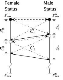
Figure 1: Class formation under the proof in Section 3.1. The highest-status female and male, with selectivity constants $\epsilon^{\mathrm{f}}_{1}=f^{\mathrm{f}}(H(s_{\mathrm{max}}^{\mathrm{f}}))$ and $\epsilon^{\mathrm{m}}_{1}=f^{\mathrm{m}}(H(s_{\mathrm{max}}^{\mathrm{m}})),$ respectively, are represented by solid black circles. The dashed lines indicate the agents that the highest-status female and male are willing to marry, respectively. All males and females between the first two horizontal solid black lines form the first class $C_{1}$ and only marry each other. The highest-status female and male outside of $C_{1}$ are represented by white circles and have selectivity constants $\epsilon^{\mathrm{f}}_{2}$ and $\epsilon^{\mathrm{m}}_{2}.$ All agents between the second set of horizontal solid lines form class $C_{2}.$ The remaining classes are not shown.

To form the next highest class $C_{2},$ remove the individuals in $C_{1}$ from the population and apply the same reasoning, starting with the new highest-status female and male, producing $C_{2}^{\mathrm{f}}$ and $C_{2}^{\mathrm{m}},$ which together constitute $C_{2}.$ Repeat this procedure, forming classes until there are either no females or no males remaining. Note that it is possible for one of the sexes to have one more class than the other, in which case the members of that lowest class will not be able to find anyone willing to marry them.

This generalization of Burdett and Coles’s proof shows that the fundamental mechanisms underlying this form of class endogamy are first, that the agents all decide whether or not to marry a suitor based on its status relative to the status of the highest-status agent willing to marry them, and secondly, that there is an upper bound on status. The function $f(H(s))$ determines how selective an agent is. The rational strategy derived by Burdett and Coles, where agents maximize their expected discounted lifetime utility, is thus a special case of this more general result. (However, their result is more general in the sense that it considers discounting.) In fact, for class endogamy to emerge, it suffices if $f(H(s))=\epsilon,$ where $\epsilon$ is a non-negative integer constant; thus it is not necessary for the agents to know anything about $H(s)$ other than $s^{\prime}_{\mathrm{max}}(s).$ The proof still holds if males and females have different selectivity functions $f^{\mathrm{m}}(H(s))$ and $f^{\mathrm{f}}(H(s)).$ Note also that it does not depend on the particular status distribution in the society. (Furthermore, it is interesting to note that it actually does not depend on the fact that there are sexes at all: The results would still hold if the agents were hermaphroditic.) The proof also provides a procedure for calculating the class boundaries, as well as the highest-status suitor for any given agent.

This generalized strategy is not necessarily optimal; hence, unlike Burdett and Coles, I have not shown that an equilibrium exists in which rational agents will all converge to using this strategy. However, if a population of agents do all use this strategy, then class endogamy will result. In an unstratified simple chiefdom, such as is assumed in these models, it seems plausible to assume that the agents are undifferentiated and will all use the same strategy. The next section introduces a class of agent-based computer models to verify these results.

4 A Class of Computer Models

The basic modeling framework, adapted from Burdett and Coles [3, 4], consists of a population of agents, representing a chiefdom or village. Each agent can be male or female and has an integer status that determines its rank within the society. Part of this status is inherited at birth, and part may be achieved (or lost) over the agent’s lifetime. The population is initialized with some number of agents, with each agent’s inherited status drawn randomly from a uniform distribution. At each time step thereafter, one randomly-chosen female encounters one randomly-chosen male. If both agents find the other acceptable, based on their respective statuses, they marry and produce a pair of children. The parents are removed from the population, and the children are added to it. However, if at least one of the agents rejects the other, they do not marry but instead remain in the population. This cycle continues until some predetermined number of marriages has occurred. The agents live forever, until they marry, and they do not become less selective the longer they remain single — there is no discounting.

In these models, the population was initialized with $N=10,000$ agents, where each agent had a 50% chance of being male or female, and each one had an inherited status $s_{\mathrm{i}}$ drawn from a uniform probability distribution between $s_{\mathrm{min}}=0$ and $s_{\mathrm{max}}=99.$ The models ran until $t_{\mathrm{max}}=100,000$ marriages had occurred. Fifty runs of each model were performed, each run initialized with a different random number seed.

4.1 Cloned Offspring

To keep things simple, agents in the first set of models did not have any achieved status. If a female agent encountered a male agent and both agreed to marry, each parent produced a clone with the same sex and status, and the parents were removed from the population. The distributions of sex and status in the population thus remained constant over time.

4.1.1 Strategy $\mathbf{S}_{1}$: Rationality

I have already shown mathematically in Section 3.1 that class endogamy results if agents all follow a strategy $\mathbf{S}_{1}$ of only accepting suitors who have a status $s^{\prime}\geq s^{\prime}_{\mathrm{max}}(s)-\epsilon,$ where $s^{\prime}_{\mathrm{max}}(s)$ is the status of the highest-status agent willing to marry an agent with status $s,$ and $\epsilon$ is some non-negative integer. In this section, I verify this result using an agent-based computer model, model $\mathbf{M}_{1}.$ When a female agent encountered a male agent in this model, both used strategy $\mathbf{S}_{1},$ with $\epsilon=9.$

Every $10,000$ marriages, the number of males and females at each status level were recorded. The female and male status histograms from a single typical run are plotted at $t=0$ marriages in Figure 2; the distributions remain constant over the entire run.

In addition, the marriage frequencies over the previous $10,000$ marriages were recorded for each combination of female status and male status. These statistics were calculated every $10,000$ marriages, beginning at $t=10,000$ marriages. This is plotted for a single typical run at $t=10,000$ marriages in Figure 3(a); the plots at other sample times are very similar. In these plots, darker points represent more marriages than lighter ones. (The frequency data were scaled logarithmically before plotting, to increase the plots’ legibility.)

To help analyze the marriage frequency data, a hypergamy metric, $h,$ was also calculated every $10,000$ marriages. Hypergamy is a situation in which an individual marries someone of higher status. The opposite situation, where an individual marries someone of lower status, is called hypogamy. The metric $h$ is defined as follows:

$$h(s,t)=\frac{m_{+}(s,t)-m_{-}(s,t)}{m_{+}(s,t)+m_{-}(s,t)+m_{=}(s,t)},$$ (1)

where

$$m_{+}(s,t)=\sum_{t^{\prime}=t-\Delta t}^{t}\>\sum_{i=s+1}^{s_{\mathrm{max}}}m_{s,i}(t^{\prime})$$ (2)

is the number of hypergamous marriages for agents with status $s$ over the sampling period ending at time $t,$

$$m_{-}(s,t)=\sum_{t^{\prime}=t-\Delta t}^{t}\>\sum_{i=s_{\mathrm{min}}}^{s-1}m_{s,i}(t^{\prime})$$ (3)

is the number of hypogamous marriages for those agents over the same period, and

$$m_{=}(s,t)=\sum_{t^{\prime}=t-\Delta t}^{t}m_{s,s}(t^{\prime})$$ (4)

is the number of marriages with agents of equal status. In these equations, $s$ is an individual’s status, $t$ is the number of marriages that have elapsed, $\Delta t=10,000$ is the sampling interval, $s_{\mathrm{min}}$ and $s_{\mathrm{max}}$ are the minimum and maximum possible statuses, respectively, and $m_{i,j}(t)$ is the number of individuals of either sex having status $i$ and $j$ that married at time $t$. The hypergamy metric $h$ ranges between $1$ and $-1.$ If individuals with status $s$ have only hypergamous marriages, i.e., they marry only individuals with higher status, then $h(s)=1;$ conversely, if the individuals have only hypogamous marriages, then $h(s)=-1.$ If the number of hypergamous marriages equals the number of hypogamous marriages, or if the individuals only marry individuals with exactly the same status $s,$ then $h(s)=0.$ This value $h$ is plotted for each status level in Figure 3(b), for a single typical run, and in Figure 3(c) for all $50$ runs, to show the variation between runs. (If no marriages occurred for a given status level, $h$ is undefined, and that point is simply skipped.)

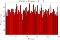
(a) Female status histogram, for one run

(b) Male status histogram, for one run

Figure 2: Female and male status histograms for one typical run at $t=0$ marriages, for the model $\mathbf{M}_{1}$ from Section 4.1.1, using the rational strategy $\mathbf{S}_{1}.$ Children were clones of their parents, and agents did not achieve any status over their lifetimes. Thus, the histogram remained constant over the entire run. The status histograms for the other models at $t=0$ were very similar.

(a) Marriage frequency,
for one run

(b) Hypergamy $h,$ for one run

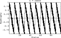
(c) Hypergamy $h,$ for 50 runs

(d) Female status histogram, for one run

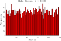
(e) Male status histogram, for one run

Figure 3: Marriage frequency, hypergamy $h,$ and status histograms at $t=10,000$ marriages, for the model $\mathbf{M}_{1}$ from Section 4.1.1, using the rational strategy $\mathbf{S}_{1}.$ Children were clones of their parents, and agents did not achieve any status over their lifetimes. These plots changed very little at later timesteps. The status histograms remained constant over the entire run.

This hypergamy metric $h$ can be used as a proxy for measuring the degree of class endogamy: If the hypergamy changes quickly from a low value to a high value as $s$ increases, then class endogamy is present. The points at which these transitions occur represent class boundaries. (The high values of $h$ near $s_{\mathrm{min}}=0$ and the low values near $s_{\mathrm{max}}=99$ are artifacts of the boundary conditions at these points.) The metric does not work well as a proxy for endogamy when the number of status levels in a class is very close to $1,$ as will be evident later in Section 4.2.

As can be seen in Figure 3, classes emerge immediately when agents all use strategy $\mathbf{S}_{1},$ as expected. This model produces $10$ classes when $\epsilon=9$, while archaic stratified societies probably only had two classes, in general: nobles and commoners [9]. This might seem to invalidate the model; however it can be easily modified to produce only two classes: Simply set $\epsilon=(s_{\mathrm{max}}-s_{\mathrm{min}}+1)/2-1=49.$ Producing $10$ classes is, in fact, a more rigorous test of the model than merely producing two would be. In general, set $\epsilon=(s_{\mathrm{max}}-s_{\mathrm{min}}+1)/n-1,$ where $n$ is the number of classes.

This simulation merely verifies what was already proven mathematically in Section 3.1. Furthermore, strategy $\mathbf{S}_{1}$ is less than satisfying, since in order for an agent to calculate the highest-status agent willing to marry it, it must first calculate what class it lies in, using the procedure from the proof in Section 3.1. Hence, the agents are in essence forming classes by calculating a priori what class they are in. (The same applies to Burdett and Coles’s model [3, 4].) Is it possible for the agents to learn what the highest-status agent willing to marry them is, so that classes emerge without such calculations? If so, this circularity could be broken.

4.1.2 Strategy $\mathbf{S}_{2}$: Learning

The goal for this section is to show that there is a simple algorithm $\mathbf{S}_{2}$ that agents can use to learn the status of the highest-status agent willing to marry them. Once such an algorithm was found, no effort was made to improve on it or analyze it in detail; this is merely an existence proof that such learning is possible. A simpler or more efficient algorithm may well exist. The algorithm is as follows: For each status level $s,$ keep a list of the last $n_{\mathrm{e}}$ encounters that females with status $s$ experienced with males, along with their outcomes. Keep a similar set of lists of males’ encounters with females. Initially, no encounters have occurred, and the lists are empty. Every time an encounter occurs, update the appropriate male and female encounter lists. If $n_{\mathrm{e}}$ encounters have already been recorded for a given status and sex, then remove the oldest encounter before adding the most recent one to the list. If the encounter list corresponding to an agent’s status $s$ is not full, the agent uses strategy $\mathbf{S}_{3}$: Only accept suitors that have status at least equal to $s-\epsilon,$ where $s$ is the agent’s own status, and $\epsilon$ is some non-negative integer. This implicitly defines an interval with radius $\epsilon$ around an agent’s status $s,$ encompassing the agent’s potential mates. (Note that strategy $\mathbf{S}_{3}$ requires that males and females both use the same status scale $[s_{\mathrm{min}},s_{\mathrm{max}}]$ to evaluate the opposite sex.) Once an agent’s encounter list is full, it switches to strategy $\mathbf{S}_{1},$ described in Section 4.1.1, where $s^{\prime}_{\mathrm{max}}(s)$ is defined to be the status of the highest-status agent of the opposite sex that was willing to marry an agent with status $s$ within the last $n_{\mathrm{e}}$ encounters. In these simulations, $n_{\mathrm{e}}=2(s_{\mathrm{max}}-s_{\mathrm{min}}+1)=200$ and $\epsilon=9.$

Model $\mathbf{M}_{1}$ from Section 4.1.1 was modified to use the learning strategy $\mathbf{S}_{2},$ producing model $\mathbf{M}_{2}.$ The same marriage frequency, hypergamy, and status data were recorded as in Section 4.1.1, and these are plotted in Figures 4–5 at $t=10,000$ and $t=20,000$ marriages. (These plots changed very little after $20,000$ marriages.) The male and female status histograms were constant during the entire run.

Class formation proceeds quickly in this model, with the highest-status class evident after only $10,000$ marriages and others forming within $20,000$ marriages; however it also stagnates quickly after this point: Only about five clearly-defined classes formed, even after $100,000$ marriages had occurred, compared with $10$ classes in model $\mathbf{M}_{1}$ under the rational strategy $\mathbf{S}_{1}.$ Archaic societies probably only had two classes, nobles and commoners [9]; hence, this does not seem to be a severe limitation of the model. (Note that class formation is initiated among the highest-status agents and moves down along the status scale, just as in the proof in Section 3.1.) Thus, it is indeed easy for agents to learn $s^{\prime}_{\mathrm{max}}(s).$ However, the efficiency of this particular learning algorithm may depend on the status distribution in the population, as well as the population size. These factors are not investigated in this paper.

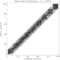
(a) Marriage frequency,
for one run

(b) Hypergamy $h,$ for one run

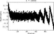
(c) Hypergamy $h,$ for 50 runs

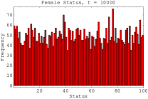
(d) Female status histogram, for one run

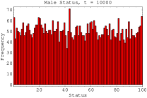
(e) Male status histogram, for one run

Figure 4: Marriage frequency, hypergamy $h,$ and status histograms at $t=10,000$ marriages, for the model $\mathbf{M}_{2}$ from Section 4.1.2, using the learning algorithm $\mathbf{S}_{2}.$ Children were clones of their parents, and agents did not achieve any status over their lifetimes.

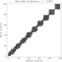
(a) Marriage frequency,
for one run

(b) Hypergamy $h,$ for one run

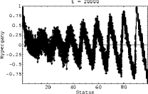
(c) Hypergamy $h,$ for 50 runs

(d) Female status histogram, for one run

(e) Male status histogram, for one run

Figure 5: Marriage frequency, hypergamy $h,$ and status histograms at $t=20,000$ marriages, for the model $\mathbf{M}_{2}$ from Section 4.1.2, using the learning algorithm $\mathbf{S}_{2}.$ Children were clones of their parents, and agents did not achieve any status over their lifetimes. These plots remained very similar at later timesteps in the runs. The status histograms remained constant.

In a real chiefdom, agents would not be starting with a blank slate at $t=0$ and would always have a history of past marriages to consult. Thus, the initialization period required in this model, where the agents use the interval around self strategy $\mathbf{S}_{3}$ before switching to the rational strategy $\mathbf{S}_{1},$ is an artifact of the model itself.

4.1.3 Strategy $\mathbf{S}_{3}$: Interval Around Self

Another plausible scenario would be for all of the agents to simply use the strategy $\mathbf{S}_{3}$ described in Section 4.1.2, with $\epsilon=9.$ This is a sort of null hypothesis, $\mathbf{S}_{3}$ being the simplest possible strategy that takes a suitor’s status into consideration, relative to the agent’s own. Does this strategy also produce class endogamy? The model $\mathbf{M}_{1}$ from Section 4.1.1 was modified to use strategy $\mathbf{S}_{3},$ producing model $\mathbf{M}_{3},$ and the results are plotted in Figure 6 at $t=100,000$ marriages. As before, the male and female status histograms remain constant over the entire run. As can be seen, the married couples are strongly correlated according to status, but no class endogamy occurs within $100,000$ marriages under this strategy: Strategy $\mathbf{S}_{3}$ by itself is not a mechanism for producing class endogamy. Something further is needed.

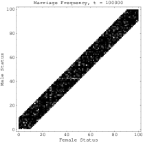
(a) Marriage frequency,
for one run

(b) Hypergamy $h,$ for one run

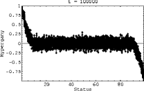
(c) Hypergamy $h,$ for 50 runs

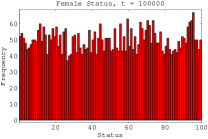
(d) Female status histogram, for one run

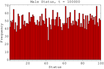
(e) Male status histogram, for one run

Figure 6: Marriage frequency, hypergamy $h,$ and status histograms at $t=100,000$ marriages, for the model $\mathbf{M}_{3}$ from Section 4.1.3, using the interval around self strategy $\mathbf{S}_{3}.$ Children were clones of their parents, and agents did not achieve any status over their lifetimes. These plots were very similar at all timesteps during the runs. The status histograms were constant throughout the run.

4.2 Inherited Status

In the previous models, a child was simply the clone of one of its parents. What happens if status is inherited from both parents? One plausible type of inheritance is for both children simply to receive the average of their parents’ overall statuses. This has the virtue that a high-status agent’s offspring have a lower status if it marries a low-status agent; conversely, a low-status agent who marries a high-status agent has the status of its offspring raised. For example, Kirch [16, pp. 31–36] writes that in Polynesian chiefdoms, each person was ranked primarily according to his or her genealogical distance from the founding ancestor, along the paternal line. However, rank could also be transmitted along the maternal line, and females outranked males in some cases. Thus, males could increase the status of their offspring by marrying high-status females.

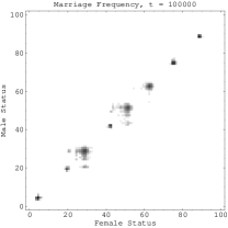
(a) Marriage frequency,
for one run

(b) Hypergamy $h,$ for one run

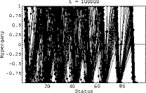
(c) Hypergamy $h,$ for 50 runs

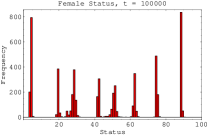
(d) Female status histogram, for one run

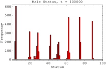
(e) Male status histogram, for one run

Figure 13: Marriage frequency, hypergamy $h,$ and status histograms at $t=100,000$ marriages, for the model $\mathbf{M}_{5}$ from Section 4.2, using the learning algorithm $\mathbf{S}_{2}.$ Children inherited the average of their parents’ statuses, and agents did not achieve any status over their lifetimes.

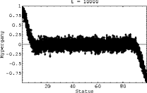
(c) Hypergamy $h,$ for 50 runs

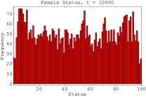
(d) Female status histogram, for one run

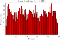
(e) Male status histogram, for one run

Figure 14: Marriage frequency, hypergamy $h,$ and status histograms at $t=10,000$ marriages, for the model $\mathbf{M}_{6}$ from Section 4.2, using the interval around self strategy $\mathbf{S}_{3}.$ Children inherited the average of their parents’ statuses, and agents did not achieve any status over their lifetimes.

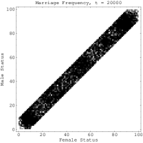
(a) Marriage frequency,
for one run

(b) Hypergamy $h,$ for one run

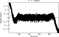
(c) Hypergamy $h,$ for 50 runs

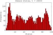
(d) Female status histogram, for one run

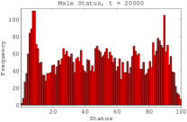
(e) Male status histogram, for one run

Figure 15: Marriage frequency, hypergamy $h,$ and status histograms at $t=20,000$ marriages, for the model $\mathbf{M}_{6}$ from Section 4.2, using the interval around self strategy $\mathbf{S}_{3}.$ Children inherited the average of their parents’ statuses, and agents did not achieve any status over their lifetimes.

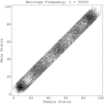
(a) Marriage frequency,
for one run

(b) Hypergamy $h,$ for one run

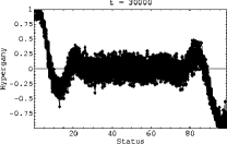
(c) Hypergamy $h,$ for 50 runs

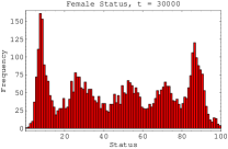
(d) Female status histogram, for one run

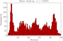
(e) Male status histogram, for one run

Figure 16: Marriage frequency, hypergamy $h,$ and status histograms at $t=30,000$ marriages, for the model $\mathbf{M}_{6}$ from Section 4.2, using the interval around self strategy $\mathbf{S}_{3}.$ Children inherited the average of their parents’ statuses, and agents did not achieve any status over their lifetimes.

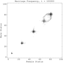
(a) Marriage frequency,
for one run

(b) Hypergamy $h,$ for one run

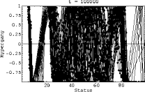
(c) Hypergamy $h,$ for 50 runs

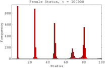
(d) Female status histogram, for one run

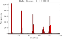
(e) Male status histogram, for one run

Figure 17: Marriage frequency, hypergamy $h,$ and status histograms at $t=100,000$ marriages, for the model $\mathbf{M}_{6}$ from Section 4.2, using the interval around self strategy $\mathbf{S}_{3}.$ Children inherited the average of their parents’ statuses, and agents did not achieve any status over their lifetimes.

Each of the previous computer models $\mathbf{M}_{1},\mathbf{M}_{2},$ and $\mathbf{M}_{3}$ was modified to use this form of inheritance, with children’s sex determined randomly, producing a new set of models $\mathbf{M}_{4},\mathbf{M}_{5},$ and $\mathbf{M}_{6}.$ The results are shown in Figures 7–9 for model $\mathbf{M}_{4}$ using the rational strategy $\mathbf{S}_{1}$ from Section 4.1.1, Figures 10–13 for model $\mathbf{M}_{5}$ using the learning algorithm $\mathbf{S}_{2}$ from Section 4.1.2, and Figures 14–17 for model $\mathbf{M}_{6}$ using the interval strategy $\mathbf{S}_{3}$ from Section 4.1.3. Note that the hypergamy metric $h$ breaks down as a proxy for measuring class endogamy when the peaks in the status histogram become very narrow, as shown in Figure 9. This is because $h=0$ at many points, or is undefined, reducing the size of the jumps from low $h$ to high $h,$ despite the fact that the degree of class endogamy is very high.

Under all three strategies, this form of inherited status has the effect of converting a uniform status distribution into a multimodal one, with peaks and valleys in the status histogram. Over long time periods, gaps in the status distribution appear, in which there are very few agents having a given status level, or none at all.

The multimodality and gaps in the status distribution are caused by a kind of regression towards the mean: A child’s expected status lies in the middle of an endogamous class. Thus, the class boundaries move inwards over time. Even under strategy $\mathbf{S}_{3}$ in model $\mathbf{M}_{6},$ this effect alone is strong enough to produce class endogamy: Gaps appear in the status distribution after about $30,000$ marriages, reducing agents’ marriage options outside of the local peak in the status histogram. This seems to be driven by the fact that the highest- and lowest-status individuals are constrained to find spouses within intervals $\epsilon$ lower and higher than them, respectively. These constraints produce sufficient class boundaries for the regression effect to produce gaps in the status histogram. This effect seems to be very similar to the segregation phenomenon investigated by Weisbuch and coworkers [32], in their simplest model. Although they do not provide an explanation for this phenomenon, they do show that the number of clusters formed is generally equal to $\lfloor 100/(2(\epsilon+1))\rfloor$ (translated into the parameters used here). This prediction seems to be borne out in model $\mathbf{M}_{6},$ since the number of classes formed by the end of a run tends to be $\lfloor 100/(2(9+1))\rfloor=5,$ as can be seen in Figure 17(a). This model may also have some similarities with Axelrod’s culture diffusion model [2], in which a lattice of villages coalesces into a few discrete “cultures”.

In general, averaging inheritance increases the degree of class endogamy under all three strategies. Hence, this type of inheritance is another force that can produce class endogamy. (If children inherited a weighted average of their parents’ statuses, this force would still drive the model towards class endogamy, though less strongly.)

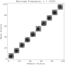
(a) Marriage frequency,
for one run

(b) Hypergamy $h,$ for one run

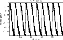
(c) Hypergamy $h,$ for 50 runs

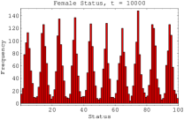
(d) Female status histogram, for one run

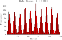
(e) Male status histogram, for one run

Figure 7: Marriage frequency, hypergamy $h,$ and status histograms at $t=10,000$ marriages, for the model $\mathbf{M}_{4}$ from Section 4.2, using the rational strategy $\mathbf{S}_{1}.$ Children inherited the average of their parents’ statuses, and agents did not achieve any status over their lifetimes.

(a) Marriage frequency,
for one run

(b) Hypergamy $h,$ for one run

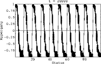
(c) Hypergamy $h,$ for 50 runs

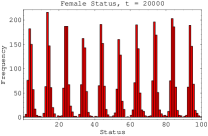
(d) Female status histogram, for one run

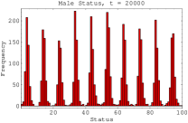
(e) Male status histogram, for one run

Figure 8: Marriage frequency, hypergamy $h,$ and status histograms at $t=20,000$ marriages, for the model $\mathbf{M}_{4}$ from Section 4.2, using the rational strategy $\mathbf{S}_{1}.$ Children inherited the average of their parents’ statuses, and agents did not achieve any status over their lifetimes.

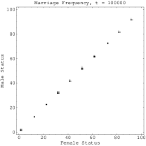
(a) Marriage frequency,
for one run

(b) Hypergamy $h,$ for one run

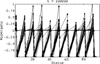
(c) Hypergamy $h,$ for 50 runs

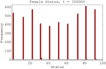
(d) Female status histogram, for one run

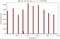
(e) Male status histogram, for one run

Figure 9: Marriage frequency, hypergamy $h,$ and status histograms at $t=100,000$ marriages, for the model $\mathbf{M}_{4}$ from Section 4.2, using the rational strategy $\mathbf{S}_{1}.$ Children inherited the average of their parents’ statuses, and agents did not achieve any status over their lifetimes.

(a) Marriage frequency,
for one run

(b) Hypergamy $h,$ for one run

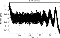
(c) Hypergamy $h,$ for 50 runs

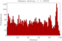
(d) Female status histogram, for one run

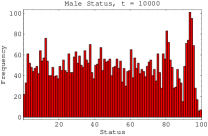
(e) Male status histogram, for one run

Figure 10: Marriage frequency, hypergamy $h,$ and status histograms at $t=10,000$ marriages, for the model $\mathbf{M}_{5}$ from Section 4.2, using the learning algorithm $\mathbf{S}_{2}.$ Children inherited the average of their parents’ statuses, and agents did not achieve any status over their lifetimes.

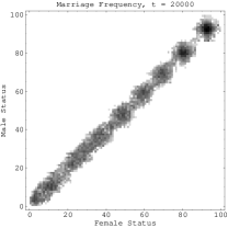
(a) Marriage frequency,
for one run

(b) Hypergamy $h,$ for one run

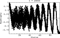
(c) Hypergamy $h,$ for 50 runs

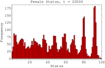
(d) Female status histogram, for one run

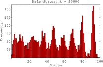
(e) Male status histogram, for one run

Figure 11: Marriage frequency, hypergamy $h,$ and status histograms at $t=20,000$ marriages, for the model $\mathbf{M}_{5}$ from Section 4.2, using the learning algorithm $\mathbf{S}_{2}.$ Children inherited the average of their parents’ statuses, and agents did not achieve any status over their lifetimes.

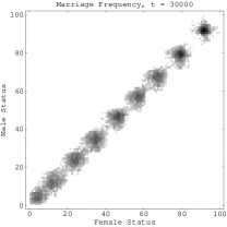
(a) Marriage frequency,
for one run

(b) Hypergamy $h,$ for one run

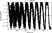
(c) Hypergamy $h,$ for 50 runs

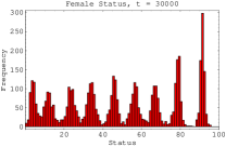
(d) Female status histogram, for one run

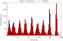
(e) Male status histogram, for one run

Figure 12: Marriage frequency, hypergamy $h,$ and status histograms at $t=30,000$ marriages, for the model $\mathbf{M}_{5}$ from Section 4.2, using the learning algorithm $\mathbf{S}_{2}.$ Children inherited the average of their parents’ statuses, and agents did not achieve any status over their lifetimes.

(a) Marriage frequency,
for one run

(b) Hypergamy $h,$ for one run

4.3 Achieved Status

In the previous models, agents inherited status at birth but did not achieve or lose any status over their lifetimes. What happens if achieved status is added? Models $\mathbf{M}_{4},\mathbf{M}_{5},$ and $\mathbf{M}_{6}$ from Section 4.2 were modified so that agents achieved or lost an amount of status $s_{\mathrm{a}}$ drawn from a Gaussian distribution with mean $\mu=0$ and standard deviation $\sigma=2.0,$ producing models $\mathbf{M}_{7},\mathbf{M}_{8},$ and $\mathbf{M}_{9}.$ An agent’s overall status was then simply the sum of its inherited and achieved statuses: $s=s_{\mathrm{i}}+s_{\mathrm{a}}.$ Just as in Section 4.2, both children inherited the average of their parents’ overall statuses, and children’s sex was determined randomly. The results at $t=100,000$ marriages are shown in Figure 18 for model $\mathbf{M}_{7}$ using the rational strategy $\mathbf{S}_{1}$ from Section 4.1.1, Figure 19 for model $\mathbf{M}_{8}$ using the learning algorithm $\mathbf{S}_{2}$ from Section 4.1.2, and Figure 20 for model $\mathbf{M}_{9}$ using the interval strategy $\mathbf{S}_{3}$ from Section 4.1.3.

As can be seen, this type of achieved status acts as a type of noise, smoothing out the status distribution and filling in the gaps caused by inheritance. Gaps still occur in the status histogram if the spread $\sigma$ of achieved status is small relative to the class size. However, the peaks do not narrow past a point determined by $\sigma,$ and if $\sigma$ is large enough, the status distribution remains smooth. Thus, this force acts in opposition to the inheritance force from Section 4.2.

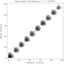
(a) Marriage frequency,
for one run

(b) Hypergamy $h,$ for one run

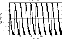
(c) Hypergamy $h,$ for 50 runs

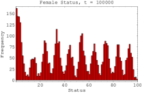
(d) Female status histogram, for one run

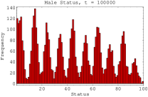
(e) Male status histogram, for one run

Figure 18: Marriage frequency, hypergamy $h,$ and status histograms at $t=100,000$ marriages, for the model $\mathbf{M}_{7}$ from Section 4.3, using the rational strategy $\mathbf{S}_{1}.$ Children inherited the average of their parents’ statuses, and agents achieved status over their lifetimes, according to a Gaussian distribution with $\mu=0$ and $\sigma=2.0$.

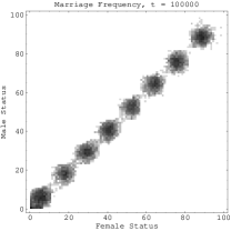
(a) Marriage frequency,
for one run

(b) Hypergamy $h,$ for one run

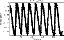
(c) Hypergamy $h,$ for 50 runs

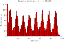
(d) Female status histogram, for one run

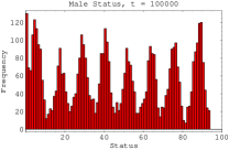
(e) Male status histogram, for one run

Figure 19: Marriage frequency, hypergamy $h,$ and status histograms at $t=100,000$ marriages, for the model $\mathbf{M}_{8}$ from Section 4.3, using the learning algorithm $\mathbf{S}_{2}.$ Children inherited the average of their parents’ statuses, and agents achieved status over their lifetimes, according to a Gaussian distribution with $\mu=0$ and $\sigma=2.0$.

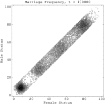
(a) Marriage frequency,
for one run

(b) Hypergamy $h,$ for one run

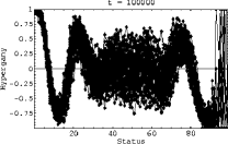
(c) Hypergamy $h,$ for 50 runs

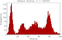
(d) Female status histogram, for one run

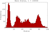
(e) Male status histogram, for one run

Figure 20: Marriage frequency, hypergamy $h,$ and status histograms at $t=100,000$ marriages, for the model $\mathbf{M}_{9}$ from Section 4.3, using the interval around self strategy $\mathbf{S}_{3}.$ Children inherited the average of their parents’ statuses, and agents achieved status over their lifetimes, according to a Gaussian distribution with $\mu=0$ and $\sigma=2.0$.

5 Conclusion

This paper has presented a variety of agent-based mathematical and computer models that can produce class endogamy, based on Marcus and Flannery’s verbal model [21]. One force that can produce class endogamy occurs if agents are only willing to marry suitors having status no less than some fixed value below the status of their highest-status suitor. This result was proved mathematically in Section 3.1 by generalizing and simplifying Burdett and Coles’s model [3, 4], and verified with a computer model in Section 4.1.1. Moreover, the simulation results in Section 4.1.2 showed that agents can easily learn the status of their highest-status suitor, reducing the amount of rationality required for class endogamy to be produced. Section 4.2 demonstrated that another such force results if children inherit the average of their parents’ statuses. This force can produce multimodality and gaps in the status distribution. If this effect is strong enough, class endogamy results simply due to a scarcity of potential mates outside of the local peak in the status histogram. In fact, actual gaps can appear in the status histogram. In contrast, Section 4.3 showed that status achieved over an agent’s lifetime can be viewed as noise, analogous to mutation in biological evolution, counteracting the inheritance force and having the effect of smoothing out the status distribution. I propose that class endogamy may have been produced by the interaction of forces such as these, along with other factors such as ideology. (This is analogous to the manner in which biological evolution is the product of multiple forces including natural selection, crossover, mutation, and genetic drift [11].) In sum, these models have shown that simple, plausible heuristic mechanisms can in theory produce class endogamy. How stupid can agents be and still form social strata? Perhaps rather stupid, indeed. Whether these models have any bearing on how class endogamy actually evolved in any particular human society must of course be tested against the ethnographic, ethnohistorical, archaeological, and psychological data.

One question raised by these models is, if these mechanisms can reliably and quickly produce class endogamy, why didn’t class endogamy and social stratification emerge immediately after ranked societies developed? In other words, why do chiefdoms exist at all in the historical and archaeological record? One possible answer is that complex chiefdoms seem to have been unstable, with recurring cycles of aggregation into complex chiefdoms followed by collapse into smaller and simpler chiefdoms [35]. Chiefdoms, without social stratification, may simply have been a more stable organizational form. (However, even chiefdoms seem to have been somewhat unstable, sometimes collapsing into unranked societies [20].) Another answer may be that newly-developed chiefdoms were relatively small and egalitarian, and became larger and less egalitarian only over time. If the status difference between the highest- and lowest-status members of a society was relatively small, and the selection of eligible mates was small as well, then individuals may have been less selective, reducing the impact of the forces described here. Finally, there was likely resistance to stratification that took time to overcome.

Burdett and Coles [3, 4] argue that their model applies to contemporary Western societies. I am dubious about applying these models to the present day. First, the models assume that men and women choose whether to marry based on a single factor: status. In contrast, there seem to be multiple factors upon which men and women base their decisions in modern societies, such as personality, common interests, intelligence, education, wealth, and physical attractiveness, as well as social status. While married couples seem to be positively correlated for many such factors [3], correlation alone does not imply endogamy, as was shown in Section 4.1.3. Furthermore, these models assume that men and women each have a single overall desirability metric for the opposite sex. However, in contemporary societies, different people often weight these factors very differently: Two men can easily disagree as to how desirable a woman is, and vice versa. In general, it is unclear whether endogamous classes form by these mechanisms in modern societies. In contrast, religions and ethnicities may form endogamous groups; however, these are relatively discrete groups to begin with, in contrast to the continuous status distributions considered here. The same is true of education, since it is usually achieved in discrete amounts and classified into categories such as “MBA from an Ivy League university”.

6 Future Work

The most obvious extension of this paper would be to test whether the mechanisms proposed here were in fact present in any real societies, using ethnographic, ethnohistorical, and archaeological data. It is also important to test whether the type of class endogamy produced by these models is consistent with that in real societies. One possible source of empirical data is the Human Relations Area Files (HRAF) [14]. It might also be possible to devise psychological tests to examine whether the rational strategy $\mathbf{S}_{1}$ from Section 4.1.1 is realistic within some particular contemporary society.

Another immediate extension to the model would be to add randomness or noise to the agents’ decision making under the various strategies, in order to test how robust the emergence of class endogamy is. This noise would represent such factors as chance events, imperfect information, and love. (In contrast, in contemporary Western societies, the effects of social status could be considered as noise in relation to the dominant effects of love and attraction.) It would also be useful to define a class endogamy metric, so that simulation results could be compared objectively. One such metric could be the average distance between local minima and maxima on the hypergamy plots, but this breaks down as a proxy for measuring class endogamy if the peaks in the status histogram are very narrow, as can be seen in Figure 9. Finally, Miller’s Active Nonlinear Tests (ANTs) [23] could be used to search for regions of parameter space where these models break down.

Another way to make the model more realistic would be to add death and reproductive rates that vary by agent age [33], and perhaps some form of discounting. Multidimensional status could be added as well, with agents weighing such factors as social status, wealth, education, and attractiveness to produce an overall status or desirability score. It seems likely that this would be an obstacle to class formation, like noise, since it would increase the likelihood for agents who would otherwise be in separate classes, based on social status alone, to marry.

More aspects of the models could be analyzed mathematically, for instance the rate of regression towards the mean when inherited status is averaged, the magnitude of the smoothing caused by achieved status, and the conditions under which the learning algorithm $\mathbf{S}_{2}$ is effective.

Henry Wright has proposed another verbal model of the evolution of class endogamy:

Neither the difficult question of why some societies ascribe the right to make community-wide decisions to office-holders drawn from a limited social sub-group, nor the question of why some networks of simple ascriptively ranked societies develop social classes are crucial to this essay. Regarding the latter question, it suffices to suggest that — if productive systems can sustain a continuity of the social network in time (and many cannot) — with time, intermarriages and disputes among the ranking families will disperse claimants to office. Many individuals may compete for offices with which few will have any local connection. Indeed, the ranking or noble class as a whole can be expected to oppose any local interests. Thus, the development within a network of chiefly polities of a class competing for positions, but opposing others outside the class, may be simply explained. [35, pp. 70–71]

It would be interesting to implement this model on a computer, to verify whether such distributed intermarriage is indeed another mechanism for producing class endogamy. Such a model would be more complicated than the ones presented in this paper, however. The set of agents eligible for the office of chief would have to be explicitly defined, as well as the effect of office holding on status, the network of chiefdoms, and the conditions under which two agents from separate chiefdoms would marry.

Another mechanism might result from the interaction between hypogamous marriage and the averaging of inherited status. As a thought experiment, consider the following situation: A paramount chief, with status $99,$ arranges a hypogamous marriage between one of his daughters, also with status $99,$ and a subchief in an outlying village, with status $49.$ The inhabitants of the paramount’s seat have status ranging from $0$ to $99,$ while those in the subchief’s village have status from $0$ to $49.$ If children inherit the average of their parents’ statuses, then the offspring of this marriage would have a status of $(99+49)/2=79$ at birth, far outranking both their father and all of the other local villagers. Such offspring would thus naturally look outside of their own village for potential mates, leading to the kind of noble class that Wright refers to. This model, while merely a caricature, demonstrates another way in which gaps in a chiefdom’s status distribution could have resulted, in addition to the inheritance force from Section 4.2.

One last extension might be to keep track of the agents’ lineages over time and examine what effect the mechanisms presented here had on their genealogical trees.

Finally, similar models have been used to study the causes of sympatric speciation [12]. It would be interesting to investigate whether there are analogies, at an abstract mathematical level, between class endogamy and biological speciation.

References

- [1] Robert Axelrod. The Complexity of Cooperation: Agent-Based Models of Competition and Collaboration. Princeton University Press, Princeton, 1997.
- [2] Robert Axelrod. Disseminating culture. In The Complexity of Cooperation: Agent-Based Models of Competition and Collaboration [1], chapter 7, pages 145–177.
- [3] Ken Burdett and Melvyn G. Coles. Marriage and class. The Quarterly Journal of Economics, 112(1):141–168, February 1997.
- [4] Ken Burdett and Melvyn G. Coles. Transplants and implants: The economics of self-improvement. International Economic Review, 42(3):597–616, August 2001.
- [5] Robert L. Carneiro. The chiefdom: Precursor of the state. In Grant D. Jones and Robert R. Kautz, editors, The Transition to Statehood in the New World, pages 37–73. Cambridge University Press, Cambridge, 1981.
- [6] Timothy K. Earle. Economic and social organization of a complex chiefdom: The Halelea district, Kauai, Hawaii. Anthropological Papers of the Museum of Anthropology 63, University of Michigan, Ann Arbor, 1978.
- [7] Joshua M. Epstein and Robert Axtell. Growing Artificial Societies: Social Science from the Bottom Up. MIT Press, Cambridge, MA, USA, 1996.
- [8] Kent V. Flannery. The cultural evolution of civilizations. Annual Review of Ecology and Systematics, 3:399–425, 1972.
- [9] Kent V. Flannery. Prehistoric social evolution. In Carol R. Ember and Melvin Ember, editors, Research Frontiers in Anthropology, pages 1–26. Prentice-Hall, Englewood Cliffs, NJ, USA, 1995.
- [10] Morton H. Fried. The Evolution of Political Society: An Essay in Political Anthropology. Random House, New York, 1967.
- [11] Douglas J. Futuyma. Evolutionary Biology. Sinauer, Sunderland, MA, USA, third edition, 1998.
-
[12]
Rainer Hilscher.
Plug and simulate: A study of the implications of individual mating
decisions on speciation dynamics using an agent based modeling approach.
Presented at SwarmFest 2004, Ann Arbor. URL
http://www.cscs.umich.edu/swarmfest04/Program/PapersSlides/HilscherSwarm2004- 040507.pdf. - [13] John H. Holland. Hidden Order: How Adaptation Builds Complexity. Addison-Wesley, Reading, MA, USA, 1995.
- [14] Human Relations Area Files (HRAF). URL http://www.yale.edu/hraf/.
- [15] Tim Ingold, David Riches, and James Woodburn, editors. Hunters and Gatherers. Berg, New York, 1988.
- [16] Patrick Vinton Kirch. The Evolution of the Polynesian Chiefdoms. Cambridge University Press, Cambridge, 1984.
- [17] Timothy A. Kohler and George J. Gumerman, editors. Dynamics in Human and Primate Societies: Agent-Based Modeling of Social and Spatial Processes. Oxford University Press, New York, 1999.
- [18] Timothy A. Kohler, James Kresl, Carla Van West, Eric Carr, and Richard H. Wilshusen. Be there then: A modeling approach to settlement determinants and spatial efficiency among late ancestral Pueblo populations of the Mesa Verde region, U.S. Southwest. In Kohler and Gumerman [17], pages 145–178.
- [19] J. Stephen Lansing. Anti-chaos, common property, and the emergence of cooperation. In Kohler and Gumerman [17], pages 207–223.
- [20] Edmund R. Leach. Political Systems of Highland Burma: A Study of Kachin Social Structure. Harvard University Press, Cambridge, MA, USA, 1954.
- [21] Joyce Marcus and Kent V. Flannery. Zapotec Civilization: How Urban Society Evolved in Mexico’s Oaxaca Valley. Thames and Hudson, London, 1996.
- [22] William H. McNeill. Plagues and Peoples. Anchor, New York, 1976.
-
[23]
John H. Miller.
Active nonlinear tests (ANTs) of complex simulation models.
SFI Working Paper 96-03-011, Santa Fe Institute, Santa Fe, NM, USA,
1996.
URL http://www.santafe.edu/sfi/publications/Working-Papers/96-03-011.ps. - [24] Colin Renfrew. Archaeology & Language: The Puzzle of Indo-European Origins. Cambridge University Press, Cambridge, 1987.
- [25] Mitchel Resnick. Turtles, Termites, and Traffic Jams: Exploration in Massively Parallel Microworlds. MIT Press, Cambridge, MA, USA, 1994.
- [26] Robert G. Reynolds. An adaptive computer model for the evolution of plant collecting and early agriculture in the eastern valley of Oaxaca. In Kent V. Flannery, editor, Guilá Naquitz: Archaic Foraging and Early Agriculture in Oaxaca, Mexico, chapter 31, pages 439–500. Academic Press, Orlando, FL, USA, 1986.
- [27] Marshall D. Sahlins. Poor man, rich man, big man, chief: Political types in Melanesia and Polynesia. Comparative Studies in Society and History, V:285–303, 1963.
- [28] Thomas C. Schelling. Micromotives and Macrobehavior. Norton, New York, 1978.
- [29] Elman R. Service. Primitive Social Organization: An Evolutionary Perspective. Random House, New York, 1962.
- [30] Elman R. Service. Origins of the State and Civilization: The Process of Cultural Evolution. W. W. Norton, New York, 1975.
- [31] Julian H. Steward. Theory of Culture Change: The Methodology of Multilinear Evolution. University of Illinois Press, Urbana, 1955.
- [32] Gérard Weisbuch, Guillaume Deffuant, Frédéric Amblard, and Jean-Pierre Nadal. Meet, discuss, and segregate! Complexity, 7(3):55–63, 2002.
- [33] Kenneth M. Weiss. Model life tables for anthropology. Memoirs of the Society for American Archaeology, 27, 1973.
- [34] Henry T. Wright. Recent research on the origin of the state. Annual Review of Anthropology, 6:379–397, 1977.
- [35] Henry T. Wright. Prestate political formations. In Gil Stein and Mitchell S. Rothman, editors, Chiefdoms and Early States in the Near East: The Organizational Dynamics of Complexity, volume 18 of Monographs in World Archaeology, pages 67–84. Prehistory Press, Madison, WI, USA, 1994.