Logarithmic periodicities in the bifurcations of type-I intermittent chaos

Abstract

The critical relations for statistical properties on saddle-node bifurcations are shown to display undulating fine structure, in addition to their known smooth dependence on the control parameter. A piecewise linear map with the type-I intermittency is studied and a log-periodic dependence is numerically obtained for the average time between laminar events, the Lyapunov exponent and attractor moments. The origin of the oscillations is built in the natural probabilistic measure of the map and can be traced back to the existence of logarithmically distributed discrete values of the control parameter giving Markov partition. Reinjection and noise effect dependences are discussed and indications are given on how the oscillations are potentially applicable to complement predictions made with the usual critical exponents, taken from data in critical phenomena.

Dynamical bifurcations, when the qualitative behavior of a natural phenomena changes due to the variation of a control parameter, is a subject described by a well founded mathematical theory Crawford (1991). Their extension from equilibrium thermodinamic phase transitions to the bifurcations in non-equilibrium systems is applied within and outside physics Manneville (1990); Sornette (1998). Some bifurcations are abrupt, like first order equilibrium transitions, and others follow critical relations with a continuous dependence in the control parameter. Sufficiently close to the bifurcation the system properties follow characteristic functions giving rise to critical exponents which are signatures of the phenomena. Log-periodic oscillations modulating critical functional relations have been reported in studies of bifurcations Sornette (1998); Gluzman and Sornette (2002). As reviewed by Sornette Sornette (1998), many ongoing research on applications are active, among them the prediction of catastrophic events. Transient chaos Grebogi et al. (1983) and other escape phenomena Maier and Stein (1996) also display such log-periodicities. In simple maps, the period doubling Feigenbaum cascade is an early example where log-periodic behavior appears Derrida (1978). In non attracting sets of two dimensional maps, the topological entropy have been shown to present log-periodic oscillations Vollmer and Breymann (1994).

Among the dynamical bifurcation phenomena many can be cast on the class of intermittent chaos, ranging from the onset of turbulence Bergé et al. (1980) to synchronism of chaotic systems Zhan et al. (2001); Rosenblum et al. (1996). As originally proposed by Pomeau and Manneville Pomeau and Manneville (1980); Bergé et al. (1980); Manneville (1990), these instabilities can be modeled with simple one-dimensional maps and classified as type-I, II, and III, according to the Floquet multipliers of the map crossing the unity circle in the complex plane at $1$, at a pair complex conjugate values or at $-1$, respectively. Type I, which will be discussed here, occurs when a saddle-node or tangent bifurcation is approached. Iterations of the map near the value of the virtual fixed points are identified with the laminar events while the reinjection iterates correspond to the turbulent bursts that occur in a erratic manner. Such bifurcation has been reported in many experimental systems Jeffries and Perez (1982); Lefranc et al. (1991) and it is abundant in the logistic and other simple maps. Renormalization group procedure to deal with type-I intermittency has already been used Hirsch et al. (1982) and give analytical asymptotic expressions for statistical averages in the maps. These are treatments that only give smooth critical dependences.

The tangent bifurcation has analogy with second order thermodynamic phase transitions. The continuous scale invariance of thermodynamical phase transitions gives smooth monotonic critical relations for the statistical thermodynamical variables or the susceptibilities, as the order parameter approaches the transition. However, as mentioned above, oscillations do occur in the corresponding properties of non-equilibrium dynamical bifurcations. Discrete scale invariance in the dynamical systems bifurcations underly the oscillating features Sornette (1998). In type-I intermittent chaos with the tangency having second and fourth order nonlinearity, they appear with power-law periodicity de S. Cavalcante et al. (2001); de S. Cavalcante and Rios Leite (2004), instead of log-periodicity.

Herein, to study the origin and properties of the log-periodic undulations, the simplest unidimensional map exhibiting chaos and a saddle-node bifurcation was considered. It is a piecewise linear map first proposed to study critical scaling laws of type-I intermittency by Shobu et al. (1984). A reason to take this map is the existence of an analytical approach to find the discrete values of the control parameter at which the scaled shape of the map function reproduces itself. The average length of laminar phases, the spectrum of fractal dimensions, the Lyapunov exponent, and the statistical moments of the chaotic variable, when calculated numerically, show log-periodic oscillation. Such numerical results correspond to time averages and became possible due to the great computational power achieved with current digital machines. They can be compared to, and surpass in detail, analytical results from averages in ensembles valid at specific values of the control parameter. The oscillation reported here are one such case. Unfortunately we were unable to extend the theory of renormalization group Hirsch et al. (1982) to predict such periodic property.

The equation for the map is Shobu et al. (1984)

$$x_{n+1}=\left\{\begin{array}[]{ll}ax_{n}+b,&\mathrm{for}\ x_{n}\leq c\\ a^{-1}[x_{n}-(1-b)]+1,&\mathrm{for}\ c<x_{n}\leq 1-b\\ -b^{-1}(x_{n}-1),&\mathrm{for}\ x_{n}>1-b\end{array}\right.$$ (1)

where $0<b<1/2$ is a constant , $a=1-2b+\epsilon>0$, and $c=(1-b)/(1+a)>0$ are expressed as functions of the control parameter $\epsilon$. The map is represented in figure 1 with $b=0.2$ and $\epsilon=0.0332$.

Figure 1: The So-Ose-Mori map with an unstable periodic orbit, calculated with $b=0.2$ and $\epsilon=0.0332$.

When $\epsilon<0$ the first two linear segments cross the diagonal and a stable fixed point exists at the first crossing. At $\epsilon=0$ the corner point of the first two linear segments touch the diagonal, at $x=1/2$, and a bifurcation occurs similar to a saddle-node when two fixed points disappear. For $\epsilon>0$, only the third linear segment intersects the diagonal with an absolute value of slope greater than 1 and the map is chaotic. Iterates at left of $(1-b)$ shall be considered as laminar, and iterates on the negative slope will be referred to as reinjection events. With $\epsilon>0$, $c$ is approximately proportional to the minimum distance between the map and the $y=x$ diagonal.

Shobu et al. (1984) have shown that, for this map, simple Markov partitions exist at discrete values of $\epsilon$. When this happens, as one iterates the map, the probability of visits, or the natural measure, over the unit interval is a countable set of step intervals with constant value. The map dynamics is that of a finite Markov chain, diverging for $\epsilon\rightarrow 0$, and it is analytically solvable. The appearance of unstable periodic orbits, reinjecting at $x=0$ and iterating $2n+2$ times until reaching precisely the value $1$, mark the condition for the Markov partition with $2n+1$ constant steps for the natural measure. Figure 1 shows the map and the iterates of such an orbit with period 12. The specific values of $\epsilon=\epsilon_{n}$ for which the orbit of period $2n+2$ exists follow the recursive relation $\epsilon_{n}=(1-2b)\epsilon_{n-1}$ Shobu et al. (1984), and, as good approximation for $n>3$,

$$\epsilon_{n}=2b\left(\frac{1-b}{1+b}\right)(1-2b)^{n-1}.$$ (2)

The factor $(1-2b)$ will appear as the period of the fine structure in logarithmic scale. At the values of $\epsilon_{n}$ one can obtain analytically the ensemble averages for the average length of laminar events, $\left<l\right>$, for the first order moment of the attractor, $\left<x\right>$, Shobu et al. (1984), and for the Lyapunov exponent, $\left<\lambda\right>$, The analytical expressions first determined by Shobu et al. (1984), and resulting from the summation with the stepwise uniform probabilistic measure, are

$$\left<l\right>\cong\frac{1}{\ln(1-2b)}\ln\left(\frac{1}{\epsilon_{n}}\right)\ ,$$ (3)

$$\left<x\right>\cong\frac{1}{2}+\frac{1}{2n}\ ,$$ (4)

and

$$\left<\lambda\right>\cong\frac{1}{n}\left[\ln\frac{1}{b}+\frac{1}{(b-2)}\ln\frac{1}{(1-2b)}\right].$$ (5)

The ensemble averages must coincide with time averages $\overline{l}$, $\overline{\lambda}$ and $\overline{x}$, calculated using iterations of the map and starting from typical initial conditions. The length of a laminar event is considered as the number of iterations “in the channel” before a reinjection. Any consideration of a narrower range around the corner point as the channel causes just a shift in the value of $\overline{l}$ for a given $\epsilon$, but the slope and fine structure dependence on $\epsilon$ remains the same. The Lyapunov exponent (we use $\lambda$ for $\overline{\lambda}$ and$\left<\lambda\right>$) was calculated numerically using a large number of iterations, $N$, with the expression

$$\lambda=\frac{1}{N}\sum_{n=1}^{N}\ln\left|f^{\prime}(x_{n})\right|,$$ (6)

and the average of the dynamical variable $\overline{x}$ with

$$\overline{x}=\frac{1}{N}\sum_{n=1}^{N}x_{n}.$$ (7)

Figure 2 shows the average length of laminar events calculated both with time averages and ensemble average. In the last case, only a discrete set of values of $\epsilon$ from eq. 2 can be done. The values of $\overline{l}$ decrease with the control parameter $\epsilon$. Thus if one calculates and interpolates the analytical discrete values Shobu et al. (1984) one never gets the periodic effects. Conversely, for the time averages the values of $\epsilon$ can be picked at will.

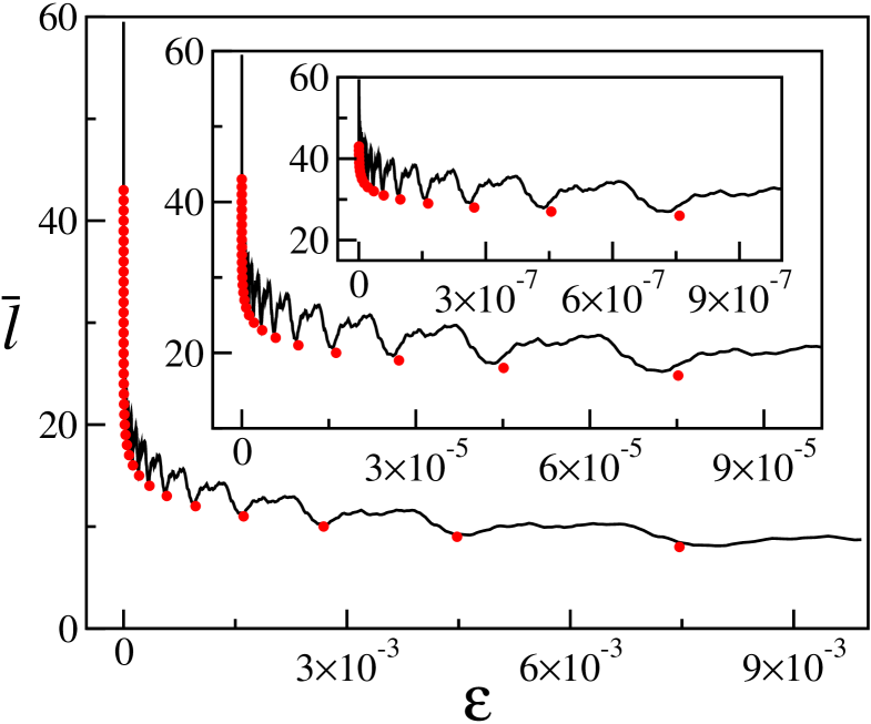
Figure 2: Average length of laminar events. The dots are analytical ensemble averages and the continuous curves are numerical time averages, iterating the map, as discussed in text.

In the figure for $\overline{l}$, 2000 values of the control parameter $\epsilon$ were equally spaced on a logarithmic scale and at each one, $N=3\times 10^{7}$ iterations were done for the averages, with double precision floating point arithmetics. One observes clearly that, in addition to the smooth power-law divergence as $\ln\epsilon^{-1}$, $\overline{l}$ is decorated with a modulation whose period is given by the positions at which each Markov partition is formed.

Numerical computations of the average length of laminar events and average Lyapunov exponent are show in fig. 3. Logarithmic scale is used in the absciss and the critical behavior of $\overline{l}$ has a linear smooth envelope behavior as $\ln\epsilon^{-1}$ for small $\epsilon$.

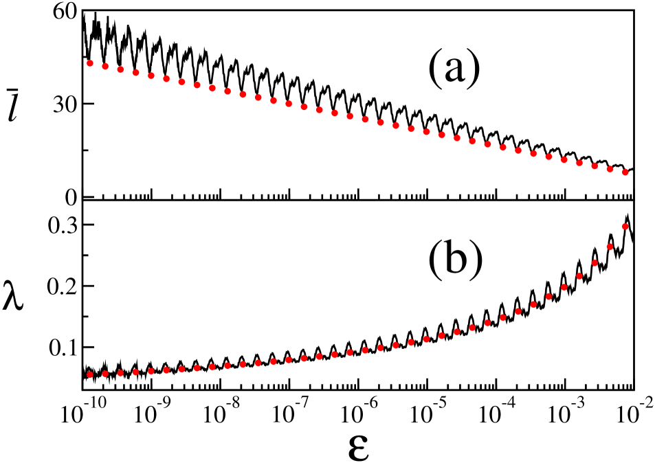
Figure 3: Average length of laminar events (a), and (b) average Lyapunov exponent, $\lambda$, in the SOM map. The dots are analytical ensemble averages and the continuous curves are numerical time averages.

Furthermore, its oscillations are periodic as function of $\ln\epsilon$. The behavior for $\left<x\right>$ is proportional to the one exhibited by $\lambda$, as one expects comparing eqs. 4 and 5. Changing $b$ on equation 1 changes the spacing between successive $\epsilon_{n}$, and the corresponding period obtained in time averages follows consistently with the scaling factor $\epsilon_{n}/\epsilon_{n+1}=(1-2b)$. Therefore, numerical artifacts for log-periodicity are completely ruled out in the computations. This $b$ dependency is shown in fig. 4. The same oscillating features were obtained (not show here) for $D_{q}(\epsilon)$, the fractal dimension of the attractor, calculated for $q=0,1$ and $2$.

Figure 4: Average of the dynamical variable in the SOM map with different scaling factor: (a) $b=0.2$ and (b) $b=0.3$.

The critical exponent of the smooth envelope of any of the averages do not change with $b$.

Calculations were also done using a random reinjection value in a map with the two first linear segments as the laminar phase part of eq. 1. As long as the reinjection is non singular, oscillations with the same period are always obtained. This fact is indication of the local nature of the oscillations. While the Markov partitions of the SOM maps are a global result, their relevant contributions for statistical averages near criticality come from the uniform density steps near the narrow channel. Any approximately uniform reinjection on this region suffices to give oscillating averages.

Finally some discussion on noise. The effects of noise in type-I intermittency have been studied analytically Hirsch et al. (1982) and experimentally Cho et al. (2002). Here, a term of additive gaussian white noise with amplitude $D$ was added to the right hand side of eq. 1. Fig. 5 shows $\overline{l}$, when the noise amplitude was $D=10^{-6}$.

Figure 5: Averages length of laminar events in the SOM map with additive noise.

For $\epsilon\gg D$ one expects the dynamics to remain unaffected. When the separation between successive $\epsilon_{n}$ becomes of the order of the noise amplitude, $D$, the corresponding and smaller oscillations are blurred out. For even smaller $\epsilon$ ($\lesssim D$), the number of iterations in the narrowest part of the channel no longer depends on $\epsilon$, because a single noise event may cause a jump across the waist of the channel, which, otherwise would have a number of iteration proportional to $\ln\epsilon^{-1}$. Therefore, $\overline{l}$ saturates. Such noise sensitivity is shown for $\overline{x}$ in fig. 6. It is relevant to observe that, consistent with the above explanation, in both figures, 5 and 6, the oscillations cease to exist for $\epsilon$ one order of magnitude higher than the value at which the slope of the average saturates. One also may see a smoothing of the ultrafine structures on the undulations. Smoothing, erasure of the undulations, and saturation of the amplitude envelope also occurs in the Lyapunov exponent when noise is present.

Figure 6: Average of the dynamical variable, $\overline{x}$, in the SOM map with additive noise.

It may also be observed in the figures that the amplitude of the undulations on $\overline{l}$ and $\overline{x}$ are bigger at different ranges of $\epsilon$. This might be used to justify the importance of acquisition of different data series and different averaged quantities in experiments.

To conclude it must be stressed that oscillations in the critical behavior of statistical properties occur universally in the tangent bifurcations of unidimensional normal form maps de S. Cavalcante and Rios Leite (2004) and in the logistic map de S. Cavalcante et al. (2001). They also occur in the saddle-node bifurcations of continuous chaotic systems, as we verified numerically integrating the Rössler, the Lorenz and the equations for a laser with saturable absorber de S. Cavalcante and Rios Leite (2000). However none of these follow the log-periodic dependence. The map herein was chosen to stress the relationship between log-periodic fine structures, existence of Markov partition and self similar scalling. From a mathematical point of view much more remains to be done on this connection. The undulations are important features of bifurcations that can be subject to experimental tests and applications. To the present, in experiments with intermittent chaos only the smooth critical behavior have been studied. The observation of log-periodic oscillations has been proposed as a technique to anticipate the criticality in natural phenomena, particularly in earthquakes Sornette (1998). The simple map presented here is far from modeling earthquakes but it is an workable example to show how the critical value of a parameter controlling bifurcations might be predicted ahead of criticality, by complementary fitting of oscillations in the fine structure at higher values of the control parameter, along with the usual fitting of the monotonic critical behavior. It also shows how improvement in extracting information on a bifurcation with intermittent chaotic should be enhanced by measuring different statistical variables on different ranges of the control parameter.