Coupled Chaotic Oscillators and Its Relation with Artificial Quadrupeds’ Central Pattern Generator

Abstract

Animal locomotion employs different periodic patterns known as animal gaits. In 1993 Collins and Stewart achieved the characterization in quadrupeds and bipeds by using permutation symmetries groups which impose constrains in the locomotion centre called Central Generator Pattern (CGP) in the animal brain. They modelled the CGP by coupling four non linear oscillators and with the only change in the coupling it is possible to reproduce all the gaits. In this work we propose to use coupled chaotic oscillators synchronized with the Pyragas method not only to characterize the CGP symmetries but also evaluate the time serie behaviour when the foot is in contact with the ground for futures robotic applications.

I Introduction

Lately the analysis of animal gaits have regain interest in between scientist of different areas. The moderm analysis represents the gait as cyclic patterns in the movements of symmetrically placed limbs. A cycle means the interval between successive footstrikes of the same foot during the dynamical process. The factor of footstrike $\beta$ is the fraction of cycle when the foot is in contact with the surface. For simplicity we assume $\beta$ to be the same for all animal feet. The relative phase of foot ($\phi$) is defined as the fraction of cycle between the contact of the surface of the foot of reference and another foot when this one enters in contact with surfaceGray (1968). In this study the relative phase plays a crucial role to formulate the symmetries while this is not same the factor of footstrike $\beta$, which will no be taken into account in this work. The mammal phenotypes have evolved in two kind of gaits, bipedal gaits where the limbs can be out of phase (walking or running) or in phase (jumping or hopping). Quadrupedal gaits with a more complex behaviour of the realtive phase. The natural gaits areAlexander (1984): Walk, the limbs move with a quarter of cycle out of phase, where there is a quarter cycle phase difference in between both fore limbs as well as in between hind lims, and half a cycle between diagonals. Trot, the diagonal legs move in phase and this pair is half a cycle out of phase of the other one. Pace or Rack, the fore and hind left or roght limbs are paired and moved half cycle out of phase in between the pairs. Canter, the right front leg and the left hind leg move in phase, the left front leg and the right hind leg move half a cycle out of phase in between themselves and out of phase with respect to the first pair (it was found in horse that pattern changes from walk to trot, to canter to gallop, when the speed increase). Bound, the fore legs move in phase, as well as the hind legs, while they move half a cycle out of pahse. Transverse Gallop, the front and hind left (right) legs move one quarter of cycle out of phase, the front (hind) limbs are slightly out of phase between themselves. Rotatory Gallop, similar to the tranverse gallop but the left and right limbs have their pattern exchange. Pronk, the four limbs move together an in phase.

Biological model assume that the animal nrevous system contains a variety of Central Pattern GeneratorsA. Cohen and Grillner (1988) (CPG), each oriented to specific action. For instance, the locomotion CPG controls the rhythm of mammal gaitDagg (1973), in the case of quadrupedal mammals this is modeled by a system of coupled cell where erach cell is composed by a set of neurons directly responsible to harmonize the movement of the legGlass and Young (1979). A simplifield mathematical model of locomotion CPG consists in replacing each cell by a non linear oscilatorCollins and Stewart (1993). This model has been studied using differnt method: bifurcation theory, numerical simulations and phase reponseAlexander and Goldspink (1977); Hildebrand (1964); Hildelbrand (1965); Collins and Richarmond (1994).

The idea to study rhythmic patterns in animal gait using symmetries models was introduced by HildebrandHildelbrand (1965), Schoner et alC. Canvier and Byrne (1997). The concept of symmetries in coupled cells as a model for locomotion CPG in quadrupedal mammals was firt used by Collins and StewartCollins and Stewart (1993). A model for locomotion CPG for quadrupedal mammals consits in a ring of four coupled nonlinear oscillators. Each oscillator represents a limb of the animal. The stability and breakdown of the symmetries play an effective role in the validity of the model. Golubitsky et alGolubistsky and Luciano (2001). argued that symmetries present in above model for walk, trot and pace are not adequade for quadrupeds, sience the trot and pace correspnd to conjugate solutions which have same stability and they depend on initial conditions. Many quadrupeds move with pace but do not trot (camels) or viceversa (horse), unless they are trained. In this work we propose a different coupling mechanism in order to avoid the problem of multiple conjugated solutionsCollins and Stewart (1993).

The CPG is modeled by the following system of ordinary differential equations:

$$\frac{dX_{j}}{dt}=f(X_{j})+h_{j}(X_{j-1},\,X_{j+1})$$ (1)

where $j=1\ldots 4$ mod 4 is the index of cell, $X\in\mathbb{R}^{n}$ is the state vector and $f:\mathbb{R}^{n}\to\mathbb{R}^{n}$ is a nonlinear velocity vector field. We defined the symmetry of ring to the permutations of cell that preserves the coupling, that is to say a permutation $\sigma$ of $\{1\ldots 4\}$ numbers on the phase space $X=(X_{1},X_{2},X_{3},X_{4})$ is:

$$\sigma X=(X_{\sigma^{-1}(1)},X_{\sigma^{-1}(2)},X_{\sigma^{-1}(3)},X_{\sigma^{-1}(4)})$$ (2)

then $\sigma$ is a symetry of ring in

$$F(\sigma X)=\sigma F(X).$$ (3)

where $F(.)=f(.)+h(.)$. Then we deduced the coupling conditions they are:

$$h_{j}(\sigma X_{j-1},\sigma X_{j+1})=h_{\sigma(j)}(X_{j-1},X_{j+1}).$$ (4)

If we defined $[i,j]$ as the action to exchange $X_{i}$ for $X_{j}$ the symmetries of the ring are: { [1,4]; [2,3]; [1,2]; [4,2] }. From eq-4 we deduced $h_{1}(.)=h_{3}(.)$ and $h_{2}(.)=h_{4}(.)$. These symmetries are called Type-2 by Collins and StewartCollins and Stewart (1993). Another kind of symetry is called symmetry of phase changeGolubistsky and Luciano (2001). Assuming that $X(t)$ is a periodic solution with minimal period (cycle) T, and $\gamma$ represents the symmetry $(ij)$ to permute $X_{i}$ for $X_{j}$, then $\gamma\,X(t)$ will be a periodic solution if the trajectories $\{X(t)\}_{t}$ and $\{\gamma X(t)\}_{t}$ coincide. Therefore the only solution is the existence of pahse slip $\theta$ such that $\gamma X_{j}(t)=X_{j}(t+\theta)$. The pair $(\gamma,\theta)$ is a spatio-temporal symmetry where $\theta$ is a phase slip. Finally we define as primary gaitGolubistsky and Luciano (2001), those gaits modeled by identical output signal of each cell but out of phase.

We associated the index of cell to each limb as follow, $j=1$ hind left, $j=2$ fore left, $j=3$ fore right and $j=4$ hind right. The possible symmetries of the primary gait for four legged animals characterized by Type-2 arrays are:

Table 1: Simmetries asocied with gait

Gait	Symmetry	Group
Stopped	$(I,\theta)$ $(\alpha,\theta)$ $(\beta,\theta)$ $(\alpha\beta,\theta)$	$D_{2}\times S^{1}$
Pronk	$(I,0)$ $(\alpha,0)$ $(\beta,0)$ $(\alpha\beta,0)$	$D_{2}$
Pace	$(I,0)$ $(\alpha,\frac{1}{2})$ $(\beta,\frac{1}{2})$ $(\alpha\beta,0)$	$\tilde{D}_{2}^{D}$
Bound	$(I,0)$ $(\alpha,0)$ $(\beta,\frac{1}{2})$ $(\alpha\beta,\frac{1}{2})$	$\tilde{D}_{2}^{F}$
Trote	$(I,0)$ $(\alpha,\frac{1}{2})$ $(\beta,0)$ $(\alpha\beta,\frac{1}{2})$	$\tilde{D}_{2}^{L}$
Rotatory Gallop	$(I,0)$ $(\beta,\frac{1}{2})$	$\tilde{Z}_{2}^{L}$
Transverse Gallop	$(I,0)$ $(\alpha\beta,\frac{1}{2})$	$\tilde{Z}_{2}^{F}$
Canter	$(I,0)$	$\mathbb{I}$

Table 1: Where $\alpha=(12)(34)$, $\beta=(13)(24)$, $\alpha\beta=(14)(23)$ and $S^{1}$ refers to all cyclic group of pahse slip mod 1. $D$ represents the diedral subgroup and $Z$ all the cyclic subgroups. The tilde indicates the existence of phase slip symmetry. The notation $\frac{1}{2}$ represents a half cycle out of phase.

Here we study the possibility to use a ring of coupled chaotic oscillators to produce the locomotion of quadrupeds based on the symmetries of primary gaits using Pyragas control theory.

II A CPG Model

Here we represented each cell by Rösler oscillators (see eq.-5) coupled using PyragasPyragas (1992) method with random initial cnditions. We use Rossler chaotic oscillator since this is the only one that have shown to synchronize to simulate the primary gait. This behaviour does not happen for Van der PoolCollins and Stewart (1993) or ShowalterV. Petrov and Showalter (1992) oscilators even if the single oscillator reproduce the necessary output. Primary gate is important for any digital aplication on mechanical limb.

$$\left\{\begin{array}[]{rcl}\frac{dx}{dt}&=&-(y+x)\\ \frac{dy}{dt}&=&x+0.2\,y\\ \frac{dz}{dt}&=&0.2\,+\,z\,(x-c)\end{array}\right.$$ (5)

We use a direct synchronization mechanism where the master variable is “$y$” and other one are the slave varibles. We use a delay time serie for obtain delay feedback value. Then coupling functions are:

$$\begin{array}[]{ll}h_{i}(X_{i},X_{i+1},X_{i-1})=k_{i}\,(y_{i-1}(t-\tau)-y_{i}(t))&\\ +g_{i}\,(y_{i+1}(t-\tau)-y_{i}(t))&\end{array}$$ (6)

The symmetry conditions associated to a Type-2 array limits the range of $k_{i}$ and $g_{i}$ values. In this case $g_{1}=k_{2}$, $g_{2}=k_{3}$, $g_{3}=k_{4}$, $g_{4}=k_{1}$, $k_{1}=k_{2}$ and $k_{4}=k_{3}$. An esquematic form it is depected in figure-1. The delay time $\tau\in\mathbb{N}$, and the nonlinear constan $c$ (see eq.-5) play an important role in the wave pattern obtained. We consider as output of each cell (oscilator) the value of the variable $x_{i}(t)$, where it will be compouse by threshold function:

$$Q(x)=\left\{\begin{array}[]{ll}0&\textrm{si $x>2.0$}\\ 1&\textrm{si $x\leq 2.0$}\end{array}\right.$$ (7)

This defined a mapping from phase space into binary matrix space of 2x2. We associate the value “1” to the state “limb on ground” and the value “0” to the state “limb in movement”, not on the ground. Finally the matrix representation is from now on:

$$\mathbf{C}=\left(\begin{array}[]{cc}\textrm{Fore Left}&\textrm{Fore Right}\\ \textrm{Hind Left}&\textrm{Hind Right}\end{array}\right)$$

Therefore the gait is nothing but the sequence of matrices of succesive states representing the symmetry of CPG. For instance the pronk is give by the sequence of matrices:

$$\left\{\left(\begin{array}[]{cc}1&1\\ 1&1\end{array}\right)\,;\,\left(\begin{array}[]{cc}0&0\\ 0&0\end{array}\right)\right\}$$

This allows a clearer visualization of the symmetries of primary gait. Although we lose the time interval between different patterns. This is highly important for application in robotics, not only it conditions actuator answers, also for the fact that mechanical inner may introduce undesirable instabilities. This is the reason that we have to analyse the time each pattern stays in periodic sequence.

We consider two type of ad hoc combinations for the coupling constants, which are the most represntatives in between the values tried. We call SA model when $k_{1}=k_{3}=0.1$ and $k_{2}=k_{4}=0.001$, SB a $k_{1}=k_{3}=0.1$ and $k_{2}=k_{4}=-0.001$. Those values were selected under the assumption of strong coordination between the limbs associated to each cerebral hemisphere, while they are weakly correlated when they belong to different hemisphere.

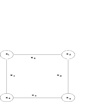
Figure 1: Cell coupling diagram.

III Numerical Results

There is a dependence of the output, on the time delay $\tau$, which is quiet robust under variations of the parameter $c$ (see eq-5 ), and it is independent of the model used, SA or SB. There is a change of state as a function of the time delay, which follow the order Chaos $\to$ Periodic Oscillations $\to$ Stable Fixed Point $\to$ Primary Hopf Bifurcation $\to$ Secondary Hopf Bifurcations $to$ Chaos when $\tau$ increases from zero. This can seen in Fig-2, where we plot the maximum Lyapunov exponet of the systems versus $\tau$. Since it is necessary to have a stable time interval in between patterns, we restrict ourselves to the interval $6\leq\tau\leq 38$.

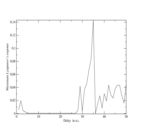
Figure 2: Maximum Lyapunov exponent verus delay.

III.1 SA Coupling

For $6\leq\tau\leq 13$, the periodic gait obtained is:

$$\left\{\left(\begin{array}[]{cc}1&1\\ 1&1\end{array}\right)\,;\,\left(\begin{array}[]{cc}0&0\\ 0&0\end{array}\right)\right\}$$

which corresponds to the pronk and the symmetry is $D_{2}$. On the other hand for $\tau=14$ the limit cycle is not stable any longer ant it appears an asymptotic stationary state, which produces the single sequence correspond to the symmetry $D_{2}\times S^{1}$, therefore a stop, since all limbs are on ground. For $\tau=34$, the fixed point loses its stability and it becomes unstable, where the orbits converge to a single limit cycle. The pattern found for the delay $34\leq\tau\leq 38$ is :

$$\left\{\left(\begin{array}[]{cc}0&1\\ 1&0\end{array}\right)\,;\,\left(\begin{array}[]{cc}1&1\\ 1&1\end{array}\right)\,;\,\left(\begin{array}[]{cc}1&0\\ 0&1\end{array}\right)\,;\,\left(\begin{array}[]{cc}1&1\\ 1&1\end{array}\right)\right\}$$

This has a symmetry $\tilde{D}_{2}^{L}$, which corresponds to the gait trot. In this case each step involves the movement of all the limbs, gait which is only observed in havy quadruopeds, above 1 ton, such as girafes and buffalosCollins and Stewart (1993). We could not find any other patterns in this interval of time delay.

III.2 SB Coupling

For $6\leq\tau\leq 13$ the coupled chaotic system oscillate in a stable limit cycle, which in this case produce the patterns:

$$\left\{\left(\begin{array}[]{cc}1&1\\ 0&0\end{array}\right)\,;\,\left(\begin{array}[]{cc}1&1\\ 1&1\end{array}\right)\,;\,\left(\begin{array}[]{cc}0&0\\ 1&1\end{array}\right)\,;\,\left(\begin{array}[]{cc}1&1\\ 1&1\end{array}\right)\right\}$$

which has symmetry $\tilde{D}_{2}^{F}$ and corresponds to a gait bound. We should mention that the true bound as the one observed in siberian squirrelCollins and Stewart (1993) implies the state of all limbs on air. On the other hand in this case all four limbs are on the ground in order to generate another step which does not exist in nature. This drawback, we resolve applying “not” operator each matrix. As in the SA case, for $14\leq\tau\leq 32$ the coupled system has stable fixed point and the limit cycle becomes unstable, which correspond to stop. For $\tau=33$ the fix point become unstable and a stable cycle appears producing the patterns:

$$\left\{\left(\begin{array}[]{cc}1&1\\ 1&1\end{array}\right)\,;\,\left(\begin{array}[]{cc}1&0\\ 1&0\end{array}\right)\,;\,\left(\begin{array}[]{cc}1&1\\ 1&1\end{array}\right)\,;\,\left(\begin{array}[]{cc}0&1\\ 0&1\end{array}\right)\right\}$$

which corresponds to gait pace with symmetry $\tilde{D}_{2}^{D}$. As describes above the horse never sets all four limbs on the ground, then applying “not” operator each matrix, we have resolved it. For this coupling the gait is not structurally stable for all time delay values. From $\tau=34$ until 4 $\tau=37$ the gait changes to another periodic pattern:

$$\left\{\left(\begin{array}[]{cc}0&1\\ 1&1\end{array}\right)\,;\,\left(\begin{array}[]{cc}1&1\\ 1&0\end{array}\right)\,;\,\left(\begin{array}[]{cc}1&0\\ 1&0\end{array}\right)\,;\,\right.$$

$$\left.\left(\begin{array}[]{cc}1&0\\ 1&1\end{array}\right)\,;\,\left(\begin{array}[]{cc}1&1\\ 0&1\end{array}\right)\,;\,\left(\begin{array}[]{cc}0&1\\ 0&1\end{array}\right)\right\}$$

With symmetry $\{(I,0)\,(\alpha,\frac{2}{3})\,(\beta,\frac{2}{3})\}$. This symmetry does not correspond to any primary gait observed in nature. For $\tau=38$ the system generates again a gaite like pace.

IV Conclusions

Pyraga’s direct synchronization (see eq 6) is a novel coupling mechanism between cell for Type-2 networks when it is used as CPG model. Within this we can avoid the conjugate undesirable solutions. But no natural patterns appear in SB model. Also we can not look for canter and transverse gallop gaits. This network type is not adequately for a natural GCP model. However it is useful as an artificial CPG mechanism in robotic science.

V References

References

- Gray (1968) J. Gray, Animal Locomotion (Weidenfeld and Nicolson, 1968).
- Alexander (1984) R. Alexander, Int. J. Robot Res. 3, 49 (1984).
- A. Cohen and Grillner (1988) S. R. A. Cohen and S. Grillner, Neural Control of Rhythmic Movements in Vertebrates (Wiley New York, 1988).
- Dagg (1973) A. Dagg, Mammal Rev. 3, 135 (1973).
- Glass and Young (1979) L. Glass and R. Young, Brain Res. 179, 207 (1979).
- Collins and Stewart (1993) J. Collins and I. Stewart, J. Nonlin. Sci. 3, 345 (1993).
- Alexander and Goldspink (1977) R. Alexander and J. Goldspink, Mechanics and Energetics of Animal Locomotion (Chapman and Hall, 1977).
- Hildebrand (1964) M. Hildebrand, Folia Biotheoretica 4, 10 (1964).
- Hildelbrand (1965) M. Hildelbrand, Science 150, 701 (1965).
- Collins and Richarmond (1994) J. Collins and S. Richarmond, Biol. Cybern. 71, 375 (1994).
- C. Canvier and Byrne (1997) C. B. C. Canvier and J. Byrne, Biol. Cybern. 68, 1 (1997).
- Golubistsky and Luciano (2001) M. Golubistsky and P. Luciano, J. Math. Biol. 42, 291 (2001).
- Pyragas (1992) K. Pyragas, Phy. Lett. 170 (1992).
- V. Petrov and Showalter (1992) K. S. V. Petrov and K. Showalter, J. Chem. Phys. 97, 6191 (1992).