Bifurcations and stability of gap solitons in periodic potentials

Abstract

We analyze the existence, stability, and internal modes of gap solitons in nonlinear periodic systems described by the nonlinear Schrödinger equation with a sinusoidal potential, such as photonic crystals, waveguide arrays, optically-induced photonic lattices, and Bose-Einstein condensates loaded onto an optical lattice. We study bifurcations of gap solitons from the band edges of the Floquet-Bloch spectrum, and show that gap solitons can appear near all lower or upper band edges of the spectrum, for focusing or defocusing nonlinearity, respectively. We show that, in general, two types of gap solitons can bifurcate from each band edge, and one of those two is always unstable. A gap soliton corresponding to a given band edge is shown to possess a number of internal modes that bifurcate from all band edges of the same polarity. We demonstrate that stability of gap solitons is determined by location of the internal modes with respect to the spectral bands of the inverted spectrum and, when they overlap, complex eigenvalues give rise to oscillatory instabilities of gap solitons.

I Introduction

Periodic structures are very common in physical problems, with the crystalline lattice being the most familiar classical example. One of the important features of such systems is the existence of multiple frequency gaps in the wave transmission spectra. Such spectral gaps are responsible for a strong modification of the wave dispersion and diffraction that occurs when waves experience resonant Bragg scattering from a periodic structure Yeh:1988:OpticalWaves .

When nonlinear self-action becomes important, the systems with periodically modulated parameters demonstrate a number of new effects; in particular they can support a novel type of solitons, the so-called gap solitons, which exist in the gaps of the linear wave spectrum due to a strong Bragg scattering and coupling between the forward and backward propagating modes Voloshchenko:1981-902:ZTF ; Chen:1987-160:PRL ; deSterke:1994-203:ProgressOptics . During the last years, it was shown that gap solitons may exist in different types of nonlinear periodic structures including low-dimensional photonic crystals and photonic layered structures Akozbek:1998-2287:PRE ; Mingaleev:2001-5474:PRL , waveguide arrays Mandelik:2003-53902:PRL ; Mandelik:2004-93904:PRL , optically-induced photonic lattices Fleischer:2003-147:NAT ; Neshev:nlin.PS/0311059:ARXIV , and Bose-Einstein condensates loaded onto an optical lattice Louis:2003-13602:PRA ; Ostrovskaya:2004-19:OE ; Eiermann:cond-mat/0402178:ARXIV .

There are known two standard approaches to study nonlinear localized modes and gap solitons in periodic structures Kivshar:2003:OpticalSolitons . The first approach is based on the derivation of an effective discrete nonlinear Schrödinger equation and the analysis of its stationary localized solutions in the form of discrete localized modes or discrete solitons Christodoulides:1988-794:OL . In the solid-state physics, the similar approach is known as the tight-binding approximation that, in application to periodic photonic structures, corresponds to the case of weakly coupled defect modes excited in each individual waveguide of the structure. The analogous concepts appear in the study of other systems such as the Bose-Einstein condensates in optical lattices Trombettoni:2001-2353:PRL .

On the other hand, weak nonlinear effects in optical fibers with a periodic modulation of the refractive index are well studied in the framework of the other familiar and well-accepted approach, the coupled-mode theory deSterke:1994-203:ProgressOptics . The coupled-mode theory for nonlinear periodic structures is based on a decomposition of the wave field into the forward and backward propagating modes, under the condition of the Bragg resonance, and the derivation a system of coupled nonlinear equations for those two modes. Such an approach is usually applied to analyze nonlinear localized waves in the systems with a weakly modulated optical refractive index known as gap (or Bragg) solitons.

A number of recent experiments in the nonlinear guided wave optics Mandelik:2003-53902:PRL ; Christodoulides:2003-817:NAT ; Sukhorukov:2004-93901:PRL ; Mandelik:2004-93904:PRL ; Neshev:nlin.PS/0311059:ARXIV and Bose-Einstein condensates Eiermann:2003-60402:PRL ; Eiermann:cond-mat/0402178:ARXIV were conducted in periodic structures under the conditions when none of those approximations is valid. Indeed, one of the main features of the wave propagation in periodic structures is the existence of a set of multiple forbidden gaps in the transmission spectrum. As a result, the nonlinearly-induced localization of waves can become possible in each of these gaps deSterke:1994-203:ProgressOptics ; Sukhorukov:2001-83901:PRL ; Mandelik:2003-53902:PRL . However, the effective discrete equation derived in the tight-binding approximation describes only one transmission band surrounded by two semi-infinite band gaps and, therefore, a fine structure of the band-gap spectrum associated with the wave transmission in periodic media is lost in this approach. On the other hand, the coupled-mode theory of gap solitons describes only an isolated narrow gap in between two semi-infinite transmission bands, and it does not allow to consider simultaneously the localized modes due to the total internal reflection as well as to study the band coupling and inter-band resonances. Recently, it was realized that the study of the simultaneous existence of localized modes of different types is a very important issue in the analysis of stability of nonlinear localized modes and gap solitons Sukhorukov:2001-83901:PRL ; Sukhorukov:2003-2345:OL .

The main purpose of this paper is to develop, for the first time to our knowledge, a general analytical description of the existence, bifurcations, and stability of spatially localized nonlinear modes (i.e., lattice and gap solitons) in the framework of an effective continuous model described by the nonlinear Schrödinger equation with a periodic external potential. The use of this well-accepted nonlinear model for our analysis allows us to remove all restrictions of both approaches mentioned above, and to study consistently the effects of the bandgap spectrum on the properties and linear stability of gap solitons.

First, by applying the multi-scale asymptotic analytical methods, we show that such gap solitons may appear in all band gaps of the periodic potential for any sign of nonlinearity, but they bifurcate from different band edges for different signs of nonlinearity. Second, we demonstrate that, in general, only two branches of gap solitons bifurcate from each band edge, and one of those two is always linearly unstable. Third, we study stability of gap solitons in a selected band gap and find the soliton internal modesKivshar:1998-5032:PRL ; Pelinovsky:1998-121:PD bifurcating from all other band edges of the same polarity. However, only one internal mode can bifurcate from the band edge where the gap soliton originates itself. At last, we analyze the conditions when the bifurcation of the internal modes can give rise to complex eigenvalues, which are shown to be responsible for oscillatory instabilities of gap solitons due to single-gap Barashenkov:1998-5117:PRL or inter-gap Sukhorukov:2001-83901:PRL ; Sukhorukov:2003-2345:OL resonances.

The paper is organized as follows. Section II presents our physical model which is described by an effective nonlinear Schrödinger equation with an external periodic potential of the simplest sinusoidal form. Section III summarizes the studies of the spectral properties of the linear eigenvalue problem with a periodic potential. In Section IV we study bifurcations of gap solitons by means of the weakly nonlinear approximation. Section V presents the analysis of the exponentially small corrections beyond the weakly nonlinear approximation. Section VI discusses the stability problem of gap solitons. Symmetry-breaking instabilities are studied in Section VII. Internal and oscillatory instability modes of gap solitons associated with non-zero eigenvalues are studied in Section VIII. Finally, Sec. IX summarizes our results and discuss further perspectives. Appendix A gives details of the numerical method for calculations of eigenvalues. Appendices B and C present details of derivations, which are used in Sections VII and  VIII, respectively.

II Model

We consider the cubic nonlinear Schrödinger (NLS) equation with an external periodic potential in the form,

$$i\Psi_{t}=-\Psi_{xx}+V(x)\Psi+\sigma|\Psi|^{2}\Psi,$$ (1)

where $V(x+d)=V(x)$, $d$ is the fundamental period, and $\sigma=\pm 1$ defines the type of the wave self-action effect, namely self-focusing ($\sigma=-1$) or self-defocusing ($\sigma=+1$). The analytical results presented below are rather general, and they are valid for different types of smooth arbitrary-shaped periodic potentials. However, in the numerical examples discussed below we consider the squared sine potential,

$$V(x)=V_{0}\sin^{2}\left(\frac{\pi x}{d}\right).$$ (2)

The harmonic potential (2) describes, in the mean-field approximation, the dynamics of the Bose-Einstein condensate in an optical lattice, when the parabolic trap is neglected Louis:2003-13602:PRA ; Ostrovskaya:2004-19:OE . The squared sine potential $V(x)$ has two extremum points on the period of $x$, such that $x=0$ is the minimum and $x=d/2$ is the maximum of $V(x)$.

Stationary localized solutions of the cubic NLS equation (1) for gap solitons are found in the form $\Psi(x,t)=\psi(x)\exp(-i\mu t)$, where $\mu$ is referred to as the soliton parameter. The soliton profile $\psi(x)$ is found as a spatially localized solution of the nonlinear problem:

$$-\psi^{\prime\prime}+V(x)\psi+\sigma|\psi|^{2}\psi=\mu\psi,$$ (3)

where the prime stands for a derivative in $x$. Existence and multiplicity of multi-humped localized states $\psi(x)$ in the spectral gaps of the periodic potential $V(x)$ were considered by means of the variational methods by Alama and Li Alama:1992-89:JDE ; Alama:1992-983:IUMJ . Bifurcations of bound states were analyzed by Kupper and Stuart Kupper:1990-1:JRAM ; Kupper:1992-893:NATM and Heinz and Stuart Heinz:1992-145:NATM who proved that, depending on the sign of the nonlinear term, lower or upper end-points of the continuous spectrum are bifurcation points. Extension to the multi-dimensional case was developed with Bloch waves of the linear Schrödinger operator Heinz:1992-341:JDE . The number of branches of bound states was classified in terms of the eigenvalues of the linear Schrödinger operator with periodic and decaying potentials Heinz:1995-149:JDE . Eigenvalues of the latter (linear) problem were previously considered by Gesztesy et al. Gesztesy:1988-597:CMP and Alama et al. Alama:1989-291:CMP . In application to the problem of the Bose-Einstein condensates in optical lattices, the stationary model (3) has been considered recently by Louis et al. Louis:2003-13602:PRA who found numerically different types of spatially localized solutions in different band gaps.

All previous results were restricted to the study of the existence of spatially localized solutions. Here, we use more general methods (but, in some sense, less rigorous from the mathematical point of view) and study bifurcations, stability, and internal modes of gap solitons. To achieve these objectives, we apply the multi-scale perturbation series expansion methods, developed earlier by Iizuka Iizuka:1994-4343:JPSJ and Iizuka and Wadati Iizuka:1997-2308:JPSJ . With the perturbation series methods, we classify systematically the branches of gap solitons bifurcating from the band edges to the band gaps, as well as their stability.

III Spectral bands and gaps

Periodic potential $V(x)$ induces a band-gap structure in the linear Schrödinger spectral problem:

$$-\psi^{\prime\prime}+V(x)\psi=\mu\psi.$$ (4)

The spectral bands are located for $\mu\in\Sigma_{\rm band}$, where we enumerate the band edges in the following order:

$$\Sigma_{\rm band}=[\mu_{0},\mu_{1}]\cup[\mu_{3},\mu_{2}]\cup[\mu_{4},\mu_{5}]\cup[\mu_{7},\mu_{6}]...$$ (5)

The spectral bands are computed for the squared sine potential (2) and the results are shown on Figure 1. Review of spectral theory for periodic potentials can be found in the book by Eastham Eastham:1973:SpectralTheory . Here we recover some details which are important for our analysis.

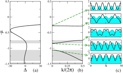
Figure 1: The structure of spectral bands of the linear periodic problem (4): (a) Trace of fundamental matrix $\Delta$ versus $\mu$; (b) Floquet exponent $k$ versus $\mu$; (c) Solid: Bloch waves at the band edges, as indicated by arrows; Dashed: potential $V(x)$. Parameters are $V_{0}=1$ and $d=10$.

When the spectral parameter $\mu$ is taken inside the spectral bands, i.e. $\mu\in\Sigma_{\rm band}$, the problem (4) has two linearly independent solutions in the form of Bloch waves,

$$\psi_{1}=\phi_{1}(x)e^{ik(\mu)x},\qquad\psi_{2}=\phi_{2}(x)e^{-ik(\mu)x},$$ (6)

where $\phi_{1,2}(x)$ are periodic functions and $k(\mu)$ is the Floquet exponent, which can be chosen inside the first Brillouin zone such that $0\leq k(\mu)\leq\frac{\pi}{d}$. The graph of $k(\mu)$ is shown in Fig. 1(b) for the first three spectral bands.

The spectral bands of the periodic potential (4) are described by the function $\Delta(\mu)$, which is the trace of fundamental matrix of solutions Eastham:1973:SpectralTheory

$$\Delta(\mu)=2\cos k(\mu)d,$$ (7)

The spectral bands are defined for $-2\leq\Delta(\mu)\leq 2$, which corresponds to propagating waves with real $k$. On the other hand, the waves become exponentially localized inside the gaps, where $|\Delta(\mu)|>2$ and ${\rm Im}(k)\neq 0$. A characteristic dependence $\Delta(\mu)$ is displayed in Fig. 1(a).

There are infinitely many spectral bands for a one-dimensional periodic potential $V(x)$, where $|\Delta(\mu)|\leq 2$ Eastham:1973:SpectralTheory . If $\Delta^{\prime}(\mu_{n})\neq 0$ at the band edge $\mu=\mu_{n}$, two adjacent spectral bands do not overlap, such that the corresponding band gap has a non-zero width. We consider the non-degenerate spectral band, such that $\Delta^{\prime}(\mu_{n})\neq 0$ at the end point $\mu=\mu_{n}$.

The even-numbered band edges $\mu=\mu_{2m}$, $m\geq 0$ correspond to periodic Bloch functions $\psi_{2m}(x+d)=\psi_{2m}(x)$, while the odd-numbered band edges $\mu=\mu_{2m-1}$, $m\geq 1$ correspond to anti-periodic Bloch functions $\psi_{2m-1}(x+d)=-\psi_{2m-1}(x)$. The Bloch functions $\psi_{n}(x)$ for the first five band edges $\mu=\mu_{0},\mu_{1},\mu_{3},\mu_{2},\mu_{4}$ are shown on Fig. 1(c).

We now demonstrate that the bifurcations of bound states and stationary gap solitons may occur when the two fundamental solutions $\psi_{1,2}(x)$ in (6) become linearly dependent. Since $\phi_{1}(x)e^{2ik(\mu)x}$ solves the same equation as $\phi_{2}(x)$ but it is not a periodic function of $x$, unless $k(\mu)=0\;\left({\rm mod}\left(\frac{2\pi}{d}\right)\right)$ or $k(\mu)=\frac{\pi}{d}\;\left({\rm mod}\left(\frac{2\pi}{d}\right)\right)$, the two solutions $\psi_{1,2}(x)$ are always linearly independent in the interior of the spectral bands $\mu\in\Sigma_{\rm band}$. On the other hand, the two solutions $\psi_{1,2}(x)$ become linearly dependent at the band edges $\mu=\mu_{n}$, since

$$\psi_{2m}(x)=\phi_{1}(x)=\phi_{2}(x)$$ (8)

and $k(\mu_{2m})=0\;\left({\rm mod}\left(\frac{2\pi}{d}\right)\right)$ at the even-numbered band edges, and

$$\psi_{2m-1}(x)=\phi_{1}(x)e^{\frac{\pi ix}{d}}=\phi_{2}(x)e^{\frac{-\pi ix}{d}}$$ (9)

and $k(\mu_{2m-1})=\frac{\pi}{d}\;\left({\rm mod}\left(\frac{2\pi}{d}\right)\right)$ at the odd-numbered band edges. The band edge $\mu=\mu_{n}$ has geometric multiplicity one with the only linearly independent Bloch function $\psi_{n}(x)$. The second, linearly independent solution of (4) at $\mu=\mu_{n}$ grows linearly in $x$. The band edge $\mu=\mu_{n}$ has however algebraic multiplicity two, since there exists a generalized Bloch function $\psi_{n}^{(1)}(x)$ that solves the derivative problem:

$$-(\psi_{n}^{(1)})^{\prime\prime}+V(x)\psi_{n}^{(1)}-\mu_{n}\psi_{n}^{(1)}=2\psi_{n}^{\prime}(x).$$ (10)

It follows from (10) that the generalized Bloch functions $\psi_{2m}^{(1)}(x)$ and $\psi_{2m-1}^{(1)}(x)$ are periodic and anti-periodic in $x$, respectively. We conclude that the band edges $\mu=\mu_{n}$ are the only bifurcation points of the linear spectrum $\mu\in\Sigma_{\rm band}$, associated with the periodic potential $V(x)$.

The band curvature near the band edge $\mu=\mu_{n}$ follows from the expansion of $\Delta(\mu)$ defined in (7):

$$\Delta(\mu_{n})+\Delta^{\prime}(\mu_{n})(\mu-\mu_{n})+{\rm O}(\mu-\mu_{n})^{2}$$

$$=(-1)^{n}\left(2-d^{2}(k-k_{n})^{2}+{\rm O}(k-k_{n})^{4}\right),$$ (11)

where $k_{2m}=0$ and $k_{2m-1}=\frac{\pi}{d}$. As a result, $\Delta(\mu_{n})=2(-1)^{n}$ and

$$\mu=\mu_{n}-\mu_{n}^{(2)}(k-k_{n})^{2}+{\rm O}(k-k_{n})^{4},$$ (12)

such that

$$\mu_{n}^{(2)}=\frac{d^{2}(-1)^{n}}{\Delta^{\prime}(\mu_{n})}.$$

The band curvatures $\mu_{n}^{(2)}$ can be expressed in terms of Bloch functions $\psi_{n}(x)$ and $\psi_{n}^{(1)}(x)$ at $\mu=\mu_{n}$. We use perturbation series expansions for fundamental solutions $\phi_{1,2}(x)$ near the band edges $\mu=\mu_{n}$:

$$\phi_{1,2}(x)e^{\pm ik_{n}x}=\psi_{n}(x)\pm i(k-k_{n})\psi_{n}^{(1)}(x)$$

$$-(k-k_{n})^{2}\psi_{n}^{(2)}(x)+{\rm O}(k-k_{n})^{3}.$$ (13)

The eigenvalue $\mu$ is expanded in the perturbation series (12). The second-order correction $\psi_{n}^{(2)}(x)$ satisfies the non-homogeneous linear equation:

$$-\left(\psi_{n}^{(2)}\right)^{\prime\prime}+V(x)\psi_{n}^{(2)}-\mu_{n}\psi_{n}^{(2)}$$

$$=2\left(\psi_{n}^{(1)}\right)^{\prime}+\left(1+\mu_{n}^{(2)}\right)\psi_{n}.$$ (14)

If $\phi_{1,2}(x)$ are periodic functions of $x$, the second-order correction $\psi_{n}^{(2)}(x)$ in the perturbation series (13) is periodic for $n=2m$ and anti-periodic for $n=2m-1$. By Fredholm Alternative, this condition is satisfied if the right-hand-side of (14) satisfies the constraint:

$$\left(1+\mu_{n}^{(2)}\right)\int_{0}^{d}\psi_{n}^{2}dx+2\int_{0}^{d}\psi_{n}\left(\psi_{n}^{(1)}\right)^{\prime}dx=0.$$ (15)

Therefore, the band curvature $\mu_{n}^{(2)}$ is expressed in terms of integrals of $\psi_{n}(x)$ and $\psi_{n}^{(1)}(x)$. The perturbation series expansions (12) and (13) can be continued algorithmically to the higher orders in powers of $(k-k_{n})$.

IV Bifurcations of gap solitons

Nonlinear bound states (gap solitons) of the NLS equation (1) are stationary solutions in the form:

$$\Psi(x,t)=\Phi_{s}(x)e^{-i\mu_{s}t},$$ (16)

where the real function $\Phi_{s}(x)$ decays to zero as $|x|\to\infty$ and satisfies the nonlinear problem,

$$-\Phi_{s}^{\prime\prime}+V(x)\Phi_{s}+\sigma\Phi_{s}^{3}=\mu_{s}\Phi_{s}.$$ (17)

When $\Phi_{s}(x)$ is small, the nonlinear potential $\sigma\Phi_{s}^{2}(x)$ acts as a perturbation term to the periodic potential $V(x)$. The perturbation term leads to bifurcation of gap solitons $\Phi_{s}(x)$ from the band edges $\mu=\mu_{n}$ of the linear band-gap spectrum. We study bifurcations of gap solitons with the multi-scale perturbation series expansions:

$$\mu_{s}=\mu_{n}+\epsilon^{2}\Delta_{n}+{\rm O}(\epsilon^{4}),$$ (18)

and

$$\Phi_{s}(x)=\epsilon\Phi_{\epsilon}(x;X),\quad X=\epsilon(x-x_{0}),\quad\epsilon\ll 1,$$ (19)

where

$$\Phi_{\epsilon}(x;X) = A_{n}(X)\psi_{n}(x)+\epsilon A_{n}^{\prime}(X)\psi_{n}^{(1)}(x)$$ (20)

$$+ \epsilon^{2}\phi_{s}^{(2)}(x;X)+{\rm O}(\epsilon^{3}).$$

Here $A_{n}(X)$ is a space-decaying bound state and $\psi_{n}(x)$ is the periodic or anti-periodic Bloch function. Parameter $x_{0}$ determines a location of $A_{n}(X)$ with respect to $\psi_{n}(x)$. The Bloch functions $\psi_{n}(x)$ and $\psi_{n}^{(1)}(x)$ are defined from the linear problems (4) and (10).

The second-order correction term $\phi_{s}^{(2)}(x;X)$ satisfies the linear non-homogeneous equation:

$$-\left(\phi_{s}^{(2)}\right)^{\prime\prime}+V(x)\phi_{s}^{(2)}-\mu_{n}\phi_{s}^{(2)}$$

$$=A_{n}^{\prime\prime}\left(\psi_{n}+2\left(\psi_{n}^{(1)}\right)^{\prime}\right)-\sigma A_{n}^{3}\psi_{n}^{3}+\Delta_{n}A_{n}\psi_{n}.$$ (21)

The secular growth of $\phi_{s}^{(2)}(x;X)$ in $x$ is removed if the right-hand-side of (21) satisfies the Fredholm condition, which reduces to the nonlinear equation for $A_{n}=A_{n}(X)$:

$$\mu_{n}^{(2)}A_{n}^{\prime\prime}+\chi_{n}^{(2)}A_{n}^{3}-\Delta_{n}A_{n}=0,$$ (22)

where

$$\chi_{n}^{(2)}=\sigma\frac{\int_{0}^{d}\psi_{n}^{4}dx}{\int_{0}^{d}\psi_{n}^{2}dx}.$$ (23)

Using the constraint (22), we represent the second-order correction term $\phi_{s}^{(2)}(x;X)$ in the form:

$$\phi_{s}^{(2)}(x;X)=A_{n}^{\prime\prime}(X)\psi_{n}^{(2)}(x)+A_{n}^{3}(X)\psi_{n}^{(nl2)}(x),$$ (24)

where $\psi_{n}^{(2)}(x)$ solves the non-homogeneous problem (14), while $\psi_{n}^{(nl2)}(x)$ solves the problem,

$$-\left(\psi_{n}^{(nl2)}\right)^{\prime\prime}+V(x)\psi_{n}^{(nl2)}-\mu_{n}\psi_{n}^{(nl2)}=\chi_{n}^{(2)}\psi_{n}-\sigma\psi_{n}^{3}.$$ (25)

The nonlinear equation (22) is just the stationary NLS equation, which has sech-solitons if ${\rm sign}(\mu_{n}^{(2)})={\rm sign}(\chi_{n}^{(2)})={\rm sign}(\Delta_{n})$. For the focusing nonlinearity, $\sigma=-1$, the sech-solitons bifurcate from all band edges, where $\mu_{n}^{(2)}<0$, such that $\Delta_{n}<0$. It follows from (12) that branches of gap solitons detach from all lower band edges downwards the corresponding band gaps [see Fig. 1(a)]. For the defocusing nonlinearity, $\sigma=+1$, the sech-solitons bifurcate from all band edges, where $\mu_{n}^{(2)}>0$, such that $\Delta_{n}>0$. Therefore, branches of gap solitons detach from all upper band edges upwards the corresponding band gaps [see Fig. 1(b)]. Branches of gap solitons are shown on Fig. 2 for $\sigma=-1$ near the band edges $\mu=\mu_{0}$, $\mu=\mu_{3}$, and $\mu=\mu_{4}$ and on Fig. 3 for $\sigma=+1$ near the band edges $\mu=\mu_{1}$ and $\mu=\mu_{2}$. The families of gap solitons have been found by solving the nonlinear eigenvalue problem (17) with a standard relaxation technique Press:1992:NumericalRecipes .

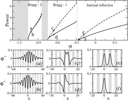
Figure 2: Bifurcations for the on-site and off-site gap solitons in a self-focusing medium ($\sigma=-1$). Top: the soliton power $P(\mu)=\int^{\infty}_{-\infty}\Phi_{s}^{2}(x;\mu)dx$ versus $\mu$. Solid: solitons centered at $x_{0}=0$, dashed: centered at $x_{0}=d/2$. (a-f): spatial profiles of gap solitons corresponding to marked points in the upper plot; shading marks the minima of the potential $V(x)$.

The sech-solitons of the nonlinear equation (22) are written explicitly in the form:

$$A_{n}(X)=a_{n}\;{\rm sech}(\kappa_{n}X),$$ (26)

where $a_{n}$ and $\kappa_{n}$ are found from equations,

$$\Delta_{n}-\kappa_{n}^{2}\mu_{n}^{(2)}=0,\qquad\chi_{n}^{(2)}a_{n}^{2}-2\kappa_{n}^{2}\mu_{n}^{(2)}=0,$$ (27)

provided that ${\rm sign}(\mu_{n}^{(2)})={\rm sign}(\chi_{n}^{(2)})={\rm sign}(\Delta_{n})$. The sech-type soliton envelopes (26) always have single-humped profile. Since $A_{n}(X)$ is the envelope of $\psi_{n}(x)$, the resulting nonlinear bound state $\Phi_{s}(x)$ has the oscillatory structure near the band edge $\mu_{s}=\mu_{n}$.

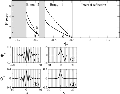
Figure 3: Bifurcations for the on-site and off-site gap solitons in a self-defocusing medium ($\sigma=+1$). Notations are the same as on Figure 2.

V Branches of gap solitons due to symmetry breaking

The absence of translational invariance along the $x$ direction, associated with the presence of the periodic potential, has an important effect on the soliton properties. For example, it was found that discrete solitons, bifurcating from the first band, can be centered at (on-site) or in-between (off-site) potential wells. In this Section, we demonstrate that two branches of gap solitons, bifurcating from all the bands, are centered at different positions in the periodic potential.

The gap soliton $\Phi_{s}(x)$ near the band edge $\mu_{s}=\mu_{n}$ is represented by the perturbation series expansions (18)–(20), provided that the formal series converges. Parameter $x_{0}$ in the ”slow” coordinate $X=\epsilon(x-x_{0})$ determines the location of the bound state $A_{n}(X)$ with respect to the Bloch function $\psi_{n}(x)$. We will show that only two values of $x_{0}$ on the period of $x$ secure convergence of the formal series, in the general case. Our analysis is equivalent to the construction of the Melnikov function, which gives the distance between separatrices in the nonlinear oscillator with a small, rapidly varying force Gelfreich:1997-227:PD ; Gelfreich:2000-266:PD . Zeros of the Melnikov function indicate values of $x_{0}$, where the separatrices intersect, so that a homoclinic orbit for the gap soliton exists in the nonlinear problem (17) with the periodic potential $V(x)$.

We will derive the Melnikov function Gelfreich:1997-227:PD ; Gelfreich:2000-266:PD with a simple but equivalent method. Derivative of the nonlinear equation (17) in $x$ results in the following third-order ODE:

$$-\Phi_{s}^{\prime\prime\prime}+V(x)\Phi_{s}^{\prime}-\mu_{s}\Phi_{s}^{\prime}+3\sigma\Phi_{s}^{2}\Phi_{s}^{\prime}+V^{\prime}(x)\Phi_{s}=0.$$ (28)

If the gap soliton $\Phi_{s}(x)$ exists, then it satisfies zero boundary conditions as $|x|\to\infty$. Multiplication of (28) by $\Phi_{s}(x)$ and integration it over $x$ result in the following constraint:

$$M_{s}(x_{0})=\int_{-\infty}^{\infty}V^{\prime}(x)\Phi_{s}^{2}(x)dx=0.$$ (29)

The function $M_{s}(x_{0})$ is the Melnikov function for existence of homoclinic orbits Gelfreich:1997-227:PD ; Gelfreich:2000-266:PD . The constraint (29) is always satisfied if the gap soliton $\Phi_{s}(x)$ and the potential $V(x)$ are symmetric with respect to the location of the central peak at $x=x_{0}$, such that $\Phi_{s}^{2}(x-x_{0})=\Phi_{s}^{2}(x_{0}-x)$ and $V^{\prime}(x-x_{0})=-V^{\prime}(x_{0}-x)$. More precise information on the constraint (29) can be obtained near the band edge $\mu_{s}=\mu_{n}$, where the perturbation series expansions (18)– (20) are valid. The function $\Phi_{\epsilon}(x;X)$ has the power series expansion in $\epsilon$, each term of which satisfies the squared-periodic boundary conditions in $x$,

$$\Phi^{2}_{\epsilon}(x+d;X)=\Phi^{2}_{\epsilon}(x;X),$$ (30)

and the decaying boundary conditions in $X$,

$$\lim_{|X|\to\infty}\Phi_{\epsilon}(x;X)=0.$$ (31)

We shall prove that $M_{s}(x_{0})$ is exponentially small in terms of $\epsilon$. To do so, we rewrite equation (28) for $\Phi_{\epsilon}(x;X)$, multiply it by $\Phi_{\epsilon}(x;X)$ and integrate the resulting equation over $x\in[0,d]$. Using the periodic boundary condition (30), we derive the relation,

$$\int_{0}^{d}V^{\prime}(x)\Phi_{\epsilon}^{2}(x;X)dx$$

$$=-2\epsilon\frac{\partial}{\partial X}\int_{0}^{d}\left(\Phi_{\epsilon,x}\right)^{2}dx-2\epsilon^{2}\frac{\partial}{\partial X}\int_{0}^{d}\Phi_{\epsilon,x}\Phi_{\epsilon,X}dx.$$ (32)

Using the decaying boundary condition (31), we prove that

$$\int_{-\infty}^{\infty}dX\int_{0}^{d}V^{\prime}(x)\Phi_{\epsilon}^{2}(x;X)dx=0.$$ (33)

As a result, the function $V^{\prime}(x)\Phi_{\epsilon}^{2}(x;X)$ is expanded in Fourier series in $x$ as

$$V^{\prime}(x)\Phi_{\epsilon}^{2}(x;X)=\sum_{m=-\infty}^{\infty}W_{n,m}(X;\epsilon)e^{\frac{2\pi imx}{d}},$$ (34)

such that $W_{n,-m}(X;\epsilon)=\overline{W_{n,m}}(X;\epsilon)$ and

$$\int_{-\infty}^{\infty}W_{n,0}(X;\epsilon)dX=0$$ (35)

at any order of $\epsilon$. The Fourier transform of $F(X)$ is defined by the standard integral:

$$\hat{F}(k)=\int_{-\infty}^{\infty}F(X)e^{ikX}dX.$$ (36)

The Melnikov function $M_{s}(x_{0})$ is then expanded with the use of the Fourier series (34) and the Fourier transform (36) in the form:

$$M_{s}(x_{0})=\epsilon\sum_{m=-\infty}^{\infty}\hat{W}_{n,m}\left(\frac{2\pi m}{\epsilon d};\epsilon\right)e^{\frac{2\pi imx_{0}}{d}}.$$ (37)

At the leading order, we have $W_{n,m}(X;0)=A_{n}^{2}(X)w_{n,m}^{(0)}$, where $w_{n,m}^{(0)}$ are coefficients in the Fourier series,

$$V^{\prime}(x)\psi_{n}^{2}(x)=\sum_{m=-\infty}^{\infty}w_{n,m}^{(0)}e^{\frac{2\pi imx}{d}}.$$ (38)

The zero-order term ($m=0$) in the series (37) is zero at any order of $\epsilon$, since the constraint (35) results in the condition: $\hat{W}_{n,0}(0;\epsilon)=0$. The higher-order terms with larger values of $|m|$ are exponentially smaller compared to the terms with smaller values of $|m|$ in the limit $\epsilon\to 0$, since $\hat{A}_{n}^{2}(k)$ is exponentially decaying in $k$. Therefore, using exponential asymptotics, we truncate the series (37) by the first-order terms ($m=\pm 1$) in the limit $\epsilon\to 0$:

$$M_{s}(x_{0})=\epsilon\Lambda_{1}\cos\left(\frac{2\pi x_{0}}{d}+{\rm arg}(w_{n,1}^{(0)})\right)+E_{1},$$ (39)

where

$$\Lambda_{1}=2|w_{n,1}^{(0)}|\hat{A}_{n}^{2}\left(\frac{2\pi}{\epsilon d}\right)$$

and

$$E_{1}={\rm O}\left(\epsilon^{2}\hat{A}_{n}^{2}\left(\frac{2\pi}{\epsilon d}\right)\right)+{\rm O}\left(\epsilon\hat{A}_{n}^{2}\left(\frac{4\pi}{\epsilon d}\right)\right).$$

Assuming that $\Lambda_{1}\neq 0$, we conclude from (39) that there are precisely two families of gap solitons bifurcating from two roots of the function $\cos(\frac{2\pi x_{0}}{d})$ on the period of $x_{0}$.

We now prove that, for the squared sine potential (2), the values of $\arg(w_{n,1}^{(0)})$ are the same for all band edges as $\arg(w_{n,1}^{(0)})=-\frac{\pi}{2}$. It is clear from (2) that $V(-x)=V(x)$ and $V^{\prime}(x)\geq 0$ for $0\leq|x|\leq d/2$, while all Bloch wave squared amplitudes are symmetric, such that $\psi_{n}^{2}(-x)=\psi_{n}^{2}(x)$. As a result, it follows from (38) that $\arg(w_{n,1}^{(0)})=-\frac{\pi}{2}$ and the two roots of $x_{0}$ occur at extremal points of $V(x)$: $x_{0}=0$ and $x_{0}=\frac{d}{2}$. The former (minimum) point corresponds to the on-site gap soliton, while the latter (maximum) point corresponds to the off-site gap soliton, in accordance with Figures 2 and 3.

When $\Lambda_{1}=0$ and $\hat{W}_{n,1}\left(\frac{2\pi}{\epsilon d};\epsilon\right)\neq 0$, higher powers of $\epsilon$ are generally non-zero in the first-order terms $(m=\pm 1)$, such that only two branches of gap solitons $\Phi_{s}(x)$ bifurcate in a general case. If the potential $V(x)$ is special such that $\hat{W}_{n,1}\left(\frac{2\pi}{\epsilon d};\epsilon\right)=0$ at any order of $\epsilon$ but $\hat{W}_{n,2}\left(\frac{4\pi}{\epsilon d};\epsilon\right)\neq 0$, the leading-order terms in the series (37) become second-order ($m=\pm 2$), such that four branches of gap solitons $\Phi_{s}(x)$ may bifurcate from four roots of the function $\cos(\frac{4\pi x_{0}}{d})$ on the period of $x_{0}$. We do not know whether any special potentials $V(x)$ may exist to hold the constraint $\hat{W}_{n,1}\left(\frac{2\pi}{\epsilon d};\epsilon\right)=0$ at any order of $\epsilon$.

VI Linear stability of gap solitons

Stability of solitons with respect to perturbations is an important problem for applications. Stable states act as attractors, and their excitation is weakly sensitive to noise or perturbations. On the other hand, unstable states tend to undergo dynamical transformations due to a rapid growth of initial perturbations, and this behavior may be useful, for example, for switching applications Morandotti:1999-2726:PRL .

We study the stability of gap solitons $\Phi_{s}(x)$ by considering the evolution of perturbed solution in the following form,

$$\psi(x,t)=e^{-i\mu_{s}t}\left[\Phi_{s}(x)+\left(u(x)+iw(x)\right)e^{\lambda t}\right.$$

$$+\left.\left(\overline{u(x)}+i\overline{w(x)}\right)e^{\bar{\lambda}t}\right].$$ (40)

We substitute Eq. (40) into the NLS equation (1) and perform its linearization with respect to the functions $(u,w)$ describing small-amplitude perturbations. Then, we obtain coupled linear eigenmode equations where $(u,w)$ is an eigenvector and $\lambda$ is an eigenvalue,

$${\cal L}_{1}u=-\lambda w,\qquad{\cal L}_{0}w=\lambda u.$$ (41)

Here ${\cal L}_{0}$ and ${\cal L}_{1}$ are Schrödinger operators with periodic and decaying potentials,

$${\cal L}_{0} = -\frac{d^{2}}{dx^{2}}+V(x)-\mu_{s}+\sigma\Phi_{s}^{2}(x),$$ (42)

$${\cal L}_{1} = -\frac{d^{2}}{dx^{2}}+V(x)-\mu_{s}+3\sigma\Phi_{s}^{2}(x).$$ (43)

We are interested in eigenvalues $\lambda$, which correspond to the spatially localized eigenvectors $(u,w)$ in $L^{2}({\mathbb{R}},{\mathbb{C}}^{2})$. If there exists an eigenvalue $\lambda$ with ${\rm Re}(\lambda)>0$, the gap soliton $\Phi_{s}(x)$ is spectrally unstable. On contrary, if all eigenvalues have ${\rm Re}(\lambda)=0$, the gap soliton is neutrally stable. Neutral stability can result in spectral instability due to resonances, embedded eigenvalues, and bifurcations of isolated eigenvalues with ${\rm Re}(\lambda)=0$. We have used an approach based on the Evans function for numerical calculation of the eigenvalues, the details are presented in Appendix A.

The stability problem (41) is written in terms of two Schrödinger operators ${\cal L}_{0}$ and ${\cal L}_{1}$ with periodic $V(x)$ and decaying $\sigma\Phi_{s}^{2}(x)$ potentials. At the band edge $\mu=\mu_{n}$, where $\Phi_{s}(x)\equiv 0$, the two Schrödinger operators coincide with the operator ${\cal L}_{s}$:

$${\cal L}_{s}=-\frac{d^{2}}{dx^{2}}+V(x)-\mu_{s}.$$ (44)

For $w=iu$ and $\lambda=i\Omega$, the spectral bands of the stability problem (41) occur at $\Omega+\mu_{s}\in\Sigma_{\rm band}$, i.e. at $\Omega\in[\mu_{0}-\mu_{s},\mu_{1}-\mu_{s}]\cup[\mu_{3}-\mu_{s},\mu_{2}-\mu_{s}]\cup...$. For the gap soliton bifurcating from the upper band edge $\mu_{s}=\mu_{n}$, the parameter $\mu_{s}$ satisfies the inequality: $\mu_{n}<\mu_{s}<\mu_{n+2}$, while for the gap soliton bifurcating from the lower band edge $\mu_{s}=\mu_{n}$, the parameter $\mu_{s}$ satisfies the inequality: $\mu_{n-2}<\mu_{s}<\mu_{n}$.

We demonstrate below that an important value which defines many stability properties is the energy of the spectral band, which is defined by

$$h=\langle u,{\cal L}_{1}u\rangle_{d}+\langle w,{\cal L}_{0}w\rangle_{d},$$ (45)

where the inner product $\langle\cdot,\cdot\rangle_{d}$ is defined for periodic Bloch functions on the period $x\in[0,d]$:

$$\langle f,g\rangle_{d}=\int_{0}^{d}\overline{f(x)}g(x)dx.$$ (46)

It is clear that $h_{m}=2(\mu_{m}-\mu_{n})\langle\psi_{m},\psi_{m}\rangle_{d}$ at $\epsilon=0$, where $h_{m}$ refers to the $m$-th band edge in the spectrum of ${\cal L}_{s}$ for $\mu_{s}=\mu_{n}$. All spectral bands of ${\cal L}_{s}$, which are lower with respect to $\mu_{s}=\mu_{n}$, become bands of negative energy for the gap soliton $\Phi_{s}(x)$, while all spectral bands of ${\cal L}_{s}$, which are upper with respect to $\mu_{s}=\mu_{n}$, become bands of positive energy for the gap soliton $\Phi_{s}(x)$.

The spectrum $\lambda$ of the stability problem (41) is double because of the inversion symmetry: $w=-iu$ and $\lambda=-i\Omega$. As a result, the bands of positive and negative energies of the operators ${\cal L}_{s}$ and $(-{\cal L}_{s})$ may overlap in the coupled spectrum (41) for the same values of $\lambda$.

The spectrum $\lambda$ of the problem (41) transforms when $\epsilon\neq 0$. A simple and stable transformation is a shift of spectral bands of ${\cal L}_{s}$ and $(-{\cal L}_{s})$ along the imaginary axis of $\lambda$ to the distance $|\mu_{s}-\mu_{n}|$. As a result, the origin $\lambda=0$ becomes isolated from the spectral bands of ${\cal L}_{s}$ and $(-{\cal L}_{s})$ for any $\epsilon\neq 0$.

Other transformations of the spectrum $\lambda$ are possible and may result in instabilities of gap solitons. These transformations are considered in Sections VII and  VIII.

VII Symmetry-breaking instability of gap solitons

In Sec. V, we have identified two families of on-site and off-site gap solitons, which have different positions with respect to the underlying potential. In this section, we demonstrate that one of these soliton families is unstable with respect to symmetry breaking. They tend to move across the potential and eventually transform into their stable counterparts which have a different position. These results generalize the previously found instability of off-site discrete solitons associated with the first band Morandotti:1999-2726:PRL .

More specifically, we show that the symmetry-breaking instability of gap solitons is defined by the sign of $M_{s}^{\prime}(x_{0})$. If $M_{s}^{\prime}(x_{0})>0$, then a pair of purely imaginary eigenvalues $\lambda$ in the stability problem (41) bifurcates from $\lambda=0$, and these internal modes describe oscillations of the perturbed soliton around the stable position $x=x_{0}$. On the other hand, if $M_{s}^{\prime}(x_{0})<0$, then a pair of real eigenvalues $\lambda$ bifurcates in the problem (41) and these exponentially growing instability modes characterize soliton motion away from the unstable location $x=x_{0}$. We note that these results are valid in the vicinity of gap edges, where the eigenvalues $\lambda$ are exponentially small in terms of the perturbation parameter $\epsilon$.

Due to the symmetry of the NLS equation (1), we have a non-empty kernel of the operator ${\cal L}_{0}$ for all $\epsilon$ along the family of the gap soliton $\Phi_{s}(x)$:

$${\cal L}_{0}\Phi_{\epsilon}(x;X)=0.$$ (47)

On the other hand, the gap soliton $\Phi_{s}(x)$ in the asymptotic representation (19) is parameterized by $x_{0}$ in the formal power series (20) in $\epsilon$. As a result, the kernel of the operator ${\cal L}_{1}$ is non-empty at all power orders of $\epsilon^{n}$:

$${\cal L}_{1}U_{\epsilon}=0(\epsilon^{n}),\qquad U_{\epsilon}=\frac{\partial\Phi_{\epsilon}(x;X)}{\partial X}.$$ (48)

The zero eigenvalue of ${\cal L}_{1}$ is destroyed beyond the powers of $\epsilon$, since the gap soliton $\Phi_{s}(x)$ is not parameterized by $x_{0}$, values of which are fixed by roots of the Melnikov function (29). We show in Appendix B that the zero eigenvalue of ${\cal L}_{1}$, associated with the eigenfunction $U_{\epsilon}(x)$, shifts according to the quadratic form:

$$\left(U_{\epsilon},{\cal L}_{1}U_{\epsilon}\right)=\frac{1}{2\epsilon^{4}}M_{s}^{\prime}(x_{0}),$$ (49)

where the quadratic form is defined for decaying functions on the whole line of $x$:

$$\left(f,g\right)=\int_{-\infty}\overline{f(x)}g(x)dx.$$ (50)

According to the standard perturbation theory Horn:1985:MatrixAnalysis , the quadratic form in (49) determines the shift of the zero eigenvalue of ${\cal L}_{1}$, associated with the eigenfunction $U_{\epsilon}(x)$. When $M_{s}^{\prime}(x_{0})>0$, the zero eigenvalue of ${\cal L}_{1}$ becomes positive, while when $M_{s}^{\prime}(x_{0})<0$, the zero eigenvalue of ${\cal L}_{1}$ becomes negative. We show that a small negative eigenvalue of ${\cal L}_{1}$ results in a small real positive eigenvalue $\lambda$ of the stability problem (41), while a small positive eigenvalue ${\cal L}_{1}$ results in a pair of small imaginary eigenvalues $\lambda$.

A small eigenvalue $\lambda=\lambda_{\epsilon}$, corresponding to the eigenfunction $u_{\epsilon}(x)$, can be found from the problem:

$${\cal L}_{1}u_{\epsilon}=-\lambda_{\epsilon}^{2}{\cal L}_{0}^{-1}u_{\epsilon},$$ (51)

or equivalently, from the Rayleigh quotient:

$$\lambda_{\epsilon}^{2}=-\frac{\left(u_{\epsilon},{\cal L}_{1}u_{\epsilon}\right)}{\left(u_{\epsilon},{\cal L}_{0}^{-1}u_{\epsilon}\right)}.$$ (52)

The quadratic form $\left(u_{\epsilon},{\cal L}_{0}^{-1}u_{\epsilon}\right)$ exists if $(\Phi_{\epsilon},u_{\epsilon})=0$, as follows from (47). Since $(\Phi_{\epsilon},U_{\epsilon})={\rm O}(\epsilon^{n})$ and ${\cal L}_{1}U_{\epsilon}={\rm O}(\epsilon^{n})$ at all power orders of $\epsilon^{n}$, we conclude that

$$u_{\epsilon}(x)=U_{\epsilon}(x)+E_{\epsilon},$$ (53)

where $E_{\epsilon}$ is exponentially small in terms of $\epsilon$. We shall prove that

$$\left(u_{\epsilon},{\cal L}_{0}^{-1}u_{\epsilon}\right)=\frac{1}{4\epsilon^{2}}\left(\Phi_{\epsilon},\Phi_{\epsilon}\right)+{\rm O}\left(\frac{1}{\epsilon}\right),$$ (54)

such that $\left(u_{\epsilon},{\cal L}_{0}^{-1}u_{\epsilon}\right)>0$ at the leading order. It follows from the nonlinear problem (17) that

$${\cal L}_{0}X\Phi_{\epsilon}(x;X)=-2\epsilon\frac{\partial\Phi_{\epsilon}(x;X)}{\partial x}-2\epsilon^{2}\frac{\partial\Phi_{\epsilon}(x;X)}{\partial X}.$$ (55)

As a result, we have

$$-\frac{1}{2\epsilon^{2}}\left(\frac{\partial\Phi_{\epsilon}}{\partial X},X\Phi_{\epsilon}\right)$$

$$=\left(\frac{\partial\Phi_{\epsilon}}{\partial X},{\cal L}_{0}^{-1}\frac{\partial\Phi_{\epsilon}}{\partial X}\right)+\frac{1}{\epsilon}\left(\frac{\partial\Phi_{\epsilon}}{\partial X},{\cal L}_{0}^{-1}\frac{\partial\Phi_{\epsilon}}{\partial x}\right).$$ (56)

Solution of the inhomogeneous problem,

$${\cal L}_{0}V_{\epsilon}=\frac{\partial\Phi_{\epsilon}}{\partial x},$$ (57)

exists at all power orders of $\epsilon^{n}$, since the right-hand-side of (57) is orthogonal to $\Phi_{\epsilon}$ at all power orders of $\epsilon^{n}$. Therefore, the quadratic form $(U_{\epsilon},V_{\epsilon})$ has a regular power series in $\epsilon$, starting with the zero-order term. Since

$$-\frac{1}{2\epsilon^{2}}\left(\frac{\partial\Phi_{\epsilon}}{\partial X},X\Phi_{\epsilon}\right) = \frac{1}{4\epsilon^{2}}\left(\Phi_{\epsilon},\Phi_{\epsilon}\right)$$ (58)

$$- \frac{1}{4\epsilon^{2}}\int_{-\infty}^{\infty}\frac{\partial}{\partial X}\left(X\Phi^{2}_{\epsilon}\right)dx,$$

and the second term is exponentially small in $\epsilon$, we have (54) at the leading order, such that the Rayleigh quotient (52) is given in the leading order by:

$$\lambda^{2}_{\epsilon}\approx-\frac{2M_{s}^{\prime}(x_{0})}{\epsilon^{2}\left(\Phi_{\epsilon},\Phi_{\epsilon}\right)}.$$ (59)

It follows from (59) that a negative eigenvalue of ${\cal L}_{1}$ for $M_{s}^{\prime}(x_{0})<0$ results in a small positive eigenvalue $\lambda_{\epsilon}$ in the stability problem (41).

The exponentially small correction of the function $M_{s}(x_{0})$ is given by the expansion (39), where ${\rm arg}\left(w_{n,1}^{(0)}\right)=-\frac{\pi}{2}$ for the square-sine potential (2). Therefore, $M_{s}^{\prime}(x_{0})>0$ for $x_{0}=0$ and $M_{s}^{\prime}(x_{0})<0$ for $x_{0}=\frac{d}{2}$. In the former case, the gap soliton $\Phi_{s}(x)$ is located at the minimum point of $V(x)$ and it has a pair of small imaginary eigenvalues $\lambda$. In the latter case, the gap soliton $\Phi_{s}(x)$ is located at the maximum point of $V(x)$ and it is unstable with a small real positive eigenvalue $\lambda$. Fig. 4 shows unstable eigenvalues, splitting from zero eigenvalues, for the branches of gap solitons with $x_{0}=\frac{d}{2}$. We note that stability of on-site and off-site solitons can be interchanged in more complex potentials, such as binary superlattices Sukhorukov:2003-2345:OL . Additionally, stability can change deep inside the gap, where the asymptotic analysis is not applicable Gorbach:2004-77:EPD .

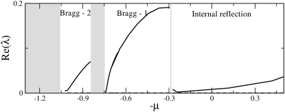
Figure 4: Eigenvalues corresponding to symmetry-breaking instabilities of gap solitons centered at $x_{0}=d/2$ (shown with dashed lines in Fig. 2) for $\sigma=-1$.

Asymptotic results for NLS solitons in the lowest semi-infinite band gap in the focusing case ($\sigma=-1$) were obtained recently by Kapitula Kapitula:2001-186:PD in the limit $V(x)\to 0$. Branches of NLS solitons $\Phi_{s}(x)=\Phi_{\rm NLS}(x)=\sqrt{2\mu_{s}}\;{\rm sech}(\sqrt{2\mu_{s}}(x-x_{0}))$ in the small periodic potential function $V(x)$ are defined by zeros of the function $M_{s}(x_{0})$, given by (29) with $\Phi_{s}=\Phi_{\rm NLS}(x)$. Stability of branches of NLS solitons is defined by the derivative $M_{s}^{\prime}(x_{0})$, such that the NLS solitons bifurcating from the minimum points of $V(x)$ are stable, while the NLS solitons bifurcating from the maximum points of $V(x)$ are unstable. We note that the opposite conclusion is drawn in Ref. Kapitula:2001-186:PD , due to an elementary sign error.

VIII Internal modes and oscillatory instabilities of gap solitons

Apart from symmetry-breaking instabilities analyzed in the previous section, we demonstrate that gap solitons can exhibit a different type, so-called oscillatory instabilities. Such instabilities can occur due to a resonance between the modes corresponding to the edges of the gap in which soliton is localized, as was demonstrated in the case of a narrow gap when the coupled-mode equations are applicable Barashenkov:1998-5117:PRL . However, the coupled-mode theory described only an isolated band-gap, whereas it was found that oscillatory instability can occur due to resonance between different gaps Sukhorukov:2001-83901:PRL ; Sukhorukov:2003-2345:OL . Such resonances can result in energy redistribution between the gaps and a formation of breathing structures, as was recently demonstrated experimentally Neshev:nlin.PS/0311059:ARXIV . In this section, we present a systematic analysis of such instabilities, and show that they appear when a side-band associated with the inter-gap resonances falls outside a band-gap.

Oscillatory modes and instabilities are characterized by eigenvalues $\lambda$ with non-zero imaginary part of the stability problem (41) for $\epsilon\neq 0$. First, we show that new imaginary eigenvalues $\lambda$ with decaying eigenvectors $(u,w)$ bifurcate from the band edges $\lambda=i(\mu_{m}-\mu_{n})$ of the same polarity as the band edge $\mu_{s}=\mu_{n}$. Bifurcations of internal modes occur generally at the order of ${\rm O}(\epsilon^{2})$, if $\mu_{m}\neq\mu_{n}$. These eigenvalues are referred to as the internal modes of gap solitons Pelinovsky:1998-121:PD ; Kivshar:1998-5032:PRL , and in our case such modes appear due to a resonance between the gap edges $m$ and $n$. Such resonances are possible because a soliton induces an effective waveguide, which can support localized modes in other gaps Cohen:2003-113901:PRL ; Sukhorukov:2003-113902:PRL . In Fig. 5, we show three modes of operator ${\cal L}_{0}$ supported in the semi-infinite gap near the edge $\mu=\mu_{0}$ by a gap soliton existing in the gap near the edge $\mu=\mu_{2}$ in the case of a self-focusing nonlinearity ($\sigma=-1$).

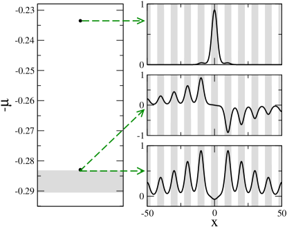
Figure 5: Linear guided modes of operator ${\cal L}_{0}$ in the semi-infinite band-gap for a gap soliton shown in Fig. 2(d). Left: eigenvalues marked with dots (second and third ones are indistinguishable within the picture scale); Right: corresponding mode profiles.

Second, we show that resonance between internal modes of the operator ${\cal L}_{s}$ and the bands of the inverted spectrum of $(-{\cal L}_{s})$ occurs if the bifurcating internal mode of ${\cal L}_{s}$ becomes embedded into the spectral band of $(-{\cal L}_{s})$. When it happens, embedded internal modes bifurcate generally to complex eigenvalues $\lambda$, leading to oscillatory instabilities of the gap soliton $\Phi_{s}(x)$. Resonant bifurcations of complex eigenvalues $\lambda$ occur generally at order of ${\rm O}(\epsilon^{4})$.

Third, we show that the internal mode of ${\cal L}_{s}$ may occur near the band edge of the inverted spectrum of $(-{\cal L}_{s})$. In this case, bifurcations of isolated, embedded, and complex eigenvalues are all possible at the order of ${\rm O}(\epsilon^{2})$, depending on the configuration of the spectral bands of ${\cal L}_{s}$ and $(-{\cal L}_{s})$.

Finally, we show that at most one internal mode can bifurcate from the band edge, which is closest to the zero eigenvalue. This bifurcation occurs generally at the order of ${\rm O}(\epsilon^{4})$.

We emphasize that bifurcations of new eigenvalues may not generally occur in higher orders of $\epsilon$, since the band edges of the spectrum of ${\cal L}_{1}$ and ${\cal L}_{0}$ with $\Phi_{s}(x)\neq 0$ do not support resonances in a generic case. Bifurcations of new eigenvalues may occur far from the limit $\epsilon=0$, when the spectral bands of the linearized operator get additional resonances at the band edges or in the interior points. Bifurcations of the existing eigenvalues may also occur far from the limit $\epsilon=0$, if the existing eigenvalues coalesce with each other or with the spectral bands.

VIII.1 Non-resonant bifurcations of internal modes

Let $n$ be the index of the band edge $\mu_{s}=\mu_{n}$ where the gap soliton $\Phi_{s}(x)$ bifurcates from. We consider a different band edge of the stability problem (41) with $\lambda=i(\mu_{m}-\mu_{n})$, such that $m\neq n$. We assume that the $m$-th band edge of the spectrum of ${\cal L}_{s}$ is located in a band gap of the inverted spectrum of $(-{\cal L}_{s})$, such that $2\mu_{n}-\mu_{m}\notin\Sigma_{\rm band}$. Using the same perturbation series expansions (18) and (20), we expand solutions of the stability problem (41) in the perturbation series:

$$u=B_{m}(X)\psi_{m}(x)+\epsilon B_{m}^{\prime}(X)\psi_{m}^{(1)}(x)$$

$$+\epsilon^{2}u_{m}^{(2)}(x,X)+{\rm O}(\epsilon^{3}),$$ (60)

$$w=i\left[B_{m}(X)\psi_{m}(x)+\epsilon B_{m}^{\prime}(X)\psi_{m}^{(1)}(x)\right.$$

$$+\left.\epsilon^{2}w_{m}^{(2)}(x,X)+{\rm O}(\epsilon^{3})\right],$$ (61)

and

$$\lambda=i\left[\mu_{m}-\mu_{s}+\epsilon^{2}\Omega_{m}+{\rm O}(\epsilon^{4})\right],$$ (62)

where the second-order correction terms $(u_{m}^{(2)},w_{m}^{(2)})$ solve the non-homogeneous system:

$${\cal L}_{s}u_{m}^{(2)}+(\mu_{s}-\mu_{m})w_{m}^{(2)}=B_{m}^{\prime\prime}\left(\psi_{m}+2\left(\psi_{m}^{(1)}\right)^{\prime}\right)$$

$$+\Omega_{m}B_{m}\psi_{m}-3\sigma A_{n}^{2}B_{m}\psi_{n}^{2}\psi_{m},$$ (63)

$${\cal L}_{s}w_{m}^{(2)}+(\mu_{s}-\mu_{m})u_{m}^{(2)}=B_{m}^{\prime\prime}\left(\psi_{m}+2\left(\psi_{m}^{(1)}\right)^{\prime}\right)$$

$$+\Omega_{m}B_{m}\psi_{m}-\sigma A_{n}^{2}B_{m}\psi_{n}^{2}\psi_{m}.$$ (64)

Under the constraint that $(2\mu_{s}-\mu_{m})\notin\Sigma_{\rm band}$, the second-order corrections $(u_{m}^{(2)},w_{m}^{(2)})$ are periodic or anti-periodic functions of $x$, when a single Fredholm condition is satisfied. The Fredholm condition takes the form of the eigenvalue problem for $\Omega_{m}$:

$$\mu_{m}^{(2)}B_{m}^{\prime\prime}+2\chi_{nm}^{(2)}A_{n}^{2}(X)B_{m}-\Omega_{m}B_{m}=0,$$ (65)

where

$$\chi_{nm}^{(2)}=\sigma\frac{\int_{0}^{d}\psi_{n}^{2}\psi_{m}^{2}dx}{\int_{0}^{d}\psi_{m}^{2}dx}.$$ (66)

We note that Eq. (65) describes the linear modes supported by a soliton-induced waveguide in other gaps. The linear problem (65) is a Schrödinger equation with the solvable potential (26). There is at least one isolated eigenvalue if ${\rm sign}(\mu_{m}^{(2)})={\rm sign}(\chi_{nm}^{(2)})={\rm sign}(\Omega_{m})$. In this case, the lowest eigenvalue and eigenfunction of the problem (65) can be found explicitly as

$$\Omega_{m}=\kappa_{n}^{2}\mu_{m}^{(2)}s_{m}^{2},\qquad B_{m}={\rm sech}^{s_{m}}(\kappa_{n}X),$$ (67)

where $s_{m}$ solves the quadratic equation,

$$s_{m}(s_{m}+1)=\frac{4\mu_{n}^{(2)}\chi_{nm}^{(2)}}{\mu_{m}^{(2)}\chi_{n}^{(2)}}.$$ (68)

Isolated eigenvalues $\Omega_{m}$ of the problem (65), when exist, correspond to internal modes $\lambda$ in the perturbation series (62), bifurcating in the band gaps of the operators ${\cal L}_{s}$ and $(-{\cal L}_{s})$ from the band edge $\lambda=i(\mu_{m}-\mu_{n})$. When ${\rm sign}(\mu_{m}^{(2)})=-{\rm sign}(\chi_{nm}^{(2)})$, the linear problem (65) does not have any isolated eigenvalues. Since ${\rm sign}(\chi_{nm}^{(2)})={\rm sign}(\chi_{n}^{(2)})={\rm sign}(\sigma)$, we notice that all band edges $\mu=\mu_{n}$ that support bifurcations of gap solitons in the nonlinear problem (17), support also bifurcations of internal modes $\lambda$ in the spectrum of a selected $n$-th gap soliton. In the focusing case, $\sigma=-1$, all lower band edges generate internal modes $\lambda$ downwards the corresponding band gaps, i.e. $\mu_{m}^{(2)}<0$ and $\Omega_{m}<0$. In the defocusing case, $\sigma=+1$, all upper band edges generate internal modes $\lambda$ upwards the corresponding band edges, i.e. $\mu_{m}^{(2)}>0$ and $\Omega_{m}>0$.

It is surprising that more than one internal mode $\lambda$ could be generated near the band edge $\lambda=i(\mu_{m}-\mu_{n})$. In the case of no periodic potential $V(x)=0$, perturbations of NLS solitons generate at most one internal mode Kivshar:1998-5032:PRL ; Kapitula:2001-533:NLN . On the other hand, perturbations of gap solitons in the coupled-mode equations (derived for small $V(x)$ in the narrow band gap of the first resonance) may generate several internal modes and complex eigenvalues Barashenkov:1998-5117:PRL ; Kapitula:2002-1117:SJMA . In the case of finite potential $V(x)$, the number of internal modes depends on the depth of the squared sech potential in the eigenvalue problem (65), which is determined by parameters of the band curvatures $\mu_{n}^{(2)}$ and $\mu_{m}^{(2)}$ and by the nonlinearity coefficients $\chi_{n}^{(2)}$ and $\chi_{nm}^{(2)}$.

VIII.2 Resonant bifurcations of complex eigenvalues

According to the general expression (40), eigenvalues $\lambda$ with non-zero imaginary part describe soliton oscillations, which are associated with the appearance of two side-band spatial frequencies $\mu+{\rm Im}(\lambda)$ and $\mu-{\rm Im}(\lambda)$. Gap solitons are spectrally stable for small values of $\epsilon\neq 0$ with respect to a particular resonant oscillation if both of the side-bands fall inside the gaps of the linear spectrum, whereas an oscillatory instability may arise when one side-band appears inside a linear transmission band Sukhorukov:2001-83901:PRL ; Sukhorukov:2003-2345:OL . This general behavior is illustrated in Fig. 6, where the real part of the eigenvalue is non-zero indicating a presence of the oscillatory instability when the lower side-band is inside the transmission band of the inverted spectrum. However, the instability is suppressed when the side-band moves inside the band gap. The instability shown in Fig. 6 appears due to a resonant coupling between a gap soliton marked ”d” in Fig. 2, and its own fundamental guided mode in the first gap shown in Fig. 5. The characteristic profiles of instability modes are presented in Fig. 7. The top row shows the perturbation $u+iw$, which corresponds to higher spatial frequency $\mu+{\rm Im}(\lambda)$ according to Eq. (40), and we indeed see that this mode closely matches the guided mode profile [cf. Fig. 5] in agreement with the asymptotic expressions (60) and (61). On the other hand, the bottom row of Fig. 7 shows the low-frequency component, which describes the radiation waves emitted by the soliton when $\mu-{\rm Im}(\lambda)$ is inside the transmission band. We note however that the rate of such radiation may be very small, allowing for the existence of long-lived oscillating, or breathing states, such as shown in Fig. 8. Similar effects may occur due to a resonance with higher-order guided modes, as shown in Figs. 9-11. One important difference is that the associated breathing states can have different symmetries for various excited modes, cf. Figs. 8 and 11.

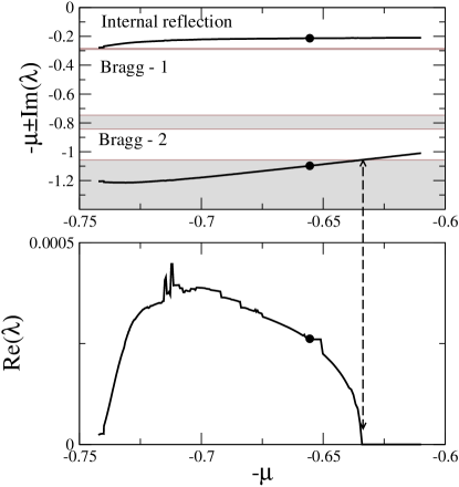
Figure 6: Eigenvalues corresponding to a resonance of a gap soliton (marked ”d” in Fig. 2) with its fundamental guided mode in the semi-infinite band-gap.

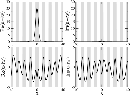
Figure 7: Profiles of linear modes corresponding to a resonance in Fig. 6.

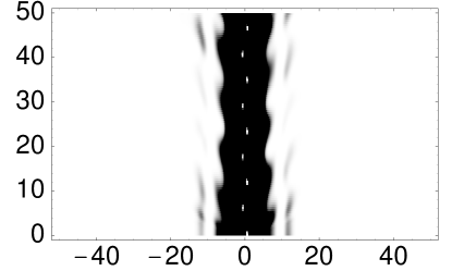
Figure 8: Evolution of a soliton perturbed by a linear mode corresponding to Fig. 7.

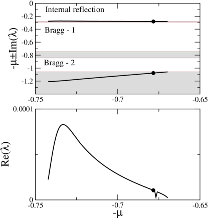
Figure 9: Eigenvalues corresponding to a resonance of a gap soliton (marked ”d” in Fig. 2) with its higher-order guided mode in the semi-infinite band-gap.

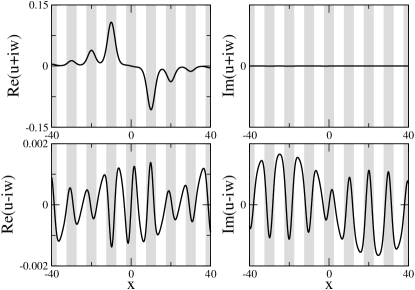
Figure 10: Profiles of linear modes corresponding to a resonance in Fig. 9.

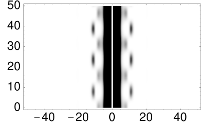
Figure 11: Evolution of a soliton perturbed by a linear mode corresponding to Fig. 10.

In mathematical terms, stability requires that all internal modes detaching from the band edges $\lambda=i(\mu_{m}-\mu_{n})$ reside inside the band gaps of the inverted operator $(-{\cal L}_{s})$, and the zero eigenvalue of ${\cal L}_{1}$ shifts to small imaginary eigenvalues $\lambda$. When an internal mode is embedded into a spectral band of the inverted operator $(-{\cal L}_{s})$, oscillatory instability of the gap soliton $\Phi_{s}(x)$ may arise for small values of $\epsilon\neq 0$. Embedded imaginary eigenvalues $\lambda$ are known to be structurally unstable with respect to small perturbations and, provided that their energy is opposite with respect to the energy density of the spectral band, they bifurcate into complex eigenvalues $\lambda$ Tsai:2002-1629:IMRN . By construction, resonance of internal modes of ${\cal L}_{s}$ with spectral bands of $(-{\cal L}_{s})$ is only possible if the internal mode, detaching from the band edge $\lambda=i(\mu_{m}-\mu_{s})$, has the opposite energy signature with respect to the energy signature of the inverted spectral band $\mu_{r}=2\mu_{n}-\mu_{m}\in\Sigma_{\rm band}$, such that $\lambda=i(\mu_{m}-\mu_{n})=i(\mu_{n}-\mu_{r})$. Therefore, all embedded imaginary eigenvalues in the linearized stability problem (41) are expected to bifurcate to complex eigenvalues $\lambda$ in a generic case.

We prove in Appendix C that, provided that $\mu_{r}=2\mu_{n}-\mu_{m}\in\Sigma_{\rm band}$, we have

$${\rm Re}(\lambda)=\epsilon^{4}\Gamma_{m}+{\rm O}(\epsilon^{5}),\qquad\Gamma_{m}\geq 0,$$ (69)

where $\lambda$ is the eigenvalue of the bifurcating internal mode, given by (62). In a generic case, when $\Gamma_{m}\neq 0$, the embedded imaginary eigenvalue $\lambda$ bifurcates to the unstable domain ${\rm Re}(\lambda)>0$ and leads to oscillatory instabilities of the gap soliton $\Phi_{s}(x)$.

VIII.3 Marginal bifurcations of internal modes and complex eigenvalues

A marginal case between non-resonant and resonant bifurcations occurs when internal modes detaching from the band edge $\lambda=i(\mu_{m}-\mu_{n})$ are located in the neighborhood of the band edge $\lambda=i(\mu_{n}-\mu_{k})$ of the inverted spectrum. We assume here that $\mu_{m}$, $\mu_{k}$, and $\mu_{s}$ satisfy the resonance condition within the mismatch of order ${\rm O}(\epsilon^{2})$:

$$\mu_{m}+\mu_{k}-2\mu_{s}=\epsilon^{2}\nu_{mk}.$$ (70)

In this marginal case, we expand the eigenvalue $\lambda$ and the eigenfunction $(u,w)$ of the linearized stability problem (41) in the modified perturbation series,

$$u=u_{mk}^{(0)}(x;X)+\epsilon u_{mk}^{(1)}(x;X)$$

$$+\epsilon^{2}u_{mk}^{(2)}(x;X)+{\rm O}(\epsilon^{3}),$$ (71)

$$w=i\left[w_{mk}^{(0)}(x;X)+\epsilon w_{mk}^{(1)}(x;X)\right.$$

$$+\left.\epsilon^{2}w_{mk}^{(2)}(x;X)+{\rm O}(\epsilon^{3})\right],$$ (72)

and

$$\lambda=i\left[\mu_{m}-\mu_{s}+\epsilon^{2}\Omega_{mk}+{\rm O}(\epsilon^{4})\right],$$ (73)

where

$$u_{mk}^{(0)} = B_{m}(X)\psi_{m}(x)+C_{k}(X)\psi_{k}(x),$$

$$u_{mk}^{(1)} = B_{m}^{\prime}(X)\psi_{m}^{(1)}(x)+C_{k}^{\prime}(X)\psi_{k}^{(1)}(x),$$

$$w_{mk}^{(0)} = B_{m}(X)\psi_{m}(x)-C_{k}(X)\psi_{k}(x),$$

$$w_{mk}^{(1)} = B_{m}^{\prime}(X)\psi_{m}^{(1)}(x)-C_{k}^{\prime}(X)\psi_{k}^{(1)}(x).$$

The second-order correction terms $(u_{mk}^{(2)},w_{mk}^{(2)})$ solve the system:

$${\cal L}_{s}u_{mk}^{(2)}+(\mu_{s}-\mu_{m})w_{mk}^{(2)} = F^{(2)},$$

$${\cal L}_{s}w_{mk}^{(2)}+(\mu_{s}-\mu_{m})u_{mk}^{(2)} = G^{(2)},$$ (74)

where

$$F^{(2)} = B_{m}^{\prime\prime}\left(\psi_{m}+2\left(\psi_{m}^{(1)}\right)^{\prime}\right)+C_{k}^{\prime\prime}\left(\psi_{k}+2\left(\psi_{k}^{(1)}\right)^{\prime}\right)$$

$$+ \Omega_{mk}\left(B_{m}\psi_{m}-C_{k}\psi_{k}\right)-\nu_{mk}C_{k}\psi_{k}$$

$$- 3\sigma A_{n}^{2}\psi_{n}^{2}\left(B_{m}\psi_{m}+C_{k}\psi_{k}\right),$$

$$G^{(2)} = B_{m}^{\prime\prime}\left(\psi_{m}+2\left(\psi_{m}^{(1)}\right)^{\prime}\right)-C_{k}^{\prime\prime}\left(\psi_{k}+2\left(\psi_{k}^{(1)}\right)^{\prime}\right)$$

$$+ \Omega_{mk}\left(B_{m}\psi_{m}+C_{k}\psi_{k}\right)+\nu_{mk}C_{k}\psi_{k}$$

$$- \sigma A_{n}^{2}\psi_{n}^{2}\left(B_{m}\psi_{m}-C_{k}\psi_{k}\right).$$

Because of the resonance condition (70), the second-order corrections $(u_{mk}^{(2)},w_{mk}^{(2)})$ are periodic or anti-periodic functions of $x$ if two Fredholm conditions are satisfied. The two Fredholm conditions take the form of a coupled eigenvalue problem for $\Omega_{mk}$:

$$\mu_{m}^{(2)}B_{m}^{\prime\prime}+A_{n}^{2}(X)\left(2\chi_{nm}^{(2)}B_{m}+\chi_{nmk}^{(2)}C_{k}\right)=\Omega_{mk}B_{m},$$

$$\mu_{k}^{(2)}C_{k}^{\prime\prime}+A_{n}^{2}(X)\left(\chi_{nkm}^{(2)}B_{m}+2\chi_{nk}^{(2)}C_{k}\right)=$$

$$\qquad\qquad\qquad-\left(\nu_{mk}+\Omega_{mk}\right)C_{k},$$ (75)

where $\chi_{nm}^{(2)}$ is defined in (66), while $\chi_{nmk}^{(2)}$ and $\chi_{nkm}^{(2)}$ are defined as

$$\chi_{nmk}^{(2)}=\sigma\frac{\int_{0}^{d}\psi_{n}^{2}\psi_{m}\psi_{k}dx}{\int_{0}^{d}\psi_{m}^{2}dx}.$$ (76)

The coupled eigenvalue problem (VIII.3)–(75) is not self-adjoint and therefore the eigenvalues $\Omega_{mk}$ could be complex-valued.

We assume that ${\rm sign}(\mu_{m}^{(2)})={\rm sign}(\chi_{nm}^{(2)})$ such that the first equation (VIII.3) with $C_{k}\equiv 0$ has at least one internal mode for ${\rm sign}(\Omega_{mk})={\rm sign}(\mu_{m}^{(2)})$. For convenience, we consider here the defocusing case $\sigma=1$, when $\chi_{nm}^{(2)}>0$ and $\mu_{m}^{(2)}>0$. In this case, the internal mode of the first equation (VIII.3) with $C_{k}\equiv 0$ exists for $\Omega_{mk}>0$, while the spectral band is located for negative values of $\Omega_{mk}$. There are two particular cases, depending on whether $\mu_{k}^{(2)}>0$ or $\mu_{k}^{(2)}<0$.

In the case $\mu_{k}^{(2)}<0$, the second equation (75) with $B_{m}\equiv 0$ does not have any internal modes, while the spectral band is located below the value $\Omega_{mk}\leq-\nu_{mk}$. When $\nu_{mk}\gg 1$, internal modes in the component $B_{m}$ for $\Omega_{mk}>0$ are not affected by the spectral band in the component $C_{k}$, since the following estimate holds for finite $\Omega_{mk}$ and large $\nu_{mk}$:

$$C_{k}=-\frac{\chi_{nkm}^{(2)}}{\nu_{mk}}A_{n}^{2}(X)B_{m}+{\rm O}\left(\frac{1}{\nu_{mk}^{2}}\right).$$ (77)

When the value of $\nu_{mk}$ decreases and becomes negative, all internal modes in the component $B_{m}$ become embedded into the spectral band in the component $C_{k}$. The embedded eigenvalues $\Omega_{mk}$ bifurcate as complex eigenvalues $\Omega_{mk}$ due to Fermi golden rule as in Tsai:2002-1629:IMRN .

In the case of $\mu_{k}^{(2)}>0$, the second equation (75) with $B_{m}\equiv 0$ has at least one internal mode for $\nu_{mk}+\Omega_{mk}<0$, while the spectral band is located above the value $\Omega_{mk}\geq-\nu_{mk}$. When $\nu_{mk}\ll-1$, all internal modes in the component $B_{m}$ for $\Omega_{mk}>0$ and those in the component $C_{k}$ for $\nu_{mk}+\Omega_{mk}<0$ are located in the gap between the two spectral bands. The internal modes in the component $B_{m}$ are not affected by the spectral band in the component $C_{k}$, since $C_{k}$ is small according to the expansion (77). On the other hand, the internal modes in the component $C_{k}$ are not affected by the spectral band in the component $B_{m}$, since the following estimate holds for finite $(\Omega_{mk}+\nu_{mk})$ and large $\Omega_{mk}$:

$$B_{m}=\frac{\chi_{nmk}^{(2)}}{\Omega_{mk}}A_{n}^{2}(X)C_{k}+{\rm O}\left(\frac{1}{\Omega_{mk}^{2}}\right).$$ (78)

When the value $\nu_{mk}$ increases and becomes positive, the gap between spectral bands disappear and all internal modes in the components $B_{m}$ and $C_{k}$ coalesce or become embedded into overlapping spectral bands. In the first case, internal modes $\Omega_{mk}$ bifurcate as complex eigenvalues $\Omega_{m}$ due to the Hamiltonian Hopf bifurcation. In the second case, internal modes $\Omega_{mk}$ bifurcate as complex eigenvalues $\Omega_{mk}$ due to Fermi golden rule. Again, we have oscillatory instabilities of the gap soliton $\Phi_{s}(x)$, emerging from all bifurcating internal modes of ${\cal L}_{s}$ in resonance with the spectral bands of $(-{\cal L}_{s})$ or vice verse.

VIII.4 Internal modes near $\lambda=0$

The coupled eigenvalue problem (VIII.3)–(75) is derived under the resonance condition (70) between two band edges of operators ${\cal L}_{s}$ and $(-{\cal L}_{s})$. The resonance condition (70) is always satisfied for $\mu_{m}=\mu_{k}=\mu_{n}$ and $\nu_{mk}=-2\Delta_{n}$, when the band edge $\lambda=i(\mu_{m}-\mu_{n})=0$ of the stability problem (41) coincides with the band edge $\mu_{s}=\mu_{n}$ of the gap soliton $\Phi_{s}(x)$ and $\Delta_{n}$ is used in (18). In this case, the coupled eigenvalue problem (VIII.3)–(75) describes the transformation of the spectrum of the problem (41) at $\epsilon\neq 0$, when a narrow spectral gap appears in the spectrum of the problem (41) near the origin $\lambda=0$.

We showed in Section VII that a pair of real or purely imaginary eigenvalues bifurcate from $\lambda=0$ due to the broken translational invariance. We will show here that another pair of internal mode may bifurcate inside the same gap from the band edges. On contrary to the former bifurcation, which is exponentially small in $\epsilon$, the latter bifurcation occurs generally in the order of ${\rm O}(\epsilon^{4})$.

For the case $\mu_{m}=\mu_{k}=\mu_{n}$ and $\nu_{mk}=-2\Delta_{n}$, the system (VIII.3)–(75) can be simplified due to the obvious reduction: $\mu_{m}^{(2)}=\mu_{k}^{(2)}=\mu_{n}^{(2)}$ and $\chi_{nm}^{(2)}=\chi_{nk}^{(2)}=\chi_{nmk}^{(2)}=\chi_{nkm}^{(2)}=\chi_{n}^{(2)}$. Using the variables,

$$u_{n}=B_{m}+C_{k},\quad w_{n}=i(B_{m}-C_{k}),$$ (79)

and

$$\lambda^{(n)}=i(\Omega_{mk}-\Delta_{n}),$$ (80)

we transform the problem (VIII.3)–(75) to the form:

$${\cal L}_{1}^{(n)}u_{n}=-\lambda^{(n)}w_{n},\qquad{\cal L}_{0}^{(n)}w_{n}=\lambda^{(n)}u_{n},$$ (81)

where ${\cal L}_{1}^{(n)}$ and ${\cal L}_{0}^{(n)}$ are linear Schrodinger operators with decaying potentials:

$${\cal L}_{0}^{(n)} = \mu_{n}^{(2)}\frac{d^{2}}{dX^{2}}-\Delta_{n}+\chi_{n}^{(2)}A_{n}^{2}(X),$$ (82)

$${\cal L}_{1}^{(n)} = \mu_{n}^{(2)}\frac{d^{2}}{dX^{2}}-\Delta_{n}+3\chi_{n}^{(2)}A_{n}^{2}(X),$$ (83)

where ${\rm sign}(\Delta_{n})={\rm sign}(\mu_{n}^{(2)})={\rm sign}(\chi_{n}^{(2)})$. The linear eigenvalue problem (81) is the linearized NLS problem on the real line, associated to the sech-solitons (26). The problem has two branches of the continuous spectrum for $\lambda^{(n)}\in i(-\infty,-|\Delta_{n}|)\cup i(|\Delta_{n}|,\infty)$, the four-dimensional null space $\lambda^{(n)}=0$ and the resonance at the band edges $\lambda^{(n)}=\pm i|\Delta_{n}|$. A small perturbation of the decaying potentials in the problem (81) may result in the edge bifurcation of a single pair of internal modes $\lambda^{(n)}=\pm i\Omega^{(n)}$, such that $\Omega^{(n)}<|\Delta_{n}|$, provided a certain integral criterion is satisfied Pelinovsky:1998-121:PD ; Kapitula:2002-1117:SJMA .

It was shown Kivshar:1998-5032:PRL ; Kapitula:2001-533:NLN that the discrete NLS equation with a small lattice step size supports bifurcations of a single pair of internal modes from the band edges beyond the linearized NLS problem (81). In order to study these bifurcations, we would have to extend perturbation series expansions (71)–(73) to the next orders and derive the ${\rm O}(\epsilon^{2})$ corrections to the linearized NLS problem (81). This work goes beyond the scope of the present paper. We only note that there is at most one pair of internal modes bifurcating in the narrow gap near $\lambda=0$.

IX Conclusions

We have presented a systematic analysis of the existence, bifurcations, linear stability, and internal modes of gap solitons in the framework of the nonlinear Schrödinger equation with a periodic potential. This model or its generalizations appear in a variety of physical applications including low-dimensional photonic crystals, arrays of coupled nonlinear optical waveguides, optically-induced photonic lattices, and Bose-Einstein condensates loaded onto an optical lattice. In the framework of this model, we have classified branches of gap solitons bifurcating from the band edges of the Floquet-Bloch spectrum, by means of the multi-scale perturbation series expansion method. We have demonstrated that gap solitons can appear near all lower or upper band edges of the spectrum for focusing or defocusing nonlinearity, respectively. For the first time to our knowledge, we have studied the gap-soliton internal modes and stability of gap solitons in the framework of the continuous model with a periodic potential. We have demonstrated that the gap-soliton stability is determined by the broken translational invariance, as well as the location of internal modes with respect to the spectral bands of the inverted spectrum. We have shown analytically and numerically that complex eigenvalues of the stability problem correspond to oscillatory instabilities of gap solitons.

The analytical results presented above are rather general, and they are expected to be valid for different types of smooth arbitrary-shaped periodic potentials. Although our numerical examples have been presented for the specific case of the sinusoidal potential, we expect that our main results can be applied to other types of similar nonlinear models with periodically varying parameters, such as nonlinear photonic crystals and optically-induced photonic lattices.

Appendix A Numerical method for calculation of eigenvalues

Eigenvalues of the spectral problem (41) provide a key information about the soliton stability. However, an accurate numerical calculation of complex eigenvalues describing oscillatory instabilities of gap solitons is a nontrivial problem even in the case of a simpler system of coupled-mode equations Barashenkov:2000-22:CPC ; Schollmann:2000-218:PA ; Schollmann:2000-5830:PRE . The reason for numerical difficulties is that different components of eigenvectors have very different localization widths. For example, the modes shown in the bottom part of Figs. 7,10 are much broader than the soliton width, while the modes shown in the top part of Figs. 7,10 have comparable width. Numerical approaches used in a number of earlier studies Barashenkov:2000-22:CPC ; Schollmann:2000-218:PA ; Schollmann:2000-5830:PRE were based on the discretization of Eq. (41), however an accurate description of weakly localized modes requires the use of impractically wide computational windows. It was suggested that the eigenvalues can be calculated approximately, and then improved using a special iterative procedure Schollmann:2000-218:PA ; Schollmann:2000-5830:PRE . In our analysis, we avoid such problems by using a different approach based on the Evans function formalism. This method proved to be very effective for tracing soliton instabilities in periodic systems Sukhorukov:2002-36609:PRE .

First, we reformulate the spectral problem (41) using a different set of functions $U=u+iw$ and $W=u-iw$,

$$-\frac{d^{2}U}{dx^{2}}+V(x)U+\sigma\Phi_{s}^{2}(x)(2U+W) = (\mu_{s}+i\lambda)U,$$

$$-\frac{d^{2}W}{dx^{2}}+V(x)W+\sigma\Phi_{s}^{2}(x)(2W+U) = (\mu_{s}-i\lambda)W.$$ (84)

The advantage of this formulation for the numerical analysis is that Eqs. (84) become uncoupled away from the soliton core, at $|x|\rightarrow\infty$. In these regions, solutions of Eqs. (84) are found in terms of Bloch functions, and they form a natural basis for representation of solutions along the whole line,

$$\begin{array}[]{l}{\displaystyle U(x)=U_{1}(x)\psi_{1}^{+}+U_{2}(x)\psi_{2}^{+},}\\[9.0pt] {\displaystyle W(x)=W_{1}(x)\psi_{1}^{-}+W_{2}(x)\psi_{2}^{-},}\end{array}$$ (85)

where $\psi_{1,2}^{\pm}(x)$ are two linearly independent Bloch functions, found as solutions of Eq. (4) with $\mu=\mu_{s}\pm i\lambda$ and $U_{1,2}$ and $W_{1,2}$ are unknown parameters. By using method of variation of parameters, we set the constraints on $U_{1,2}$ and $W_{1,2}$:

$$\begin{array}[]{l}{\displaystyle\frac{dU}{dx}=U_{1}(x)\frac{d\psi_{1}^{+}}{dx}+U_{2}(x)\frac{d\psi_{2}^{+}}{dx},}\\[9.0pt] {\displaystyle\frac{dW}{dx}=W_{1}(x)\frac{d\psi_{1}^{-}}{dx}+W_{2}(x)\frac{d\psi_{2}^{-}}{dx}.}\end{array}$$ (86)

After substituting Eqs. (85),(86) into Eq. (84), we obtain a set of first-order linear differential equations for the amplitude functions $U_{j}(x)$ and $W_{j}(x)$, $j=1,2$, as follows

$$\begin{array}[]{l}{\displaystyle\frac{dU_{j}}{dx}=(-1)^{j}\sigma\Phi_{s}^{2}(x)(2U+W)\psi_{3-j}^{+}/{\cal D}^{+}}\\[9.0pt] {\displaystyle\frac{dW_{j}}{dx}=(-1)^{j}\sigma\Phi_{s}^{2}(x)(2W+U)\psi_{3-j}^{-}/{\cal D}^{-}}\end{array}$$ (87)

where the Wronskian determinants ${\cal D}^{\pm}=\psi_{1}^{\pm}(d\psi_{2}^{\pm}/dx)-\psi_{2}^{\pm}(d\psi_{1}^{\pm}/dx)$ are $x$-independent (Born:2002:PrinciplesOptics, , Sect. 1.6). Whereas Eqs. (87) are fully equivalent to the original eigenvalue problem, they are much better suited for numerical analysis since $U_{1,2}$ and $W_{1,2}$ only change in the region of the soliton core, where $\Phi_{s}^{2}(x)$ is non-small. The key advantage is that the required size of the computational window is defined by the soliton width, and does not depend on the localization of linear modes.

We seek spatially localized eigenmodes, which can exist when the Bloch functions $\psi_{1,2}^{\pm}(x)$ have complex Bloch wave-numbers $k(\mu)$, and according to Eq. (6), one of the Bloch functions is exponentially growing whereas the other one is decaying. We assume, with no loss of generality, that $|\psi_{1}^{\pm}|\rightarrow 0$ at $x\rightarrow+\infty$. Then, a localized mode can form when simultaneously

$$\lim_{x\to+\infty}(U_{2},W_{2})=0,\qquad\lim_{x\to-\infty}(U_{1},W_{1})=0.$$ (88)

In order to satisfy the limits (88), the following determinant must vanish:

$${\cal E}(\lambda)={\rm Det}\left(\begin{array}[]{llll}U_{1,u}^{+}(x)&U_{1,w}^{+}(x)&U_{1,u}^{-}(x)&U_{1,w}^{-}(x)\\ U_{2,u}^{+}(x)&U_{2,w}^{+}(x)&U_{2,u}^{-}(x)&U_{2,w}^{-}(x)\\ W_{1,u}^{+}(x)&W_{1,w}^{+}(x)&W_{1,u}^{-}(x)&W_{1,w}^{-}(x)\\ W_{2,u}^{+}(x)&W_{2,w}^{+}(x)&W_{2,u}^{-}(x)&W_{2,w}^{-}(x)\end{array}\right)=0,$$ (89)

where four particular solutions of Eqs. (87) are introduced according to the limiting behavior:

$$\lim_{x\to+\infty}\left(\begin{array}[]{cc}U_{1,u}^{+}\\ U_{2,u}^{+}\\ W_{1,u}^{+}\\ W_{2,u}^{+}\end{array}\right)=\left(\begin{array}[]{cc}1\\ 0\\ 0\\ 0\end{array}\right),\quad\lim_{x\to+\infty}\left(\begin{array}[]{cc}U_{1,w}^{+}\\ U_{2,w}^{+}\\ W_{1,w}^{+}\\ W_{2,w}^{+}\end{array}\right)=\left(\begin{array}[]{cc}0\\ 0\\ 1\\ 0\end{array}\right),\quad\lim_{x\to-\infty}\left(\begin{array}[]{cc}U_{1,u}^{-}\\ U_{2,u}^{-}\\ W_{1,u}^{-}\\ W_{2,u}^{-}\end{array}\right)=\left(\begin{array}[]{cc}0\\ 1\\ 0\\ 0\end{array}\right),\quad\lim_{x\to-\infty}\left(\begin{array}[]{cc}U_{1,w}^{-}\\ U_{2,w}^{-}\\ W_{1,w}^{-}\\ W_{2,w}^{-}\end{array}\right)=\left(\begin{array}[]{cc}0\\ 0\\ 0\\ 1\end{array}\right).$$

Then, solution of Eqs. (87) satisfying the boundary conditions (88) is found as $U_{j}=\rho_{u}^{+}U_{j,u}^{+}+\rho_{w}^{+}U_{j,w}^{+}$ and $W_{j}=\rho_{u}^{+}W_{j,u}^{+}+\rho_{w}^{+}W_{j,w}^{+}$, where $\left(\rho_{u}^{+},\rho_{w}^{+},\rho_{u}^{-},\rho_{w}^{-}\right)^{T}$ is an eigenvector corresponding to a zero eigenvalue of the matrix in Eq. (89).

The coordinate $x$ in Eq. (89) is arbitrary, but for numerical calculations a better accuracy is achieved when it is chosen at the soliton center, $x=x_{0}$. The function ${\cal E}(\lambda)$ is called Evans function, and its zeros define the location of eigenvalues. We approximate zeros of ${\cal E}(\lambda)$ by finding minima $|{\cal E}(\lambda)|$ along the real axis and along the imaginary axis with a small real part, and then using a two-dimensional minimization procedure in the full complex plane.

Appendix B Derivation of (49)

We rewrite the derivative equation (28) in the equivalent form:

$${\cal L}_{1}\frac{\partial\Phi_{\epsilon}(x;X)}{\partial x}+\epsilon{\cal L}_{1}\frac{\partial\Phi_{\epsilon}(x;X)}{\partial X}=-V^{\prime}(x)\Phi_{\epsilon}(x;X).$$ (90)

Using the inner product (50), we reduce (90) to the quadratic forms:

$$\left(\frac{\partial\Phi_{\epsilon}}{\partial X},{\cal L}_{1}\frac{\partial\Phi_{\epsilon}}{\partial x}\right)+\epsilon\left(\frac{\partial\Phi_{\epsilon}}{\partial X},{\cal L}_{1}\frac{\partial\Phi_{\epsilon}}{\partial X}\right)=-\int_{-\infty}^{\infty}V^{\prime}(x)\Phi_{\epsilon}(x;X)\frac{\partial\Phi_{\epsilon}(x;X)}{\partial X}dx.$$ (91)

Using the Fourier series (34), Fourier transform (36), and the expansion (37), we reduce the right-hand-side of (91) to the form,

$$-\epsilon^{3}\int_{-\infty}^{\infty}V^{\prime}(x)\Phi_{\epsilon}(x;X)\frac{\partial\Phi_{\epsilon}(x;X)}{\partial X}dx=\frac{\epsilon}{2}\sum_{m=-\infty}^{\infty}\frac{2\pi im}{d}\hat{W}_{n,m}\left(\frac{2\pi m}{\epsilon d};\epsilon\right)\;e^{\frac{2\pi imx_{0}}{d}} = \frac{1}{2}M_{s}^{\prime}(x_{0}).$$ (92)

On the other hand, the first term in the left-hand-side of (91) is identically zero:

$$\left(\frac{\partial\Phi_{\epsilon}}{\partial X},{\cal L}_{1}\frac{\partial\Phi_{\epsilon}}{\partial x}\right)=\left({\cal L}_{1}\frac{\partial\Phi_{\epsilon}}{\partial X},\frac{\partial\Phi_{\epsilon}}{\partial x}\right)=0,$$ (93)

which is proved from the nonlinear problem (17) as follows:

$$\frac{\partial\Phi_{\epsilon}}{\partial x}{\cal L}_{1}\frac{\partial\Phi_{\epsilon}}{\partial X} = \frac{\partial}{\partial X}\left[\frac{\partial\Phi_{\epsilon}}{\partial x}\left(-\Phi_{\epsilon}^{\prime\prime}+V(x)\Phi_{\epsilon}-\mu_{s}\Phi_{\epsilon}+\sigma\epsilon^{2}\Phi_{\epsilon}^{3}\right)\right]$$ (94)

$$- \frac{\partial^{2}\Phi_{\epsilon}}{\partial X\partial x}\left(-\Phi_{\epsilon}^{\prime\prime}+V(x)\Phi_{\epsilon}-\mu_{s}\Phi_{\epsilon}+\sigma\epsilon^{2}\Phi_{\epsilon}^{3}\right)=0.$$

The quadratic form in (91) is therefore rewritten in the final form (49).

Appendix C Derivation of (69)

We extend the perturbation series expansions (60), (61), and (62) to the higher orders in powers of $\epsilon$. Solving the system (63) and (64) for the second-order correction terms $(u_{m}^{(2)},w_{m}^{(2)})$, we write the solution in the implicit form,

$$u^{(2)}_{m}=B_{m}^{\prime\prime}(X)\psi_{m}^{(2)}(x)+2A_{n}^{2}(X)B_{m}(X)\psi_{nm}^{(nl2)}(x)+A_{n}^{2}(X)B_{m}(X)\phi_{nm}^{(nl2)}(x),$$ (95)

$$w^{(2)}_{m}=B_{m}^{\prime\prime}(X)\psi_{m}^{(2)}(x)+2A_{n}^{2}(X)B_{m}(X)\psi_{nm}^{(nl2)}(x)-A_{n}^{2}(X)B_{m}(X)\phi_{nm}^{(nl2)}(x),$$ (96)

where $\psi_{m}^{(2)}(x)$ is defined in (14), while $\psi_{nm}^{(nl2)}(x)$ and $\phi_{nm}^{(nl2)}(x)$ solve the non-homogeneous problems,

$$-\left(\psi_{nm}^{(nl2)}\right)^{\prime\prime}+V(x)\psi_{nm}^{(nl2)}-\mu_{m}\psi_{nm}^{(nl2)} = \chi_{nm}^{(2)}\psi_{m}-\sigma\psi_{n}^{2}\psi_{m},$$ (97)

$$-\left(\phi_{nm}^{(nl2)}\right)^{\prime\prime}+V(x)\phi_{nm}^{(nl2)}+(\mu_{m}-2\mu_{s})\phi_{nm}^{(nl2)} = -\sigma\psi_{n}^{2}\psi_{m}.$$ (98)

The first equation (97) defines periodic or anti-periodic functions $\psi_{nm}^{(nl2)}(x)$, since the Fredholm condition is satisfied by the relation (66). The second equation (98) defines a non-periodic function $\phi_{nm}^{(nl2)}(x)$, since $\mu_{r}\in\Sigma_{\rm band}$, where $\mu_{r}=2\mu_{s}-\mu_{m}$. We use the Sommerfeld radiation boundary conditions for function $\phi_{nm}^{(nl2)}(x)$ in the ends of the period $x\in[0,d]$:

$$\left(\phi_{nm}^{(nl2)}\right)^{\prime}(d)-ik_{r}\phi_{nm}^{(nl2)}(d)=0,\qquad\left(\phi_{nm}^{(nl2)}\right)^{\prime}(0)+ik_{r}\phi_{nm}^{(nl2)}(0)=0,$$ (99)

where $k_{r}=k(\mu_{r})$ and the dispersion relation $k(\mu)$ is defined in the Bloch functions (6). The Sommerfeld boundary conditions (99) imply that the time-dependent solution $\Psi(x,t)$ of the NLS equation (1) linearized at the gap soliton $\Phi_{s}(x)e^{-i\mu_{s}t}$ takes the form of outgoing radiative waves (6) directed outwards the period $x\in[0,d]$:

$$\Psi(x,t)-\Phi_{s}(x)e^{-i\mu_{s}t}\rightarrow\left\{\begin{array}[]{cc}\alpha_{+}(X)\phi_{1}(x)e^{ik_{r}x-i\mu_{r}t},\quad x\to d^{-}\\ \alpha_{-}(X)\phi_{2}(x)e^{-ik_{r}x-i\mu_{r}t},\quad x\to 0^{+},\end{array}\right.$$ (100)

where $\alpha_{\pm}(X)$ are amplitudes of the radiative waves. The Sommerfeld boundary conditions were used recently for embedded solitons Pelinovsky:2002-1469:PRSA . Since the Sommerfeld boundary conditions (99) are not symmetric, the functions $\phi_{nm}^{(nl2)}(x)$ are complex-valued. The complex-valued functions $\phi_{nm}^{(nl2)}(x)$ result in complex-valued corrections to imaginary eigenvalues $\lambda$ in higher orders of the perturbation series expansion (62). In order to avoid lengthy analysis of the perturbation series equations at the third and fourth orders of $\epsilon$ and to capture the non-zero real part of complex eigenvalues $\lambda$, we rewrite the linearized stability problem (41) in the form of the balance equation:

$$\left(\lambda+\bar{\lambda}\right)\left(u\bar{w}-\bar{u}w\right)=\frac{d}{dx}\left(u\frac{d\bar{u}}{dx}-\frac{du}{dx}\bar{u}+w\frac{d\bar{w}}{dx}-\frac{dw}{dx}\bar{w}\right).$$ (101)

Using perturbation series expansions (60), (61), and (62), we rewrite (101) in variables $x$ and $X$. The first non-zero term occurs at the fourth order of $\epsilon$ and takes the form:

$$-4i{\rm Re}(\lambda)B_{m}^{2}(X)\psi_{m}^{2}(x)=\epsilon^{4}\frac{\partial Q_{4}(x;X)}{\partial x}+{\rm O}(\epsilon^{5}),$$ (102)

where the fourth-order correction term $Q_{4}(x;X)=Q_{4}^{(per)}(x;X)+Q_{4}^{(np)}(x;X)$ is decomposed in a periodic function of $x$ and a non-periodic function of $x$, the latter is given by

$$Q_{4}^{(nl)}(x;X)=u_{m}^{(2)}\left(\bar{u}_{m}^{(2)}\right)^{\prime}-\bar{u}_{m}^{(2)}\left(u_{m}^{(2)}\right)^{\prime}+w_{m}^{(2)}\left(\bar{w}_{m}^{(2)}\right)^{\prime}-\bar{w}_{m}^{(2)}\left(w_{m}^{(2)}\right)^{\prime}.$$ (103)

The prime in (103) denotes the derivative in $x$. Integrating (102) over the period $x\in[0,d]$ and over the real line of $X$, and using the explicit representation (95) and (96) for $u_{m}^{(2)}(x;X)$ and $w_{m}^{(2)}(x;X)$, we rewrite the balance equations (102) and (103) in the form:

$$-4i{\rm Re}(\lambda)\left(\int_{-\infty}^{\infty}B_{m}^{2}dX\right)\left(\int_{0}^{d}\psi_{m}^{2}dx\right)=$$

$$2\epsilon^{4}\left(\int_{-\infty}^{\infty}A_{n}^{4}B_{m}^{2}dX\right)\left(\phi_{nm}^{(nl2)}\left(\bar{\phi}_{nm}^{(nl2)}\right)^{\prime}-\bar{\phi}_{nm}^{(nl2)}\left(\phi_{nm}^{(nl2)}\right)^{\prime}\right)\biggr{|}_{x=0}^{x=d}+{\rm O}(\epsilon^{5}).$$ (104)

Using the Sommerfeld boundary conditions (99), we finally derive the expansion (69), where

$$\Gamma_{m}=\left(\frac{\int_{-\infty}^{\infty}A_{n}^{4}B_{m}^{2}dX}{\int_{-\infty}^{\infty}B_{m}^{2}dX}\right)\left(\frac{k_{r}\left(|\phi_{nm}^{(nl2)}(0)|^{2}+|\phi_{nm}^{(nl2)}(d)|^{2}\right)}{\int_{0}^{d}\psi_{m}^{2}dx}\right)\geq 0.$$ (105)

The formula (105) is referred to as the Fermi golden rule of radiative decay of embedded eigenvalues Tsai:2002-1629:IMRN ; Pelinovsky:2002-1469:PRSA .

References

- (1) P. Yeh, Optical Waves in Layered Media (John Wiley & Sons, New York, 1988).
- (2) Yu. I. Voloshchenko, Yu. N. Ryzhov, and V. E. Sotin, “Stationary waves in non-linear, periodically modulated media with higher group retardation,” Zh. Tekh. Fiz. 51, 902–907 (1981) (in Russian) [English translation: Tech. Phys. 26, 541–544 (1981)].
- (3) W. Chen and D. L. Mills, “Gap solitons and the nonlinear optical response of superlattices,” Phys. Rev. Lett. 58, 160–163 (1987), DOI:10.1103/PhysRevLett.58.160.
- (4) C. M. de Sterke and J. E. Sipe, “Gap solitons,” in Progress in Optics, E. Wolf, ed., (North-Holland, Amsterdam, 1994), Vol. XXXIII, pp. 203–260.
- (5) N. Akozbek and S. John, “Optical solitary waves in two- and three-dimensional nonlinear photonic band-gap structures,” Phys. Rev. E 57, 2287–2319 (1998), DOI:10.1103/PhysRevE.57.2287.
- (6) S. F. Mingaleev and Yu. S. Kivshar, “Self-trapping and stable localized modes in nonlinear photonic crystals,” Phys. Rev. Lett. 86, 5474–5477 (2001), DOI:10.1103/PhysRevLett.86.5474.
- (7) D. Mandelik, H. S. Eisenberg, Y. Silberberg, R. Morandotti, and J. S. Aitchison, “Band-gap structure of waveguide arrays and excitation of Floquet-Bloch solitons,” Phys. Rev. Lett. 90, 053902–4 (2003), DOI:10.1103/PhysRevLett.90.053902.
- (8) D. Mandelik, R. Morandotti, J. S. Aitchison, and Y. Silberberg, “Gap solitons in waveguide arrays,” Phys. Rev. Lett. 92, 093904–4 (2004), DOI:10.1103/PhysRevLett.92.093904.
- (9) J. W. Fleischer, M. Segev, N. K. Efremidis, and D. N. Christodoulides, “Observation of two-dimensional discrete solitons in optically induced nonlinear photonic lattices,” Nature 422, 147–150 (2003), DOI:10.1038/nature01452.
- (10) D. Neshev, A. A. Sukhorukov, B. Hanna, W. Krolikowski, and Yu. S. Kivshar, “Controlled generation and steering of spatial gap solitons,” arXiv nlin.PS/0311059 (2003).
- (11) P. J. Y. Louis, E. A. Ostrovskaya, C. M. Savage, and Yu. S. Kivshar, “Bose-Einstein condensates in optical lattices: Band-gap structure and solitons,” Phys. Rev. A 67, 013602–9 (2003), DOI:10.1103/PhysRevA.67.013602.
- (12) E. A. Ostrovskaya and Yu. S. Kivshar, “Photonic crystals for matter waves: Bose-Einstein condensates in optical lattices,” Opt. Express 12, 19–29 (2004).
- (13) B. Eiermann, Th. Anker, M. Albiez, M. Taglieber, P. Treutlein, K. P. Marzlin, and M. K. Oberthaler, “Bright gap solitons of atoms with repulsive interaction,” arXiv cond-mat/0402178 (2004).
- (14) Yu. S. Kivshar and G. P. Agrawal, Optical Solitons: From Fibers to Photonic Crystals (Academic Press, San Diego, 2003).
- (15) D. N. Christodoulides and R. I. Joseph, “Discrete self-focusing in nonlinear arrays of coupled wave-guides,” Opt. Lett. 13, 794–796 (1988).
- (16) A. Trombettoni and A. Smerzi, “Discrete solitons and breathers with dilute Bose-Einstein condensates,” Phys. Rev. Lett. 86, 2353–2356 (2001), DOI:10.1103/PhysRevLett.86.2353.
- (17) D. N. Christodoulides, F. Lederer, and Y. Silberberg, “Discretizing light behaviour in linear and nonlinear waveguide lattices,” Nature 424, 817–823 (2003), DOI:10.1038/nature01936.
- (18) A. A. Sukhorukov, D. Neshev, W. Krolikowski, and Yu. S. Kivshar, “Nonlinear Bloch-wave interaction and Bragg scattering in optically induced lattices,” Phys. Rev. Lett. 92, 093901–4 (2004), DOI:10.1103/PhysRevLett.92.093901.
- (19) B. Eiermann, P. Treutlein, T. Anker, M. Albiez, M. Taglieber, K. P. Marzlin, and M. K. Oberthaler, “Dispersion management for atomic matter waves,” Phys. Rev. Lett. 91, 060402–4 (2003), DOI:10.1103/PhysRevLett.91.060402.
- (20) A. A. Sukhorukov and Yu. S. Kivshar, “Nonlinear localized waves in a periodic medium,” Phys. Rev. Lett. 87, 083901–4 (2001), DOI:10.1103/PhysRevLett.87.083901.
- (21) A. A. Sukhorukov and Yu. S. Kivshar, “Generation and stability of discrete gap solitons,” Opt. Lett. 28, 2345–2347 (2003).
- (22) Yu. S. Kivshar, D. E. Pelinovsky, T. Cretegny, and M. Peyrard, “Internal modes of solitary waves,” Phys. Rev. Lett. 80, 5032–5035 (1998), DOI:10.1103/PhysRevLett.80.5032.
- (23) D. E. Pelinovsky, Yu. S. Kivshar, and V. V. Afanasjev, “Internal modes of envelope solitons,” Physica D 116, 121–142 (1998), DOI:10.1016/S0167-2789(98)80010-9.
- (24) I. V. Barashenkov, D. E. Pelinovsky, and E. V. Zemlyanaya, “Vibrations and oscillatory instabilities of gap solitons,” Phys. Rev. Lett. 80, 5117–5120 (1998), DOI:10.1103/PhysRevLett.80.5117.
- (25) S. Alama and Y. Y. Li, “Existence of solutions for semilinear elliptic-equations with indefinite linear part,” J. Diff. Eq. 96, 89–115 (1992).
- (26) S. Alama and Y. Y. Li, “On multibump bound-states for certain semilinear elliptic-equations,” Indiana Univ. Math. J. 41, 983–1026 (1992).
- (27) T. Kupper and C. A. Stuart, “Bifurcation into gaps in the essential spectrum,” J. Reine Angew. Math. 409, 1–34 (1990).
- (28) T. Kupper and C. A. Stuart, “Necessary and sufficient conditions for gap-bifurcation,” Nonlin. Analysis, Th. Meth. & Appl. 18, 893–903 (1992).
- (29) H. P. Heinz and C. A. Stuart, “Solvability of nonlinear equations in spectral gaps of the linearization,” Nonlin. Analysis, Th. Meth. & Appl. 19, 145–165 (1992).
- (30) H. P. Heinz, T. Kupper, and C. A. Stuart, “Existence and bifurcation of solutions for nonlinear perturbations of the periodic Schrodinger-equation,” J. Diff. Eq. 100, 341–354 (1992).
- (31) H. P. Heinz, “On the number of solutions of nonlinear Schrodinger-equations and on unique continuation,” J. Diff. Eq. 116, 149–171 (1995).
- (32) F. Gesztesy, D. Gurarie, H. Holden, M. Klaus, L. Sadun, B. Simon, and P. Vogl, “Trapping and cascading of eigenvalues in the large coupling limit,” Commun. Math. Phys. 118, 597–634 (1988).
- (33) S. Alama, P. A. Deift, and R. Hempel, “Eigenvalue branches of the Schrodinger operator h--w in a gap of sigma(h),” Commun. Math. Phys. 121, 291–321 (1989).
- (34) T. Iizuka, “Envelope soliton of the Bloch wave in nonlinear periodic-systems,” J. Phys. Soc. Jpn. 63, 4343–4349 (1994).
- (35) T. Iizuka and M. Wadati, “Grating solitons in optical fibers,” J. Phys. Soc. Jpn. 66, 2308–2313 (1997).
- (36) M. S. P. Eastham, The spectral theory of periodic differential equations (Scottish Academic Press, Edinburg, 1973).
- (37) W. H. Press, S. A. Teukolsky, W. T. Vetterling, and B. P. Flannery, Numerical Recipes in C: The Art of Scientific Computing (Cambridge University Press, Cambridge, 1992).
- (38) V. G. Gelfreich, “Melnikov method and exponentially small splitting of separatrices,” Physica D 101, 227–248 (1997), DOI:10.1016/S0167-2789(96)00133-9.
- (39) V. Gelfreich, “Splitting of a small separatrix loop near the saddle-center bifurcation in area-preserving maps,” Physica D 136, 266–279 (2000), DOI:10.1016/S0167-2789(99)00156-6.
- (40) R. Morandotti, U. Peschel, J. S. Aitchison, H. S. Eisenberg, and Y. Silberberg, “Dynamics of discrete solitons in optical waveguide arrays,” Phys. Rev. Lett. 83, 2726–2729 (1999), DOI:10.1103/PhysRevLett.83.2726.
- (41) E. A. Horn and C. R. Johnson, Matrix analysis (Cambridge University Press, Cambridge, 1985).
- (42) A. V. Gorbach and M. Johansson, “Gap and out-gap breathers in a binary modulated discrete nonlinear Schrodinger model,” Eur. Phys. J. D 29, 77–93 (2004).
- (43) T. Kapitula, “Stability of waves in perturbed Hamiltonian systems,” Physica D 156, 186–200 (2001), DOI:10.1016/S0167-2789(01)00256-1.
- (44) O. Cohen, T. Schwartz, J. W. Fleischer, M. Segev, and D. N. Christodoulides, “Multiband vector lattice solitons,” Phys. Rev. Lett. 91, 113901–4 (2003), DOI:10.1103/PhysRevLett.91.113901.
- (45) A. A. Sukhorukov and Yu. S. Kivshar, “Multigap discrete vector solitons,” Phys. Rev. Lett. 91, 113902–4 (2003), DOI:10.1103/PhysRevLett.91.113902.
- (46) T. Kapitula and P. Kevrekidis, “Stability of waves in discrete systems,” Nonlinearity 14, 533–566 (2001).
- (47) T. Kapitula and B. Sandstede, “Edge bifurcations for near integrable systems via Evans function techniques,” SIAM J. Math. Anal. 33, 1117–1143 (2002).
- (48) T. P. Tsai and H. T. Yau, “Relaxation of excited states in nonlinear Schrodinger equations,” Int. Math. Res. Notices pp. 1629–1673 (2002).
- (49) I. V. Barashenkov and E. V. Zemlyanaya, “Oscillatory instabilities of gap solitons: a numerical study,” Comput. Phys. Commun. 126, 22–27 (2000), DOI:10.1016/S0010-4655(99)00241-6.
- (50) J. Schollmann, “On the stability of gap solitons,” Physica A 288, 218–224 (2000), DOI:10.1016/S0378-4371(00)00423-4.
- (51) J. Schollmann and A. P. Mayer, “Stability analysis for extended models of gap solitary waves,” Phys. Rev. E 61, 5830–5838 (2000), DOI:10.1103/PhysRevE.61.5830.
- (52) A. A. Sukhorukov and Yu. S. Kivshar, “Spatial optical solitons in nonlinear photonic crystals,” Phys. Rev. E 65, 036609–14 (2002), DOI:10.1103/PhysRevE.65.036609.
- (53) M. Born and E. Wolf, Principles of Optics: Electromagnetic Theory of Propagation, Interference and Diffraction of Light, seventh ed. (Cambridge University Press, UK, 2002).
- (54) D. E. Pelinovsky and J. Yang, “A normal form for nonlinear resonance of embedded solitons,” Proc. R. Soc. London Ser. A-Math. Phys. Eng. Sci. 458, 1469–1497 (2002).