A Graphical User Interface to Simulate Classical Billiard Systems

Abstract

Classical billiards constitute an important class of dynamical systems. They have not only been in used in mathematical disciplines such as ergodic theory, but their properties demonstrate fundamental physical phenomena that can be observed in laboratory settings. This document provides instructions for a Matlab module that simulates classical billiard systems. It is intended to be used as both a research and teaching tool. At present, the program efficiently simulates tables that are constructed entirely from line segments and elliptical arcs. It functions less reliably for tables with more complex boundary components. The program and documentation can be downloaded from http://www.math.gatech.edu/$\sim$mason/papers/.

1 Introduction

In classical billiard systems, a point particle is confined to a region in configuration space and collides with the boundary of the region such that the angle of incidence equals the angle of reflection. As the velocity of the point particle is constant, billiard systems are Hamiltonian.[4] Depending on the geometry of a particular billiard table, there exist integrable and/or chaotic regions in phase space.

2 Overview of the Program

The billiard simulation tool is a Matlab module with a Graphical User Interface (GUI). It is run by executing ’billiards’ in Matlab’s command window while the files are in Matlab’s path. Users specify billiard tables by selecting from eight different preprogrammed tables or creating their own. The initial position and velocity (angle) of a trajectory are subsequently typed or specified by clicking on a point in phase space. The desired number of iterations is also entered. After the program simulates the resulting collisions, the data can be exported and analyzed. Each time the point particle collides with the boundary, the position and direction (i.e., momentum) are calculated. The position is described by an arclength parametrization of the table, and the direction is described by an angle measured with respect to the horizontal angle.

The symbolic math toolbox, which contains the Maple kernel, is required in order to run the billiard program. This toolbox is used to take the derivative of the table boundaries with the diff command. This GUI billiard simulator works with Matlab releases 12 and 13.

3 Bunimovich Mushroom

3.1 Entering the table

In order to illustrate how to use the billiard simulator, we will demonstrate an example step-by-step. The table we use is shaped like a mushroom[1]; it consists of a semicircular region with a rectangular region extending from the base of the semicircle. Mushroom billiards are scientifically interesting, as they constitute a generalization of the stadium billiard with a divided phase space in which some regions are chaotic and others are integrable. The completely integrable semicircle and the completely chaotic stadium billiards are mushrooms with limiting values for the width of the stem.

One opens the billiard simulator by executing ’billiards’ in the Matlab command window when the folder containing the program’s files are in the path. Because the mushroom is a preprogrammed table, it is selected from the pop-up menu with ’Pick a table’ as the default selection. A pull-down bar, four labels, and edit boxes will appear. The pull-down bar is used to select either a circular or elliptical mushroom. In this example, we will work with a circular mushroom. Numbers are entered into the edit boxes to select the desired dimensions of the mushroom. The ’radius’ refers to the radius of the semicircle, and the ’height’ and ’width’ of the stem refer to the dimensions of the rectangular region of the mushroom. The ratio of left to right sides enables the creation of desymmetrized mushrooms and should be set to $1$ for symmetric mushrooms. After the four parameters have been entered, a preview of the mushroom will be displayed.

3.2 Entering the initial conditions

Once the table is created, one specifies the initial conditions and the number of iterations. Initial conditions can be entered in two manners. Click on the $x$ and $y$ button. The $x$ and $y$ locations give the initial position of the point particle. The angle specifies the initial direction of the point particle and is measured in radians. The ’number of iterations’ specifies how many collisions the simulator will calculate. The ’run’ button begins the simulation. Figure 1 shows a screen shot of the program prior to running the simulation.

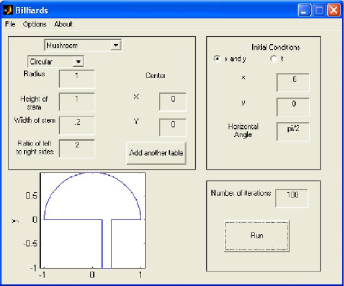
Figure 1: Entering a mushroom table and initial conditions.

3.3 Running the simulation

When the ’run’ button is pressed, Matlab begins the simulation. The program displays the number of iterations completed out of the total number requested. The ’stop’ button discontinues the simulation. The module will not respond to user interactions until the current iteration is completed.

3.4 Analysis

The analysis window displayed in Figure 2 will appear after the simulation is complete. The raw data from the simulation can be exported with the raw data box on the left. This option enables the user to further analyze the calculated data. The desired type of data should be selected from the list box on the left and can either be displayed in the command window or saved by choosing the appropriate radio button. The ’OK’ button on the left exports the data. The ’Pieces hit’ option gives the symbolic dynamics of the initial conditions; the pieces are assigned numbers based on the order of the parametric functions in the piecewise definition of the table.

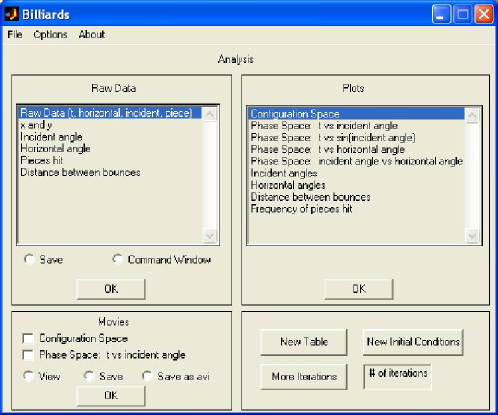
Figure 2: Analysis window for Billiards.

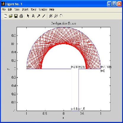
Figure 3: Configuration space for the mushroom with an integrable trajectory depicted.

Specific plots can be generated with the list box on the right. The configuration space (see Figure 3) displays the table and the paths of any trajectories. The phase space plots display Poincaré sections of the billiard system. The variable $t$ gives the location on the boundary at which the point particle collides; it is defined by the parametric equations describing the table. The incident angle $\phi$ gives the direction of the point particle after the collision and is measured relative to the normal of the boundary at the collision point. The horizontal angle $\theta$ gives the direction of the point particle after the collision with respect to the horizontal. Figure 4 shows the phase space of $t$ vs $\sin(\phi)$ for the Bunimovich mushroom. The incident angles, horizontal angles, distance between bounces, and frequency of pieces hit options display histograms of the appropriate data, although it may be desirable to export this data in order to perform additional analysis. The histograms are generated using the Matlab function hist. The plots are displayed by pressing the ’OK’ button on the right side. The billiard table and data can be saved and opened later using the file menu.

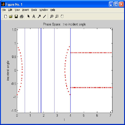
Figure 4: Phase space for the mushroom with an integrable trajectory depicted.

3.5 New initial conditions

The options in the bottom right of the window enable the user to generate additional data. The ’New Table’ button clears all data and resets the program so that a new table can be entered. The ’New Initial Conditions’ button retains all the calculated data, and the user can enter new initial conditions for the current table. More iterations are calculated for the same initial conditions by entering the desired number of additional iterations and pressing the ’More Iterations’ button. The program will continue where the last simulation stopped.

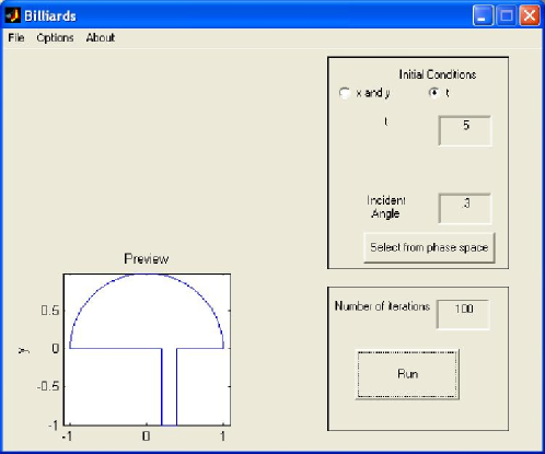
Figure 5: Entering new initial conditions for the mushroom.

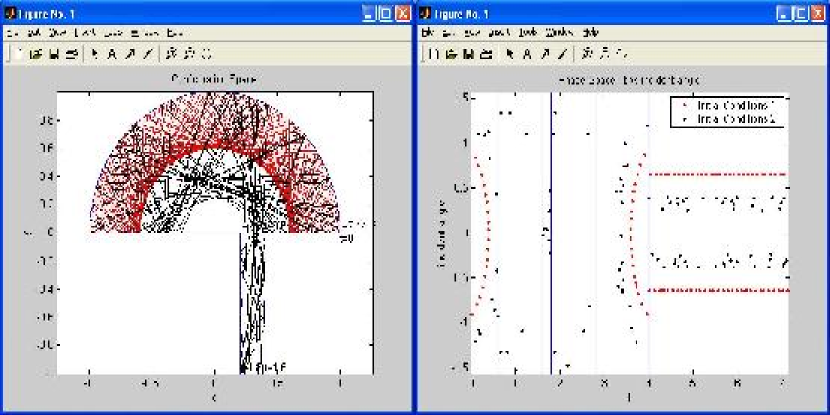
Figure 6: Configuration space and phase space of a mushroom billiard with two initial conditions depicted.

To continue the mushroom example, click on the ’New Initial Conditions’ button. This time, we will enter the initial conditions using the arclength variable $t$. With this method, one specifies a location on the table boundary with $t$ and a direction by specifying the incident angle of the trajectory to the table. One may either type in values for $t$ and the incident angle or select them from phase space. Clicking on the ’Select from phase space’ button will open a plot of phase space with data from all previous initial conditions. Use the cross hairs to select an initial condition, and the corresponding coordinates are entered into the billiard simulator. If more accuracy is desired than is possible with the cross hairs, the zoom tool can be used to magnify a particular portion of phase space. In this case, the coordinates from phase space must be typed into the program. To continue with this guided example, enter the initial conditions shown in Figure 5.

After Matlab’s computations are done, the analysis window is again displayed. The resulting configuration and phase space plots are depicted in Figure 6. Note that the first set of initial conditions specifies a trajectory that remains in the semicircular region of the mushroom. The set of all such trajectories comprise an integrable region of phase space. On the other hand, the second set of initial conditions corresponds to a trajectory that collides with the stem of the mushroom. These trajectories form a chaotic region of phase space. This example shows how circular mushrooms exhibit a divided phase space that contains exactly one integrable region and exactly one chaotic region.[1]

4 Composite Billiard Tables

Composite billiard tables can be constructed by combining multiple simple billiard tables. Such composite tables are necessary, for example, when considering any table in which the boundary cannot be described by one continuous curve. (One composite table, the Sinai billiard, is preprogrammed.) One can implement such tables with the ’Add another table’ button. To illustrate this, consider a composite table consisting of an off-center circle inside an ellipse. First, the ellipse is selected from the ’Pick a table’ pop-up menu. One enters parameters for the lengths of the horizontal and vertical axes. The ’Add another table’ button appears once both parameters are entered. Figure 7 displays the entered ellipse and the ’Add another table’ button.

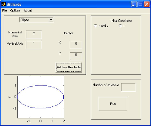
Figure 7: Entered parameters and preview of the ellipse.

The second component of the composite table can now be added. It is entered as normal except that the previous component remains a part of the table. In this example, the circle option is selected from the pop-up menu. The radius is entered as normal. Now we need to move the circle so that the circle and the ellipse are not concentric. This is accomplished by editing the $x$ and $y$ coordinates under the center label. The preview is redrawn once the center of the current component of the table has been moved to the new coordinates. Figure 8 shows the completed composite table. The numbering of the pieces and value of the variable $t$ for each subsequent component of a composite table continue where the previous components left off.

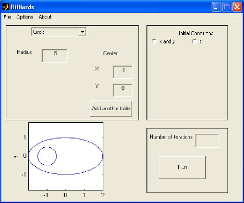
Figure 8: Completed composite table.

5 Billiard Table Maker

The strength of the billiard program lies in its generality, as it can simulate any classical planar billiard system. If one desires to analyze a table that is not preprogrammed, it can be designed using the Billiard Table Maker, which is opened by selecting ’Custom table…’ from the ’Pick a table’ pull-down bar.

As an example, we will use the Billiard Table Maker to create a stadium billiard modified so that one of the straight segments is replaced by a sinusoidal function. We start by creating a vertical line that will form one side of the modified stadium. To do this, click the ’Line’ button. At this point, note that the mouse controls a pair of cross hairs that are used to select the starting and ending points of the line. For this example, $(1,2)$ and then $(1,-2)$ were selected. The program then draws the line segment connecting these two points, as shown in Figure 9.

Figure 9: Line segment drawn with the Billiard Table Maker.

We now wish to add a semicircular region to form the bottom of the modified stadium. Because we are adding a new piece where the previous one ended, we want to use the ’Continue from last endpoint’ feature on the left, which is the default setting. The ’Start at new endpoint’ feature allows one to construct tables that cannot be described with a single boundary curve. Click on the ’Semicircle’ button. Using the cross hairs, select $(-1,-2)$ for the endpoint of the semicircle and select any point above the line connecting the endpoints of the semicircle to designate the inside of the semicircle. The resultant table is shown in Figure 10.

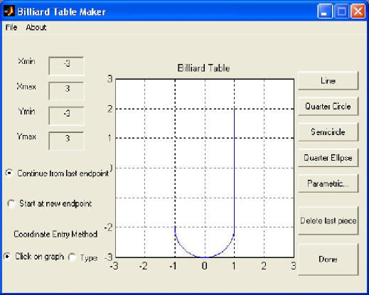
Figure 10: Semicircle added to the endpoint of the previous piece.

The next piece to add is a sinusoid for the left side of the modified stadium. As this is not a basic piece (line segment, quarter circle, semicircle, or quarter ellipse), we must use the ’Parametric…’ push button. With this feature, one can add a piece by entering parametric equations of a curve. Clicking on the push button brings up a window in which one enters $x(t)$, $y(t)$, and lower and upper bounds for $t$. Note that the default value for the lower bound is $0$, but this can be changed to any desired value. The parametric equations for this example and the resultant table are shown in Figure 11. The vertical axis of the window has automatically been scaled to make sure the last piece is shown in the grid. The axis can be edited manually by changing the minimum and maximum values for $x$ and $y$ displayed on the left.

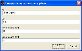
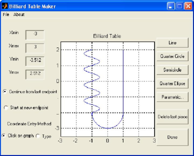
Figure 11: Parametric equations for the sinusoidal piece of the table and the resultant table.

We will now add an upper semicircle to complete the billiard table. To illustrate this feature, select the radio button ’Type’ under ’Coordinate Entry Method.’ This enables the user to accurately specify the coordinates of the input points. Because the program rounds input points, the alternate method of clicking on the graph to select points only allows points with integer coordinates to be selected. Clicking on the ’Semicircle’ push button brings up a window to enter coordinates. The entered coordinates and the final billiard table are shown in Figure 12. Quarter ellipses in which the major and minor axes are parallel to the coordinate axes can also be created in a similar manner by using the ’Quarter Ellipse’ button. One can either save the table now or return to Billiards by clicking on the ’Done’ button.

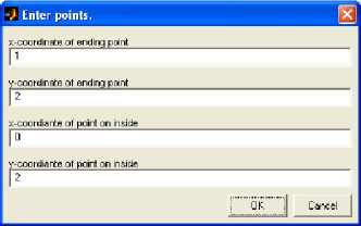
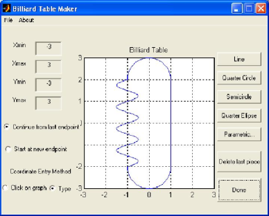
Figure 12: Entering coordinate points for semicircle and completed billiard table.

6 Movies

One can create movies to view an animation of generated billiard data. Controls for doing this are located at the bottom left of the analysis window. Movies of configuration and/or phase space can be created by checking the appropriate boxes. Such movies show one frame for each iteration and highlight the most recently drawn iteration. The frames rate can be modified using the options menu. Movies can only be created for the most recent initial condition and should be used only with a small number of iterations due to memory limitations. By selecting the appropriate radio button, the movie can be viewed in Matlab, saved as a Matlab movie, or saved as an .avi file. For every option, each frame of the animation is first displayed on the screen. After all frames have been rendered, the movie will be displayed or a save dialog box will appear depending on which radio button is selected.

7 Description of Tables

The program stores billiard tables in a cell array. For example, Table 1 shows the table created in the previous section. A table is given by a piecewise function; each row describes a piece of the table. The first and second columns are parametric equations for the $x$ and $y$ coordinates for each piece of the table [$x(t)$ and $y(t)$]. The equations are stored as Matlab inline functions. The third and fourth columns give the bounds for $t$, which is used as the dummy variable for the parametrization. The functions $x(t)$ and $y(t)$ have been scaled to the appropriate expressions so that $t$ also represents the arc length from the starting point of the billiard table to the current point for a given connected component of the billiard. For composite tables, the value of $t$ for each component starts at the same value of $t$ used at the end of the previous component. The final column of the table contains a flag that determines the nature of the piece. For line segments, $1$ is stored in the final column; for circular or elliptical arcs, $2$ is stored in the final column; if the piece is neither a line segment nor one of arcs specified above, then $0$ is stored in the final column. Note, however, that if a piece is entered by typing in parametric equations, then the final column is automatically $0$ regardless of the actual identity of the piece. Circular and elliptical arcs that sweep out arbitrary angles must be entered parametrically. The three different types of pieces are treated differently during the simulation.

Parametric equations that constitute exterior boundaries to the table must be traced in the clockwise direction, whereas interior boundaries must be traced in the counterclockwise sense. For example, the exterior square of the Sinai billiard is oriented clockwise, and the interior circle is oriented counterclockwise. If the wrong direction is used to parameterize the boundary, specifying initial conditions using $t$ and the incident angle will not work properly, as the incident angle will be on the wrong side of the curve.

$x(t)$ $y(t)$ lower bound upper bound flag 1 $2-t$ 0 4 1 cos(-$t$+4) -2+sin(-$t$+4) 4 7.1416 2 .5*sin(2*$\pi$*($t$-7.1416))-1 $t$-9.1416 7.1416 11.1416 0 cos[(-$t$+11.1416)+3.1416] 2+sin[(-$t$+11.1416)+3.1416] 11.1416 14.2832 2

Table 1: Representation of table created in Section 5.

8 Description of Raw Data

The billiard simulator calculates and stores information describing each collision of the point particle with the boundary. For example, consider the simulation of a regular pentagon with side length $1$ and initial location $(0,0)$ with an angle of $2$. Figure 13 shows the configuration space for this simulation; raw data is presented in Table 2.

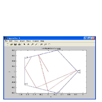
Figure 13: Configuration space of pentagon simulation.

$t$ horizontal angle incident angle piece 3.4205 -1.3717 -0.1150 4.0000 1.2935 0.7434 -0.5133 2.0000 4.9418 -2.6283 -0.1150 5.0000 1.6438 2.0000 0.7434 2.0000 2.6301 1.1416 1.1416 3.0000 3.2091 -0.5133 0.7434 4.0000

Table 2: Data for pentagon simulation.

Each collision with the table is described by a row of data. The location of the point on the boundary that the particle hits is given in the first column as a value of $t$. This value can be converted into $x$ and $y$ coordinates by evaluating the appropriate expressions in the table matrix. The second column gives the horizontal angle $\theta\in[-\pi,\pi]$, which is a measure of the angle of a vector in the direction the particle travels after colliding with the boundary. The quantities $t$ and $\theta$ give, respectively, the position and direction of the point particle immediately after its collision with the boundary. The third column contains the tangential angle $\phi\in[-\pi/2,\pi/2]$, which is the angle between the normal to the position of the boundary the particle hits and the exiting path taken by the particle. Negative angles indicate the exiting path is clockwise from the normal, whereas positive angles indicate that the exiting path is counterclockwise from the normal. The fourth column gives the piece the particle hits. The sequence of such pieces encodes a symbolic dynamics for the given trajectory. Sets of data for each initial condition are stored by the program in a cell array called ’data.’

9 Calculation of iterations

The program runs iteratively in its simulation of classical billiards. Given the position and direction of the previous collision, the program calculates the position and direction of the point particle after its subsequent collision with the boundary. To find the location of the next collision, the program searches for an intersection between the line that describes the path of the point particle and each of the table’s parametric pieces. Given all such intersections, the point with the minimum distance traveled is the next point of intersection. To find the direction in which the point particle travels following the collision, the normal angle to the boundary is computed from the derivatives of the equations of the table at the point of intersection. Addition and subtraction of angles is used to calculate the exit angle from the normal angle and the entrance angle:

$$\theta_{n} =2\arctan\Big{(}\frac{dy}{dt}\Big{/}\frac{dx}{dt}\Big{)}\Big{|}_{t_{n}}-\theta_{n-1}\,,$$

$$\phi_{n} =\arctan\Big{(}\frac{dy}{dt}\Big{/}\frac{dx}{dt}\Big{)}\Big{|}_{t_{n}}-\theta_{n-1}+\pi/2\,,$$ (1)

where $\theta_{n}$ represents the angle with respect to the horizontal of the $n$th iteration, $\phi_{n}$ represents the incident angle of the $n$th iteration, $y(t)$ and $x(t)$ are the parametric equations of the boundary, and $t_{n}$ is the value of $t$ that gives the location of the $n$th intersection with the boundary. In Matlab, equation (1) is implemented using the ‘arctan2’ function to ensure that one obtains the correct quadrant for the angle. Additionally, note that $\phi_{n-1}$ does not appear in the right-hand-side of (1), as this angle is used only for phase space plots and is not involved in the calculation of angles in subsequent iterations.

9.1 Corners

Special consideration must be employed if the point particle collides with a corner of the billiard table, as such points correspond to singular points of the billiard (Poincaré) map obtained from examining only the collisions (and not the straight paths between them) of the vector field describing the billiard system.[4] This occurs when the point particle’s path reaches a point where two pieces of the table join abruptly (with discontinuous first derivative with respect to arc length). In the present numerical implementation, whenever the point particle collides with the boundary at a point where $t$ is within $10^{-8}$ of the beginning or end of a piece, it is considered to have hit a corner. In order to numerically compute the angle with which the point particle leaves the collision, the tangential angles of the two pieces of the table are averaged. The point particle subsequently bounces off a boundary oriented at this angle as if the collision were normal. (When studying billiard systems using this program, one needs to be careful if a trajectory hits the boundary too close to a corner.)

10 Precision

Errors due to round-off can grow quickly with our billiard simulations, as frequently occurs for repetitive numerical approximations. The rate that the errors compound depends fundamentally on the geometry of the billiard table. For certain billiard tables, the error is negligible for a very large number of iterations. For others, this is not the case.

Two examples are presented to demonstrate how the accuracy of the simulation depends on the particular table. In the circular billiard with unit radius, we examined the trajectory starting at $(.5,0)$ with an initial horizontal direction. The maximum error in the incident angle after $10,000$ iterations was only $1.1213\times 10^{-13}$.

Consider, however, a billiard table consisting of two circles of unit radius with respective centers at $(1.5,0)$ and $(-1.5,0)$. The initial conditions were set to the origin with a horizontal angle. The point particle was then calculated to escape the two circles due to round-off error after $10$ iterations. This extreme example of a numerically unstable periodic orbit demonstrates that one must be cautious when using the program.

11 Known Errors

The current program is not yet reliable for tables that contain pieces that are not line segments or elliptical arcs. The program will work properly until it fails to find where a trajectory intersects a complex curve. This problem is due to an inability of the program to reliably find a zero of a given function on a given interval.

12 Additional Features to be Implemented

A useful analytical tool would entail the creation of a Markov partition of phase space.[2] For each point in phase space, the piece against which the point particle will collide on the next iteration will be determined. This will create a Markov partition by dividing phase space so that every point in the same region will collide with the same piece on the next iteration. This will be visually implemented by coloring phase space. The partition will allow one to easily view the symbolic dynamics for the first several iterations associated with any initial condition.

One can implement a Markov partition by finding the critical angles that cause the next collision of the point particle to collide with a different piece. The vertical segment of phase space that corresponds to this location can then be colored based on which piece will next be hit. This process will then continue for the entire boundary of the billiard table; all of these vertical segments are then joined to form the Markov partition.

If the regions of phase space described above can be found, the Markov partition can be used to speed up the billiard simulator considerably. For each iteration, the program currently must check all pieces of the table to find the proper intersection. This process is very costly, as a floating point root finder is used each time to find all possible intersections between the point particle’s path and the table. With the implementation of a Markov partition, the program will be able to determine which segment the particle subsequently hits instead of searching for the right piece. The progrom will no longer spend time finding irrelevant roots, which will improve the speed and efficiency of the billiard simulator substantially.

Future versions of the program can also include computations of important quantities such as Lyapunov exponents. In the long run, we would ultimately like to expand the program to simulate quantum billiards as well as classical ones. Phenomena such as scarring would then be especially easy to study.

13 Conclusions

We created a GUI Matlab module that simulates classical billiards. It provides a useful research and teaching tool for scientists interested in these dynamical systems. This module’s simulations can be used not only to produce accurate phase space and Poincaré section plots for scientific publications but also to gain considerable mathematical and physical insight.

References

- [1] Leonid A. Bunimovich. Mushrooms and other billiards with divided phase space. Chaos, 2(4):802–808, December 2001.
- [2] Predrag Cvitanović, Roberto Artuso, Per Dahlqvist, Ronnie Mainieri, Gregor Tanner, Gregor Tanner, Gábor Vattay, Niall Whelan, and Andreas Wirzba. Classical and Quantum Chaos, volume Version 10. Niels Bohr Institute, July 2003. www.nbi.dk/ChaosBook/.
- [3] Martin C. Gutzwiller. Chaos in Classical and Quantum Mechanics. Number 1 in Interdisciplinary Applied Mathematics. Springer-Verlag, New York, NY, 1990.
- [4] Anatole Katok and Boris Hasselblatt. Introduction to the Modern Theory of Dynamical Systems. Cambridge University Press, New York, NY, 1995.
- [5] H. J. Korsch and H.-J. Jodl. Chaos: A Program Collection for the PC. Springer-Verlag, 2nd edition, 1999.