Relation between shear parameter and Reynolds number in statistically stationary turbulent shear flows

Abstract

Studies of the relation between the shear parameter $S^{*}$ and the Reynolds number $Re$ are presented for a nearly homogeneous and statistically stationary turbulent shear flow. The parametric investigations are in line with a generalized perspective on the return to local isotropy in shear flows that was outlined recently [Schumacher, Sreenivasan and Yeung, Phys. Fluids 15, 84 (2003)]. Therefore, two parameters, the constant shear rate $S$ and the level of initial turbulent fluctuations as prescribed by an energy injection rate $\epsilon_{in}$, are varied systematically. The investigations suggest that the shear parameter levels off for larger Reynolds numbers which is supported by dimensional arguments. It is found that the skewness of the transverse derivative shows a different decay behavior with respect to Reynolds number when the sequence of simulation runs follows different pathways across the two-parameter plane. The study can shed new light on different interpretations of the decay of odd order moments in high-Reynolds number experiments.

I Introduction

Homogeneous shear turbulence can be considered as the first non-trivial extension of homogeneous, locally isotropic turbulence. It is a flow that is thought as a bridge between the strongly idealized homogeneous isotropic turbulence and more realistic turbulent shear flows such as channel flows pope2000 . A constant mean shear rate $S$ is present which is a large-scale source of anisotropy and the question that immediately arises is how the statistical properties at the smallest scales of the turbulent flow are affected by its presence. After the pioneering work of Lumley lumley1967 in which he predicted by dimensional arguments a rather rapid decay of such anisotropy, namely with $\sim R_{\lambda}^{-1}$, this particular flow came under renewed interest in the last decade. Several systematic measurements in simple shear flows gargwarhaft1998 ; ferchichitavoularis2000 ; shenwarhaft2000 ; staicuvandewater2003 and in atmospheric boundary layers for the largest accessible Taylor microscale Reynolds numbers of $R_{\lambda}\sim 10^{4}$ were presented.kuriensreenivasan2000 All experiments detected systematic deviations from Kolmogorov’s concept of local isotropy. kolmogorov1941 The decay of odd order normalized transverse derivative moments with respect to Taylor microscale Reynolds number occurs with a larger exponent than -1 and the co-spectrum of the shear stress deviates from the classical -7/3 law.kuriensreenivasan2000 For moderate Reynolds numbers, such a persistence in the decay of odd order moments was also found within direct numerical simulations (DNS) and its connection to coherent structures and intermittency corrections could be addressed.pumir1996 ; schumachereckhardt2000 ; schumacher2001 ; gualtierietal2002 ; ishiharaetal2002

Recently, the record of experimental and DNS data on homogeneous and nearly homogeneous shear flows was collected and discussed anew from a generalized perspective by taking into account the role of small-scale intermittency and mean shear.schumacheretal2003 It was found that the operating points of all those experiments are scattered in a two-parameter plane which is spanned by the Reynolds number $Re$ and the shear parameter $S^{*}$. Different experiments followed different pathways across such plane causing, e.g., variations in the decay behavior of odd order moments when simply projected onto the Reynolds number axis as it is done usually when the issue of isotropy is discussed. This was identified as one possible reason for different interpretations of the data in terms of the return to local isotropy for higher Reynolds numbers.

One outcome of Ref. 14 is the necessity for more systematic numerical experiments which will be presented in the following. Here, two system parameters that determine the homogeneous shear flow will be varied: the constant shear rate, $S$, and an energy injection rate, $\epsilon_{in}$, that prescribes the amount of initially isotropic turbulent fluctuations. The latter parameter can also be thought of as a substitute for active or passive grids that are often placed in wind tunnel experiments before the working fluid enters the shear straightener (see e.g. Refs. 4 to 6 and the sketch in Fig. 1). Such additional device (which is optional, but frequently used) increases the turbulent fluctuations and thus the Reynolds number while operating with the same mean shear rate $S$. Beside this main motivation coming from the experiments in nearly homogeneous shear flows, it allows here for reaching a stable turbulent regime for small shear rates. Consequently, the numerical experiments will give us hints on the following functional dependencies

$$Re = F_{1}(\nu,S,\epsilon_{in})\,,$$ (1)

$$S^{*} = F_{2}(\nu,S,\epsilon_{in})\,,$$ (2)

and would therefore allow for a more systematic study of the deviations from local isotropy, e.g. how transverse derivative moments decay along particular pathways across the two-parameter plane. We can simplify the functional dependencies in relations (1) and (2) by keeping the kinematic viscosity $\nu$ constant throughout the study.

Figure 1: Sketch of a typical experimental situation in a simple shear flow and its relation to the present investigation. A shear straightener sets up a mean flow with a shear rate $S$ and an active or passive grid produces additional turbulent fluctuations. The turbulence is decaying along the downstream direction. The small volume would be the one we model within the DNS.

Numerical models for homogeneous shear turbulence can be divided into three different groups. The first one uses finite difference methods with shear periodic boundary conditions on the grid in physical space.gerzetal1989 The other two approaches use pseudospectral techniques with periodic boundary conditions. Rogallo suggested a time-dependent coordinate transformation for the inclusion of constant shear in such a simulation of turbulence. rogallo1981 ; rogersmoin1986 The consequence is that the numerical grid gets steadily skewed and has to be remeshed after time $t=2/S$. In this method, it was hard to reach a stationary turbulent state, the integral length scale grows exponentially in time until the order of the box length is reached. Statistical investigations that continued afterwards had to be run for very long time intervals due to large fluctuations of energy or enstrophy. pumir1996 ; gualtierietal2002 ; yakhot2003 In Ref. 9 integrations up to $St\sim 10^{3}$ were performed. For very large $S$ aliasing errors were reported.leeetal1990 A method to overcome some of the problems was suggested recently.schumachereckhardt2000 The method avoids the remeshing procedure. A statistically stationary state with smaller fluctuations of energy and enstrophy can be attained by an appropriate volume forcing in combination with free-slip boundary conditions. The boundary conditions will cause small deviations from transverse homogeneity, so strictly speaking our system is a nearly homogeneous shear flow, as it is the case for the measurements.

The outline of the manuscript is as follows. In the next section, we present in brief the numerical model and the volume forcing schemes which are related to both outer parameters, $S$ and $\epsilon_{in}$. In section III we conduct detailed studies of the statistical stationarity and point to differences in comparison with the classical remeshing approach. Afterwards, we are going to discuss the relation between shear parameter and Reynolds number. Predictions that are made on the basis of dimensional arguments will be compared with numerical findings. Based on these results, the behavior of derivative moments with respect to Reynolds number and shear parameter will be studied. Finally, a summary and an outlook are given.

II Numerical model

II.1 Equations and boundary conditions

With length scales measured in units of the box width $L_{y}$, and time scales in units of the eddy turnover time $L_{y}/v_{rms}$, the dimensionless form of the equations for an incompressible Navier–Stokes fluid become

$$\frac{\partial{\bf u}}{\partial t}+({\bf u}\cdot{\bf\nabla}){\bf u} = -{\bf\nabla}p+\frac{1}{Re}{\bf\nabla}^{2}{\bf u}+{\bf F}\;,$$ (3)

$${\bf\nabla}\cdot{\bf u} = 0\;,$$ (4)

where $p({\bf x},t)$ is the pressure, ${\bf u}({\bf x},t)$ the velocity field. The large scale Reynolds number is then

$$Re=\frac{v_{rms}L_{y}}{\nu}\,.$$ (5)

The velocity components are decomposed in a mean fraction and a fluctuating turbulent part, $u_{i}=\langle u_{i}\rangle+v_{i}$ for $i=x,y$ and $z$, the so-called Reynolds decomposition. The mean flow profiles are given for the homogeneous shear flow by

$$\langle u_{x}\rangle_{A,T}=Sy,\,\,\,\langle u_{y}\rangle_{A,T}=\langle u_{z}\rangle_{A,T}=0,$$ (6)

where $x$ are streamwise (or downstream), $y$ shear (or wall-normal), and $z$ spanwise directions, respectively. Statistical averages are denoted by parentheses for the following and indices indicate whether a time average, $\langle\cdot\rangle_{T}$, a volume average, $\langle\cdot\rangle_{V}$, an average over $x-z$ planes at fixed y, $\langle\cdot\rangle_{A}$, or combinations of them are taken. Consequently, the root mean square velocity reads $v_{rms}=\sqrt{\langle{\bf v}^{2}\rangle_{V,T}}$ and the dimensionless shear parameter becomes

$$S^{*}=\frac{Sv^{2}_{rms}}{\epsilon}\,,$$ (7)

with the energy dissipation rate $\epsilon=\langle\epsilon({\bf x},t)\rangle_{V,T}$ and $\epsilon({\bf x},t)=(\nu/2)\sum_{i,j}(\partial_{j}v_{i}({\bf x},t)+\partial_{i}v_{j}({\bf x},t))^{2}$.

The pseudospectral method is applied. The equations are integrated by a second order predictor-corrector scheme where the time stepping satisfies the Courant-Friedrichs-Levy criterion. The Courant number was always below 1/2. The dissipative term was included as an integrating factor $\exp(-\nu k^{2}t)$ for every mode ${\bf u}_{\bf k}(t)$. De-aliasing is done by a combination of 2/3-rule truncation and phase-shifting rogallo1981 . As a criterion for sufficient spectral resolution $k_{max}\eta>1$ is used pope2000 with Kolmogorov length scale $\eta=(\nu^{3}/\epsilon)^{1/4}$ and $k_{max}=\sqrt{2}N/3$. The aspect ratio $L_{x}:L_{y}:L_{z}=2\pi:\pi:2\pi$ was resolved with $N\times(N/2+1)\times N$ grid points where $N=256$ and 512, respectively .

We take periodic boundary conditions in streamwise and spanwise directions, respectively. In the shear direction, free-slip boundary conditions are applied,

$$u_{y}=0,\;\;\text{and}\;\;\frac{\partial u_{x}}{\partial y}=\frac{\partial u_{z}}{\partial y}=0.$$ (8)

The free-slip boundary conditions will cause slight deviations from the transverse homogeneity, an effect which decreases with growing Reynolds number eckhardtschumacher01 . In contrast to the no-slip case, no energy is transfered into the flow via the free-slip boundaries and thus an additional volume forcing ${\bf F}$ has to be applied (cf. eq. (3)) in order to sustain turbulence.

II.2 Forcing scheme

A compact formulation of the Navier-Stokes equations in Fourier space for our problem is given by

$$\frac{\partial u_{i{\bf k}}}{\partial t} = N_{i{\bf k}}(u_{j{\bf q}},t;Re)+F_{i{\bf k}}(t)\;,$$ (9)

where $N_{i{\bf k}}$ contains all nonlinear mode coupling contributions and the dissipative part, $-Re^{-1}k^{2}u_{i{\bf k}}(t)$. In the following we will combine two kinds of forcing, a volume forcing that sustains the linear mean flow profile which will be referred to as shear forcing and a homogeneous forcing that mimics the injection of additional fluctuations by the grid which will be referred to as grid forcing.

A handful of Fourier modes is driven now in order to give an almost linear profile for $\langle u_{x}\rangle_{A,T}$, i.e. the forcing is with respect to the streamwise velocity component only. The driven modes are for the wave vectors ${\bf k}^{\prime}=(0,2n+1,0)$ for $n=0$ to 5. They form the almost linear mean profile,

$$\langle u_{x}\rangle_{A,T}(y)=\frac{2\alpha}{\pi}\left(y-\frac{\pi}{2}\right)\approx-\frac{8\alpha}{\pi^{2}}\sum^{5}_{n=0}\frac{\cos[(2n+1)y]}{(2n+1)^{2}}\,,$$ (10)

for $y\in[0,\pi]$. This results in a mean shear rate $S=2\alpha/\pi$. The shear forcing is chosen in such a way that just these modes (which have real parts only for symmetry reasons) are held fixed to the amplitude values as given by Eq. (10), i.e.

$$\frac{\partial u_{x{\bf k}^{\prime}}}{\partial t}=0\;\;\;\;\Leftrightarrow\;\;\;\;F^{(s)}_{x{\bf k}^{\prime}}(t)=-N_{x{\bf k}^{\prime}}(u_{j{\bf q}},t;Re)\;.$$ (11)

These coefficients are set at the begining and do not violate the boundary conditions and the divergence-zero condition because the driven modes $u_{x{\bf k}^{\prime}}(t)$ are functions of $k_{y}^{\prime}$ only. The particular kind of forcing in the Fourier space might be nonanalytic in the real space and will vary in space and time.

Second, the grid forcing at small wavenumbers is applied that injects a certain amount of energy per time unit into the flow given by the rate $\epsilon_{in}$, grossmannlohse1994

$${\bf F}^{(g)}_{{\bf k}^{\prime\prime}}(t)=\epsilon_{in}\frac{{\bf u}_{\bf k}(t)}{\sum_{{\bf k}^{\prime\prime}\in K}|{\bf u}_{{\bf k}^{\prime\prime}}(t)|^{2}}\,\delta_{{\bf k,k}^{\prime\prime}}\;.$$ (12)

Consequently, it would follow

$$\sum_{\bf k}{\bf u}^{*}_{\bf k}(t)\cdot{\bf F}^{(g)}_{\bf k}(t)=\epsilon_{in}\equiv\epsilon\,,$$ (13)

for the statistically stationary balance of the turbulent kinetic energy when $S\equiv 0$. The wavenumbers of the set $K$ do not coincide with the ones for the shear forcing, but are also small.

III Statistical stationarity

III.1 Difference to the remeshing method

The Reynolds decomposition of eqns. (3) and (4) for all fields results in

$$\langle u_{j}\rangle\partial_{j}\langle u_{i}\rangle = -\partial_{i}\langle p\rangle+\frac{1}{Re}\partial_{j}^{2}\langle u_{i}\rangle+\langle F_{i}\rangle-\partial_{j}\langle v_{i}v_{j}\rangle\;,$$ (14)

where we considered already the time independence of the mean profile. At this point, a difference to the case with remeshing becomes obvious. All terms of the equation will be zero independently of each other due to exact homogeneity for the latter case. The violation of the transverse homogeneity will cause relics in the Reynolds balance for the present model and results in

$$0=\langle F_{x}^{(s)}\rangle_{A,T}-\partial_{y}\langle v_{x}v_{y}\rangle_{A,T}\;.$$ (15)

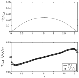
Figure 2: Upper panel: Reynolds shear stress $-\langle v_{x}v_{y}\rangle_{A,T}$ as a function of $y$. Average was taken with respect to time and over $x-z$ planes at fixed $y$. Lower panel: Verification of relation (15). It can be seen that $\langle F_{x}^{(s)}\rangle_{A,T}$ and $\partial_{y}\langle v_{x}v_{y}\rangle_{A,T}$ collapse for almost all $y$.

Figure 2 illustrates this behavior. We show the vertical profile of the shear stress, $\langle v_{x}v_{y}\rangle_{A,T}$ (upper panel) and verify that Eq. (15) is satisfied to a good approximation except very close to the boundaries (lower panel). The upper panel shows also that our system becomes nearly homogeneous only with respect to the transverse direction. To conclude, there is a difference between both methods for the large scale balance. The question is now: how are small-scale statistical properties of the fluctuating quantities affected in the present approach? As demonstrated in Refs. 10 and 11 small scale statistical properties such as Reynolds stress magnitudes or higher order normalized moments of the transverse derivative and spanwise vorticity, respectively, agree with previous homogeneous shear flow simulations rogersmoin1986 ; pumir1996 and experiments for the lowest Reynolds numbers shenwarhaft2000 .

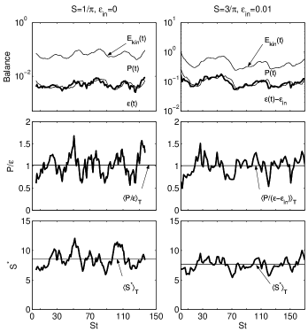
Figure 3: Statistical stationarity of the shear flow. Left column is for run IV, the right column is for run IIc (see Tab.1). Upper panels: Temporal evolution of turbulent kinetic energy $E_{kin}(t)$, energy dissipation rate $\epsilon(t)$ (thin solid line), and production of turbulent kinetic energy $P(t)$ (thick solid line). Mid panels: Temporal evolution of the ratio $P(t)/\epsilon(t)$. The thin solid line is the temporal mean of the data and very close to one. Lower panels show the temporal variation of the shear parameter $S^{*}$. Temporal means are again indicated by thin solid lines.

The forcing keeps the flow in a statistically stationary state with moderate fluctuations of the kinetic energy and enstrophy, respectively (see Ref. 11 for a more detailed investigation). In order to demonstrate this property of the current numerical scheme, we show time series of the turbulent kinetic energy, $E_{kin}(t)=q^{2}(t)/2=\langle{\bf v}^{2}\rangle_{V}/2$, the production of turbulent kinetic energy, $P(t)=-\langle v_{x}v_{y}\rangle_{V}S$, and the energy dissipation rate, $\epsilon(t)=\nu\langle(\partial_{i}v_{j})^{2}\rangle_{V}$ for two runs in Fig. 3 (run IIc and IV of Tab. 1). The fluctuations of the kinetic energy are by about a factor of 2 smaller than those reported in the long-time remeshing runs.pumir1996 ; gualtierietal2002 With $\sigma_{E}=\sqrt{\langle(E_{kin}(t)-\langle E_{kin}\rangle_{T})^{2}\rangle_{T}}$ we get $\sigma_{E}/\langle E_{kin}\rangle_{T}=24\%$ for run IV and 33% for run IIc. This ratio decreases even further for runs Ia to Ie. The resulting global energy balance for the fluctuating part is then

$$\partial_{t}\frac{q^{2}}{2} \approx -\epsilon(t)+P(t)+\epsilon_{in}\,.$$ (16)

It was verified that contributions from shear driving are subdominant as well as the transverse flux contributions from third order terms arising in the balance. The reduced fluctuations of the kinetic energy might be caused due to the free-slip boundaries. As mentioned above, small boundary layers do form that cause slight transverse fluxes into the bulk.hill2001 ; casciolaetal2003

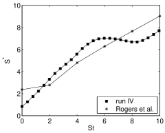
Figure 4: Temporal evolution of the dimensionless shear parameter in the initial phase of the simulation for run IV. The run started with isotropic turbulence decaying with a $k^{-5/3}$ spectral law and was asserted to the constant shear with rate $S$. For comparison we added initial data from Rogers et al. rogersetal86a (run C128V).

As can be seen in Fig. 3, the ratio of $P/\epsilon$ varies in time, but its temporal mean is almost exactly unity and

$$\langle P(t)\rangle_{T}=\langle\epsilon(t)\rangle_{T}-\epsilon_{in}\,,$$ (17)

holds. We note that this property differs from the remeshing simulations where the ratio $P/\epsilon$ is constant but larger unity. Quantities such as the turbulent kinetic energy will grow then exponentially with time which is a consequence of (16), i.e. $q^{2}(t)\sim\exp[(P/\epsilon-1)t]$. One might conclude that the violations of the transverse homogeneity cause this ratio to vary around unit value and thus to assure statistical stationarity. This point should not be mixed with the exclusion of statistical stationarity and downstream homogeneity which is relevant in experiments harrisetal1977 ; tavoularis1985 but not in DNS.

It is interesting to take a closer look at the initial phase of the evolution. In Fig. 4 we plotted the initial evolution of the shear parameter $S^{*}$ and for comparison we added DNS data by Rogers et al. rogersetal86a . Both simulations show that for the initial phase an (almost) linear growth can be detected. It clearly illustrates the non-normal amplification mechanism acting on the isotropic turbulent “background”. The streamwise velocity fluctuations grow due to the lift-up of streamwise streaks, but will leave the energy dissipation rate which is dominant at small scales close to its initial magnitude for a while. In Fig. 5 we show the streamwise turbulent velocity at two instants, an initial snapshot (upper panel) where the fluctuations are still isotropic and a later snapshot (lower panel) where streamwise streaks have formed. A more detailed analysis of the regeneration cycle of these streamwise streaks and vortices waleffe1997 in a shear flow with free-slip boundaries was discussed in Ref. 28 and was found to agree qualitatively with other shear flows.

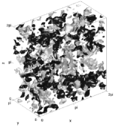
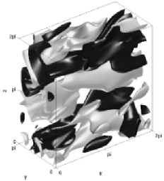
Figure 5: Isosurface plots of the streamwise turbulent velocity for the initial phase of run IV. Level sets with opposite sign are shown in each picture (grey is positive and black is negative). Upper panel: St=0.4. Lower panel: St=9.6.

III.2 Integral scale

In Fig. 6 we show the integral length scale which is defined as pope2000

$$L_{11}(t)=\frac{\pi}{2\langle v_{x}^{2}\rangle}\,\int_{0}^{\infty}\,\frac{E(k,t)}{k}\,dk\,,$$ (18)

with the energy spectrum, $E(k,t)$. In comparison to the simulations that use the remeshing method of Rogallo, it can be seen that $L_{11}(t)$ remains well below the box width for our method and does not grow exponentially in time. It could be shown recently that strong fluctuations of the kinetic energy and the enstrophy, respectively, are related to $L_{11}(t)$ reaching the size of the box length yakhot2003 . The present studies give $L_{11}(t)$ at about 33% of $L_{y}=\pi$ and are smaller as the reported 72% to 80% of $L=2\pi$.pumir1996

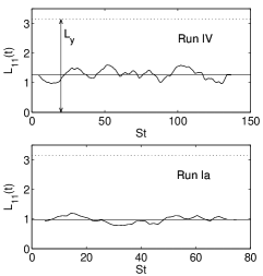
Figure 6: Temporal evolution of the integral length scale $L_{11}(t)$. For comparison, the width of the simulation domain in shear direction $y$ is indicated by the vertical double-headed arrow. The temporal average of $L_{11}(t)$ is plotted as a solid line. Data are for run IV (upper panel) and run Ia (lower panel).

IV Investigations in the two-parameter plane

IV.1 Estimates for the behavior of $S^{*}$ versus $Re$

We turn now to investigations in the parameter plane that is spanned by the two essential dimensionless parameters in a homogeneous shear flow, the shear parameter $S^{*}$ and the Reynolds number $Re$. Every point $(S^{*},Re)$ in this plane will be denoted as an operating point of the particular simulation or measurement, it will drift across the plane for the non-stationary case. As was demonstrated in Ref. 14, the collected data were rather scattered over such a plane. Two limiting regimes for the homogeneous shear flow could be identified. One is the large shear limit which will approach the (linear) rapid distortion case for $S\to\infty$. A condition for the large shear case follows from starting with $|v_{i}\partial\langle u_{j}\rangle/\partial x_{i}|\gg|v_{i}\partial v_{j}/\partial x_{i}|$, and it is given by

$$S^{*}Re^{-1/2}\gg 1\,,$$ (19)

in terms of the large scale Reynolds number $Re$. The second case is the local isotropy limit with the condition of sufficient separation of large and small time scales $S\tau_{\eta}\ll 1$. $\tau_{\eta}=\sqrt{\nu/\epsilon}$ is the Kolmogorov time and it follows

$$S^{*}Re^{-1/2}\ll 1\,.$$ (20)

The idea is to identify a more systematic dependence $S^{*}(Re)$ in the plane, similar to a phase diagram in thermodynamics. It is clear from the beginning that the range of parameters that we can cover with the DNS experiments will be limited, but at least in a certain range we can conduct systematic studies.

Before doing so, we give simple arguments of which functional dependencies (1) and (2) might appear. Dissipation of energy is due to shear effects and due to grid forcing and thus we can set the following relation

$$\epsilon=C_{1}\nu\frac{v_{rms}^{2}}{L_{y}^{2}}+C_{2}\frac{v_{rms}^{3}}{L_{y}}\,,$$ (21)

where $C_{1}$ and $C_{2}$ are dimensionless constants. The two terms on the r.h.s. of (21) model the crossover of the energy dissipation rate from a weakly turbulent state to fully developed turbulence which is present for moderate Reynolds numbers.doeringetal2003 While $\nu v_{rms}^{2}/L_{y}^{2}$ determines the dissipation at smaller Reynolds numbers, the term $v_{rms}^{3}/L_{y}$ takes over for larger Reynolds numbers (for more details see also Ref. 30). The root mean square velocity will be determined by both large scale driving mechanisms and thus

$$v_{rms}=C_{3}\left(L_{y}\epsilon_{in}+C_{4}L_{y}^{3}S^{3}\right)^{1/3}\,,$$ (22)

can be taken by dimensional arguments with yet unknown dimensionless constants $C_{3}$ and $C_{4}$, respectively. Equations (21) and (22) are inserted into the relations for the Reynolds number (5) and the shear parameter (7), respectively. For both parameters follow functions of $S$ and $\epsilon_{in}$ in the presence of constants $\nu$ and $L_{y}$ (cf. Eqns. (1) and (2))

$$S^{*} = \frac{L_{y}^{2}S}{C_{1}\nu+C_{2}C_{3}L_{y}\left(L_{y}\epsilon_{in}+C_{4}L_{y}^{3}S^{3}\right)^{1/3}}\,,$$ (23)

$$Re = \frac{C_{3}L_{y}\left(L_{y}\epsilon_{in}+C_{4}L_{y}^{3}S^{3}\right)^{1/3}}{\nu}\,.$$ (24)

One point becomes obvious immediately: there seems to be a variety of pathways to explore the $S^{*}$–$Re$ plane and the operating points can be scattered over a large fraction. In fact, that is what the collected data points showed. schumacheretal2003

For simplicity, we study the behavior along curves $S$=const and $\epsilon_{in}$=const. The Reynolds number grows to infinity for both cases because one of the sources for an increase of turbulent fluctuations is always present. It reduces to

$$Re_{0}=\frac{C_{3}L_{y}^{4/3}\epsilon_{in}^{1/3}}{\nu}\,,$$ (25)

for turbulence without shear and marks the origin of curves $S^{*}(Re)$ in the plane (cf. relations (19) and (20)). We get the following limits for the shear parameter,

$$\lim_{S=const,\epsilon_{in}\to\infty}S^{*}=0\,,$$ (26)

$$\lim_{\epsilon_{in}=const,S\to\infty}S^{*}=S_{\infty}^{*}=\frac{1}{C_{2}C_{3}C_{4}^{1/3}}\,.$$ (27)

In limit (26) we observe that the shear parameter goes to zero with a power ${\cal O}(\epsilon_{in}^{-1/3})$. Physically, this means that the grid driving becomes more and more important while shear effects decrease, i.e. the system approaches the isotropic limit $S^{*}(Re-Re_{0})^{-1/2}\ll 1$, which is the case to a good approximation in grid turbulence. schumacheretal2003 On the other hand, when keeping $\epsilon_{in}$ fixed but increasing external shear rate $S$, the estimate yields a non-zero constant value if there is no further Reynolds number dependence hidden in the four prefactors $C_{i}$. This means that for a statistically stationary and nearly homogeneous system an asymptotic value of $S^{*}$ is found.

IV.2 Simulation results

The outlined estimates are tested by numerical experiments. In Table I, the different parameter sets and the quantities are summarized that are necessary for the calculation of $S^{*}$ and $Re$. The DNS runs are ordered in three different series, No. I varies along the isoline $(S=const,\epsilon_{in})$, while series II and III run along the iso-parameter line $(S,\epsilon_{in}=const.)$. Such investigation becomes rather expensive because every single data point in the parameter plane is one long-time DNS run for a statistically stationary shear flow.

Run No.	$S$	$\epsilon_{in}$	$v_{rms}$	$\epsilon$	$Re$	$S^{*}$	$k_{max}\eta$	$\nu$	$N$
Ia	$1/\pi$	0.010	0.47	0.017	444	4.2	4.64	1/300	256
Ib	$1/\pi$	0.025	0.55	0.032	520	3.0	3.96	1/300	256
Ic	$1/\pi$	0.040	0.66	0.051	622	2.7	3.52	1/300	256
Id	$1/\pi$	0.055	0.67	0.063	629	2.2	3.34	1/300	256
Ie	$1/\pi$	0.100	0.86	0.114	810	2.1	2.88	1/300	256
IIa	0	0.010	0.34	0.010	325	0.0	5.29	1/300	256
IIb (=Ia)	$1/\pi$	0.010	0.47	0.017	444	4.2	4.64	1/300	256
IIc	$3/\pi$	0.010	0.94	0.111	891	7.7	2.90	1/300	256
IId	$6/\pi$	0.010	1.49	0.480	1404	8.8	2.01	1/300	256
IIe	$8/\pi$	0.010	3.39	2.998	3197	9.8	2.54	1/300	512
IIIa	0	0.025	0.48	0.025	457	0.0	4.21	1/300	256
IIIb (=Ib)	$1/\pi$	0.025	0.55	0.032	520	3.0	3.96	1/300	256
IIIc	$6/\pi$	0.025	1.31	0.393	1235	8.4	2.11	1/300	256
IV	$1/\pi$	0	0.36	0.005	452	8.2	5.07	1/400	256

Table 1: Parameters of the numerical experiments. For convinience we listed the runs in three series indicating different pathways in the parameter plane. Run IV was an additional long-time run for investigations on statistical stationarity.

In Fig. 7, we have collected the operating points $(S^{*},Re)$ of the runs and added the error bars. The inset illustrates the corresponding variations in terms of the outer parameters. We fitted the dimensional estimates to the whole set of data points. The dashed and the dotted lines are the fit results of (23) and (24) to series I, II, and III. The additional lines illustrate how points $(S,\epsilon_{in})$ are mapped to $(S^{*},Re)$ with the fitted constants. It can be seen that the lines display the trends of the data points quite well, but do not match perfectly with the data points. Clearly, the data base is rather sparse such that for a multi-dimensional fit problems can arise. Second, we do observe that the error bars grow in magnitude for the larger shear rates when the fluctuations of large scale velocity tend to grow because the effect of non-normal streak lift-up gets more pronounced.

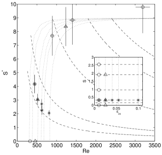
Figure 7: Operating points of statistically stationary homogeneous shear flow simulations in the $Re$–$S^{*}$ parameter plane when iso-parameter lines were followed as indicated in the inset. Asterisks are data points of series I, open circles of series II, and open triangles of series III. The error bars ($\pm\sigma/2$) are given in the panel. They follow from $\sigma_{S^{*}}=S^{*}(2\sigma_{v_{rms}}/v_{rms}+\sigma_{\epsilon}/\epsilon)$ and $\sigma_{Re}=Re\,\sigma_{v_{rms}}/v_{rms}$, respectively. The two data points with $S^{*}=0$ have error bars with respect to $Re$ which are about the size of the symbol. The mapping of the isoline mesh of the inset to the $S^{*}$-$Re$ plane is also shown by additional dotted and dashed lines lines. The constants are $C_{1}=1.5$, $C_{2}=0.35$, $C_{3}=1.29$, and $C_{4}=0.015$.

The numerical experiments support a saturation of the shear parameter for larger Reynolds numbers which would mean that a flow with a given injection rate can never cross the large shear limit boundary of $S^{*}(Re-Re_{0})^{-1/2}\gg 1$ when S is increased. Clearly, at the present stage this point cannot be fully resolved, but we do observe a saturation along II and III. It might be the case that even for the present system the finite size of the simulation domain affects the results eventually although the integral scale remains well below the box size. On the other hand and to our knowledge, all DNS operated in a range of the shear parameter of $S^{*}\lesssim 10$ that could be exceeded only transiently when the system was strongly non-stationary and therefore close to the rapid distortion case rogersetal86a ; leeetal1990 .

Further support for the ansatz (22) is given by the following fact. When inserting (22) into (21), one gets $\epsilon\sim\epsilon_{in}+const\,S^{3}$ to leading order plus further subdominant terms in each of the variables. In Fig. 8, we plotted $\epsilon-\epsilon_{in}$ over shear rate $S$ for all three series and observe that for the larger shear rates a cubic power law fits quite well. The scaling is consistent with a direct proportionality between $S$ and $v_{rms}$ (cf. (21)).

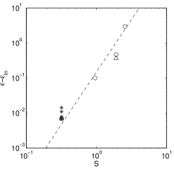
Figure 8: Double logarithmic plot of $\epsilon-\epsilon_{in}$ over $S$ for all three data sets. The symbols are the same as for Fig. 7. The data were fitted (least square) with a function $AS^{2}+BS^{3}$ where $A=10^{-4}$ and $B=0.15$. The dashed line shows $\epsilon-\epsilon_{in}=0.15S^{3}$.

We turn back to the original scope of these investigations to get a better understanding of the return to local isotropy in shear flows. We monitored derivative moments along the parameter curves. The normalized $n$-th order moment of the transverse derivative of the streamwise turbulent velocity component is given by

$$M_{n}(\partial v_{x}/\partial y)=\frac{\langle(\partial v_{x}/\partial y)^{n}\rangle}{\langle(\partial v_{x}/\partial y)^{2}\rangle^{n/2}}\,.$$ (28)

The cases $n=3$ and 4 are studied and the results are summarized in Fig. 9. The flatness ($n=4$) in the lower row grows slowly with Reynolds number and shear parameter, respectively. The Reynolds number trend is thus in agreement with previous investigations pumir1996 ; rogersmoin1986 ; schumachereckhardt2000 ; schumacher2001 . More interesting are the results for the third order moment, the skewness. While it decreases strongly with $Re$ along path I it starts to decline slowly only for the largest values of $Re$ or $S^{*}$ along path II. We note that for both series the Reynolds number is growing while their decay differs. A simple projection onto $Re$ gives thus different results and underlines the idea of taking into account the shear rate as well. This is also supported when plotting all skewness data over $S^{*}$. Now, a trend of the data to have larger skewness values with growing shear parameter is observed (cf. upper right panel of Fig. 9) for the majority of the data set.

Figure 9: Normalized derivative moments $M_{3}(\partial v_{x}/\partial y)$ (upper row) and $M_{4}(\partial v_{x}/\partial y)$ (lower row) as a function of the Reynolds number $Re$ (left column) and the shear parameter $S^{*}$ (right column). The data from series I and II of Table 1 are plotted.

In Ref. 14 the data were discussed with respect to the following question: Is a large Reynolds number really large if the shear parameter is large as well? Large is meant there in the sense of being close to the local isotropy limit. Based on our findings and on (27) one can draw the conclusion that large means then

$$Re\gg(S_{\infty}^{*})^{2}=\frac{1}{C_{2}^{2}C_{3}^{2}C_{4}^{2/3}}\,,$$ (29)

which can be further simplified. For larger $Re$ one would expect $C_{2}\sim{\cal O}(1)$ because this constant is nothing else but the dimensionless energy dissipation rate (see ansatz (21)). A similar argument should hold for $C_{3}$. Thus $Re\gg 1/C_{4}^{2/3}$ would follow eventually. The remaining constant $C_{4}$ which relates the turbulent fluctuations to the shear rate cannot be evaluated by such arguments. The present DNS give $C_{4}\ll 1$ consistently (see the caption of Fig. 7). This can be an interesting point to be answered when the data base is more comprehensive.

V Summary and outlook

We have presented systematic studies of the relation between the shear parameter and the Reynolds number in a turbulent nearly homogeneous shear flow. The present system allows for investigations of a statistically stationary flow with mild fluctuations of the turbulent kinetic energy. The ratio of the turbulence production to the energy dissipation was found to vary around unity and the integral length scale remains well below the box extension. Two parameters, the shear rate $S$ and the energy injection rate $\epsilon_{in}$, were varied by keeping one constant in each case. We monitored the resulting shear parameter $S^{*}$ and Reynolds number $Re$. It was found that they evolve on different pathways across the two-parameter plane. Dimensional estimates are in qualitative agreement with the results of the DNS. They suggest that an asymptotic shear parameter value is reached for the statistically stationary case. The reason for such saturation might be due to the finiteness of the considered volume, namely that the linear mean profile in a homogeneous shear flow causes always an outer flow gradient scale that is beyond the box extensions (strictly speaking this scale is infinite). For any finite system the initially observed self-similar growth of quantities with time is interrupted once $L_{11}$ comes closer to the box size and consequently the shear parameter settles to a finite value.

Another way of such a two-parameter discussion is to use the shear parameter $S^{*}$ and the Corrsin parameter $S_{c}=S\tau_{\eta}$ where the Taylor microscale Reynolds number follows to $R_{\lambda}\simeq S^{*}/S_{c}$. gualtierietal2002 Clearly, our results can be transformed into the latter frame. The large shear limit from Ref. 14, $S^{*}R_{\lambda}^{-1}\gg 1$, would thus translate to $S_{c}\gg 1$ and the local isotropy limit, $S^{*}R_{\lambda}^{-1}\ll 1$, follows to $S_{c}\ll 1$. The latter inequality states then that the shear time scale $S^{-1}$ and the dissipative time scale $\tau_{\eta}$ have to be separated far enough of each other.

It was shown that the third order derivative moments decay with different trends with respect to the Reynolds number when they are monitored along different pathways in the two-parameter plane. There is practically no decay over a wide range when the same data are shown with respect to the the shear parameter. All this might explain the different interpretations of measured moments in terms of a return to local isotropy.

Clearly, the present the Reynolds numbers are mostly small and the data base is rather sparse. It has to become more comprehensive for some reasons: first, one would like to see of these trends persist to higher Reynolds numbers, especially the behavior of the shear parameter $S^{*}$. Secondly, the four parameters $C_{1}$ to $C_{4}$ are assumed to be constant. We do not know if a Reynolds number dependence is hidden there; the current data did not allow for drawing conclusions on that. Thus, we consider this investigation as a starting point. Further extensions beside these two points are possible. The so-called grid forcing scheme gives us a tool into hands which can be extended to cases where spatial and temporal patterns are used for the excitation of turbulent fluctuations, an approach that recently started in terms of active grids in wind tunnels.

- (1) S. B. Pope, Turbulent Flows, (Cambridge University, Cambridge, England, 2000).
- (2) J. L. Lumley, “Similarity and the turbulent energy spectrum,” Phys. Fluids 10, 855 (1967).
- (3) S. Garg and Z. Warhaft, “On small scale statistics in a simple shear flow,” Phys. Fluids 10, 662 (1998).
- (4) M. Ferchichi and S. Tavoularis, “Reynolds number effects on the fine structure of uniformly sheared turbulence,” Phys. Fluids 12, 2942 (2000).
- (5) X. Shen and Z. Warhaft, “The anisotropy of the small scale structure in high Reynolds number () turbulent shear flow,” Phys. Fluids 12, 2976 (2000).
- (6) A. Staicu and W. van de Water, “Small-scale velocity jumps in shear turbulence,” Phys. Rev. Lett. 90, 094501 (2003).
- (7) S. Kurien and K. R. Sreenivasan, “Anisotropic scaling contributions to high-order structure functions in high-Reynolds-number turbulence,” Phys. Rev. E 62, 2206 (2000).
- (8) A. N. Kolmogorov, “The local structure of turbulence in incompressible viscous fluid for very large Reynolds numbers,” Dokl. Akad. Nauk SSSR 30, 9 (1941).
- (9) A. Pumir, “Turbulence in homogeneous shear flows,” Phys. Fluids 8, 3112 (1996).
- (10) J. Schumacher and B. Eckhardt, “On statistically stationary homogeneous shear turbulence,” Europhys. Lett. 52, 627 (2000).
- (11) J. Schumacher, “Derivative moments in stationary homogeneous shear turbulence,” J. Fluid Mech. 441, 109 (2001).
- (12) P. Gualtieri, C. M. Casciola, R. Benzi, G. Amati, and R. Piva, “Scaling laws and intermittency in homogeneous shear flow,” Phys. Fluids 14, 583 (2002).
- (13) T. Ishihara, K. Yoshida, and Y. Kaneda, “Anisotropic velocity correlation spectrum at small scales in a homogeneous turbulent shear flow,” Phys. Rev. Lett. 88, 154501 (2002).
- (14) J. Schumacher, K. R. Sreenivasan, and P. K. Yeung, “Derivative moments in turbulent shear flows,” Phys. Fluids 15, 84 (2003).
- (15) T. Gerz, U. Schumann, and S. E. Elgobashi, “Direct numerical simulations of stratified homogeneous turbulent shear flows,” J. Fluid Mech. 200, 563 (1989).
- (16) R. S. Rogallo, Numerical experiments in homogeneous turbulence, NASA Tech. Mem. 81315 (1981).
- (17) M. M. Rogers and P. Moin, “The structure of the vorticity field in homogeneous turbulent flows,” J. Fluid Mech. 176, 33 (1986).
- (18) V. Yakhot, “A simple model for self-sustained oscillations in homogeneous shear flow,” Phys. Fluids 15, L17 (2003).
- (19) M. J. Lee, J. Kim, and P. Moin, “Structure of turbulence at high shear rate,” J. Fluid Mech. 216, 561 (1990).
- (20) B. Eckhardt and J. Schumacher, “Turbulence and passive scalar transport in a free-slip surface,” Phys. Rev. E 64, 016314 (2001).
- (21) S. Grossmann and D. Lohse, “Scale resolved intermittency in turbulence,” Phys. Fluids 6, 611 (1994).
- (22) R. J. Hill, “Equations relating structure functions of all orders,” J. Fluid Mech. 434, 379 (2001).
- (23) C. M. Casciola, P. Gualtieri, R. Benzi, and R. Piva, “Scale-by-scale budget and similarity laws for shear turbulence,” J. Fluid Mech. 476, 105 (2003).
- (24) V. G. Harris, J. A. H. Graham, and S. Corrsin, “Further experiments in nearly homogeneous turbulent shear flow,” J. Fluid Mech. 81, 657 (1977).
- (25) S. Tavoularis, “Asymptotic laws for transversely homogeneous turbulent shear flows,” Phys. Fluids 28, 999 (1985).
- (26) M. M. Rogers, P. Moin, and W. C. Reynolds, “The structure and modeling of the hydrodynamic and passive scalar fields in homogeneous turbulent shear flow,” Report No. TF-25, Department of Mechanical Engineering, Stanford University (1986).
- (27) F. Waleffe, “On a self-sustaining process in shear flows,” Phys. Fluids 9, 883 (1997).
- (28) J. Schumacher and B. Eckhardt, “Evolution of turbulent spots in a parallel shear flow,” Phys. Rev. E 63, 046307 (2001).
- (29) C. R. Doering, B. Eckhardt, and J. Schumacher, “Energy dissipation in body-forced plane shear flow,” J. Fluid Mech. 494, 275 (2003).
- (30) K. R. Sreenivasan, “An update on the dissipation rate in homogeneous turbulence,” Phys. Fluids 10, 528 (1998).