Time-oscillating Lyapunov modes and auto-correlation functions for quasi-one-
dimensional systems

Abstract

The time-dependent structure of the Lyapunov vectors corresponding to the steps of Lyapunov spectra and their basis set representation are discussed for a quasi-one-dimensional many-hard-disk systems. Time-oscillating behavior is observed in two types of Lyapunov modes, one associated with the time translational invariance and another with the spatial translational invariance, and their phase relation is specified. It is shown that the longest period of the Lyapunov modes is twice as long as the period of the longitudinal momentum auto-correlation function. A simple explanation for this relation is proposed. This result gives the first quantitative connection between the Lyapunov modes and an experimentally accessible quantity.

In recent years, statistical mechanics based on chaotic dynamics has drawn much attention as a scheme to bridge between a deterministic microscopic dynamics and a probabilistic macroscopic theory. In a chaotic system, the difference of two nearby phase space trajectories, the so called Lyapunov vector, diverges rapidly in time, so that a part of the dynamics is unpredictable and a statistical treatment is required. To justify this scheme, much effort has been devoted to discovering the link between macroscopic quantities, such as transport coefficients, and chaotic quantities, such as the Lyapunov vector and the Lyapunov exponent (the exponential rate of divergence or contraction of the magnitude of the Lyapunov vector) Gas98 ; Dor99 . Some works have concentrated upon finding chaotic properties of many-particle systems, and some progress has been made in the search for global properties, like the conjugate pairing rule for the Lyapunov spectrum (the ordered set of Lyapunov exponents) Dre88 .

The stepwise structure of the Lyapunov spectrum is a typical chaotic feature of many-particle systems Del96 . These steps in the spectrum are accompanied by global wavelike structures in the corresponding Lyapunov vectors, or Lyapunov modes Pos00 ; Tan03a ; For04 ; EF04 . The significance of this phenomenon is that this structure appears in the vectors associated with the Lyapunov exponents that are closest to zero, therefore it is connected with the slow macroscopic behavior of the system. Originally, it was observed in systems with hard-core particle interactions, but very recently numerical evidence for Lyapunov modes in a system with soft-core interactions was reported Yan04 . Some analytical approaches, such as random matrix theory Eck00 ; Tan02c , kinetic theory Mcn01b and periodic orbit theory Tan02b , have been used in an attempt to understand this phenomenon.

A clue to understanding the stepwise structure of the Lyapunov spectrum and the Lyapunov modes is in the behavior of the Lyapunov vectors associated with the zero-Lyapunov exponents. In this scenario we claim that the origin of the Lyapunov modes is the translation invariances and conservation laws which dominate the global behavior the system. For a two-dimensional system of $N$ particles in periodic boundary conditions the Lyapunov vectors can be written as $(\delta x,\delta y,\delta p_{x},\delta p_{y})$ where $\delta x$, $\delta y$, $\delta p_{x}$ and $\delta p_{y}$ are the $N$-vectors containing the $x$ and $y$ spatial components, and the $x$ and $y$ momentum components of the Lyapunov vector. For this system there are six degenerate zero-Lyapunov exponents and the Lyapunov modes are linear combinations of one of the basis sets $\{(\Delta,0,0,0)$, $(0,\Delta,0,0)$, $(p_{x},p_{y},0,0)\}$, or $\{(0,0,\Delta,0)$, $(0,0,0,\Delta)$, $(0,0,p_{x},p_{y})\}$, where $0$ is the $N$-dimensional null vector, $\Delta$ is an $N$-dimensional vector with all components equal to $1/\sqrt{N}$, and $p_{x}$ and $p_{y}$ are the $N$-dimensional vectors containing the $x$ and $y$-components of the momentum of each particle Gas98 . Notice that the second basis set is the conjugate of the first, where $(-\delta p,\delta q)$ is the conjugate of $(\delta q,\delta p)$. The first set of basis vectors are associated with spatial and time translational invariance, the second basis set with total momentum and energy conservation. Therefore, in the zero-Lyapunov modes we observe that the sets $\{\delta x_{j}^{(n)}\}$, $\{\delta y_{j}^{(n)}\}$, $\{\delta p_{xj}^{(n)}\}$, $\{\delta p_{yj}^{(n)}\}$, $\{\delta x_{j}^{(n)}/p_{xj},\delta y_{j}^{(n)}/p_{yj}\}$ or $\{\delta p_{xj}^{(n)}/p_{xj},\delta p_{yj}^{(n)}/p_{yj}\}$ can have constant components independent of the particle number index $j$ Tan03a . If the zero-Lyapunov exponents and their Lyapunov vectors can be regarded as the zero-th step then we would expect to see $x$ dependent Lyapunov modes for $k$-vector $k_{n}=2n\pi/L_{x}$ constructed from the basis vectors

$$(0,\sin(k_{n}x_{j}),0,0),(0,\cos(k_{n}x_{j}),0,0),$$ (1)

$$(\sin(k_{n}x_{j}),0,0,0),(\cos(k_{n}x_{j}),0,0,0),$$ (2)

$$(p_{xj}\sin(k_{n}x_{j}),p_{yj}\sin(k_{n}x_{j}),0,0),$$

$$(p_{xj}\cos(k_{n}x_{j}),p_{yj}\cos(k_{n}x_{j}),0,0),$$ (3)

in the quasi-one-dimensional system with periodic boundary conditions Tan03a . However, only the first two of these (1) are observed (as the two-point steps or transverse modes) Tan03a ; EF04 . The second two modes are longitudinal and we notice that the last two basis vectors (3) have time dependent normalisation coefficients. We can remove this time dependence by combining the time-translational invariance mode and the longitudinal modes in a particular way. It is these combined modes that form an approximate basis set for the numerically observed Lyapunov modes

$$\alpha\sin(\omega_{n}t)(p_{xj}\sin(k_{n}x_{j}),p_{yj}\sin(k_{n}x_{j}),0,0)$$

$$+\beta\cos(\omega_{n}t)(\cos(k_{n}x_{j}),0,0,0),$$ (4)

$$\alpha\sin(\omega_{n}t)(p_{xj}\cos(k_{n}x_{j}),p_{yj}\cos(k_{n}x_{j}),0,0)$$

$$+\beta\cos(\omega_{n}t)(\sin(k_{n}x_{j}),0,0,0),$$ (5)

$$\alpha\cos(\omega_{n}t)(p_{xj}\sin(k_{n}x_{j}),p_{yj}\sin(k_{n}x_{j}),0,0)$$

$$+\beta\sin(\omega_{n}t)(\cos(k_{n}x_{j}),0,0,0),$$ (6)

$$\alpha\cos(\omega_{n}t)(p_{xj}\cos(k_{n}x_{j}),p_{yj}\cos(k_{n}x_{j}),0,0)$$

$$+\beta\sin(\omega_{n}t)(\sin(k_{n}x_{j}),0,0,0),$$ (7)

(where $\omega_{n}$ is a frequency) which are normalisable at all times.

Although this scenario for the Lyapunov steps and modes seems to be plausible, convincing evidence is still absent. The wavelike structure in $\delta y_{j}^{(n)}$ as a function of $x_{j}$, the so called the transverse spatial translational invariance Lyapunov mode, is well known Pos00 . This mode is stationary in time, and categorizes one of the two types of Lyapunov steps. Ref. Tan03a showed a mode structure in $\delta y_{j}^{(n)}/p_{yj}$ as a function of $x$, namely the transverse time translational invariance Lyapunov mode. This mode appears as a time-oscillating spatial wavelike structure, and categorizes another type of Lyapunov step. On the other hand, modes of the longitudinal components of the Lyapunov vectors are less convincing. Ref. For04 claims a moving mode structure in $\delta x_{j}^{(n)}$ as a function of $x$, in the same Lyapunov steps as the ones having the mode in $\delta y_{j}^{(n)}/p_{yj}$, but the relation between these two modes are not known. Another important unsolved problem is the time scale of the oscillation of the Lyapunov mode. The period is rather long, often thousands of times as long as the mean free time, and it should correspond to a macroscopic or collective property of the system. However, no direct evidence of this has been reported.

In this letter we show explicit numerical evidence for the time-oscillating wavelike structure of the multiple longitudinal Lyapunov modes, in particular $\delta x_{j}^{(n)}/p_{xj}$ and $\delta x_{j}^{(n)}$ as functions of $x_{j}$ [basis vectors (4), (5), (6), (7)], and clarify the phase relation between them and the mode $\delta y_{j}^{(n)}/p_{yj}$. Further, we present numerical evidence to connect the time-oscillation of the Lyapunov modes to the time-oscillation of the momentum auto-correlation function. Oscillatory behavior has been observed for the momentum auto-correlation function in many macroscopic systems Rah67 ; Han90 , and has its origin in a collective motion of the system Zwa67 . Our central result is that the longest period of oscillation of the Lyapunov modes is twice as long as the period of the longitudinal momentum auto-correlation function. Although the period changes with boundary conditions and with the number of particles $N$, this inter-relation between periods is always satisfied. A possible explanation for this relation is proposed. The auto-correlation function can be observed directly by the neutron and light scattering experiments Han90 ; CL75 and is connected to transport coefficients using linear response theory Kub78 , so this result gives quantitative evidence of a connection between the Lyapunov modes and an experimentally accessible quantity.

One of the difficulties of observing the Lyapunov steps and modes is that numerical calculations of Lyapunov spectra and vectors are very time-consuming, and analytical methods for them are not well established, although there have been some attempts Tan02c ; Tan02b ; New86 . On the other hand, if the above scenario for the Lyapunov steps and modes, based on universal properties like translational invariance and the conservation laws, can be justified, then a simple model should be sufficient to establish its origin. This is the motivation behind the quasi-one-dimensional many-hard-disk system proposed by Tan03a ; Tan03b . It is a very narrow rectangular system where the particle ordering in the longer $x$-direction is invariant. Particle interactions are restricted to nearest neighbors only, so the numerical calculation is much faster than for the full two-dimensional system. Moreover it shows a much longer region of Lyapunov steps and clearer Lyapunov modes, compared with the full two-dimensional system. Another useful technique to get clear Lyapunov steps and modes, is to use hard-wall boundary conditions Tan03a . Although hard-wall boundary conditions break translational invariance and momentum conservation, there is a simple relationship between the Lyapunov steps and modes for systems with different boundary conditions Tan03a . In this letter we use the quasi-one-dimensional many-hard-disk system with hard-wall boundary conditions in the longer $x$ direction and periodic boundary conditions in the shorter $y$ direction [the boundary condition (H,P)]. This system exhibits both types of Lyapunov steps, and is only marginally slower numerically because only the two particles at the ends of the system can collide with the walls. We use units where the mass and disk radius $R$ of each particle is $1$, the total energy is $N$ and the dimensions of the system are chosen as $L_{x}=1.5NL_{y}+2R$ and $L_{y}=2R(1+10^{-6})$, respectively.

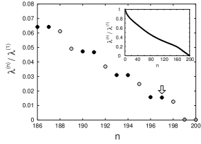
Figure 1: Stepwise structure of the Lyapunov spectrum normalized by the largest Lyapunov exponent $\lambda^{(1)}$ for the quasi-one-dimensional many-hard-disk system with (H,P) boundary condition. The number of particles is $N=100$. The white-filled circles correspond to the stationary modes while the black filled circles are the time-oscillating modes. Inset: The positive branch of the normalized Lyapunov spectrum.

Figure 1 shows the stepwise structure of the normalized Lyapunov spectrum for the quasi-one-dimensional system consisting of $100$ hard-disks with (H,P) boundary condition. In the inset to this figure we show the full normalized spectrum for the positive branch (the negative branch is obtained by the conjugate pairing rule). In this system the spatial translational invariance and the total momentum conservation in the longitudinal direction are violated, and the number of the zero-Lyapunov exponents is $4$. We recognize a clear stepwise structure in which two-point steps and one-point steps appear alternately.

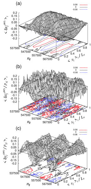
Figure 2: Local time averages of: (a) $\langle\delta x_{j}^{(197)}\rangle_{t}$; (b) $\langle\delta x_{j}^{(197)}/p_{xj}\rangle_{t}$; and (c) $\langle\delta y_{j}^{(197)}/p_{yj}\rangle_{t}$; as functions of the collision number $n_{t}$ and the normalized position $\langle x_{j}\rangle_{t}/L_{x}$ of the $x$-component of the $j$-th particle. The corresponding Lyapunov exponent is indicated by the arrow in Fig. 1. On the bottom of each graph is the projected contour plot of the three dimensional graph at the values $-0.08$ (dotted lines), $0$ (solid lines), and $+0.08$ (broken lines).

One-point steps in the Lyapunov spectrum in Fig. 1 correspond to the stationary mode $\delta y_{j}^{(n)}$ as a function of $x_{j}$ [basis vectors (1)]. This structure is well known as the transverse spatial translational invariant Lyapunov mode, so we omit further discussion here. Figure 2 shows that the Lyapunov modes corresponding to the two-point Lyapunov steps have time-oscillating wavelike mode structures in $\delta x_{j}^{(n)}/p_{xj}$, $\delta y_{j}^{(n)}/p_{yj}$ and $\delta x_{j}^{(n)}$ as functions of $x_{j}$ and the collision number $n_{t}$ with almost the same period $T_{lya}\approx 16300$. More details of this numerical calculation are given elsewhere Tan03a ; Tan04b . By investigating time-dependent Lyapunov modes for the other Lyapunov exponents Tan04b , it is shown that the spatial part of Lyapunov vector components $\delta x$ and $\delta y$ corresponding to the Lyapunov exponents in the $n$-th two-point step are approximately expressed using the basis vectors (5) and (7). Notice however, that for (H,P) boundary conditions $k_{n}=n\pi/L_{x}$. Note that the time-translational invariance Lyapunov modes, that is the terms containing the momentum in basis vectors (4), (5), (6) and (7) have the same structure in the same Lyapunov exponent, and are orthogonal to the longitudinal spatial translational invariant Lyapunov components of the same basis vectors. Large fluctuations in the longitudinal time translational invariance Lyapunov mode, like in Fig. 2(b), come from the terms for the longitudinal spatial translational invariance Lyapunov modes. The spatial nodes of these Lyapunov modes are pinned at the hard-walls Tan03a ; Tan04b .

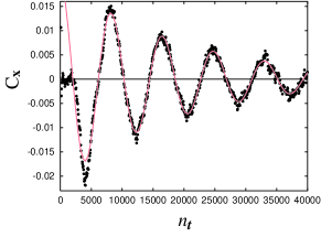
Figure 3: The time-oscillating part of the longitudinal momentum auto-correlation function $C_{x}$, normalized by its initial value, as a function of the collision number $n_{t}$. The system is the same as that used in Figs. 1 and 2. Here, the line is a fit of the data to a sinusoidal function multiplied by an exponential function.

We now discuss the connection between the time-oscillations of Lyapunov modes and the momentum auto-correlation function. Figure 3 shows the longitudinal momentum auto-correlation normalized by its initial value as a function of the collision number $n_{t}$ in the same system as that used in Figs. 1 and 2. Here, an arithmetic average of the auto-correlation functions for $11$ disks in the middle of the system (far from the hard walls) is taken. This auto-correlation function initially shows a simple exponential damping, as discussed elsewhere Tan04b , so that part is omitted in Fig. 3. A clear time-oscillating behavior is observed in Fig. 3 that is nicely fitted to a sinusoidal function times an exponential decay. This fitting gives the oscillating period $T_{acf}\approx 8290$, which suggests the approximate relation

$$T_{lya}\approx 2T_{acf}$$ (8)

between the oscillating periods of the Lyapunov mode and the momentum auto-correlation function. Numerically this relation is satisfied irrespective of the number of particles and boundary conditions Tan04b .

The relation (8) can be obtained from the following physical argument. Consider the Fourier space auto-correlation function $<\tilde{p}_{x}(t)^{*}\;\tilde{p}_{x}(0)>$ for the longitudinal component $\tilde{p}_{x}(t)$ of the momentum that oscillates with frequency $\omega_{acf}$, namely $<\tilde{p}_{x}(t)^{*}\;\tilde{p}_{x}(0)>\sim\phi(t)\;\exp\{i\omega_{acf}t\},$ where $\phi(t)$ is the damping factor and the suffix ^∗ indicates the complex conjugate. On the other hand we have a term for the longitudinal time translational invariance Lyapunov mode, like the first component of the basis vectors (5) and (7), as $\delta\tilde{q}_{x}\sim\psi_{1}(t)\tilde{p}_{x}(t)\exp\{i\omega_{lya}t\}$ with a frequency $\omega_{lya}$, where $\psi_{1}(t)$ is an amplitude factor. We assume that if the quantity $\delta\tilde{q}_{x}$ oscillates persistently in time, then its auto-correlation function $<\delta\tilde{q}_{x}(t)^{*}\;\delta\tilde{q}_{x}(0)>$ should also oscillate in time with the same frequency $\omega_{lya}$, namely $<\delta\tilde{q}_{x}(t)^{*}\;\delta\tilde{q}_{x}(0)>\sim\psi_{2}(t)\exp\{i\omega_{lya}t\}$ with a damping factor $\psi_{2}(t)$. (Actually we can show that the auto-correlation function for the spatial longitudinal component of the Lyapunov vector oscillates with the same frequency as the Lyapunov vector component itself in the quasi-one-dimensional system Tan04b .) It follows from these equations and the assumption that $\psi_{2}(t)\exp\{i\omega_{lya}t\}\sim\psi_{1}(t)^{*}\;\psi_{1}(0)\;\phi(t)\;\exp\{i(\omega_{acf}-\omega_{lya})t\}$, that $\omega_{lya}\sim\omega_{acf}/2$. The frequency is inversely proportional to the oscillation period, so we obtain relation (8).

In conclusion, we have discussed time-oscillating Lyapunov modes and the momentum auto-correlation function in quasi-one-dimensional many-hard-disk systems. We clarified the phase relation between components of multiple time-dependent Lyapunov modes, one coming from the longitudinal spatial translational invariance and another from the time translational invariance. We showed that the longest time-oscillating period of the Lyapunov modes is almost twice as long as the time-oscillating period of the longitudinal momentum auto-correlation function. The momentum auto-correlation can be measured through experiments like the neutron and light scattering experiments, so our result give a direct connection between the Lyapunov mode with an experimentally accessible quantity.

We are grateful for the financial support for this work from the Australian Research Council. One of the authors (T. T.) also appreciates the financial support by the Japan Society for the Promotion Science.

References

- (1) P. Gaspard, Chaos, scattering and statistical mechanics (Cambridge University press, 1998).
- (2) J. R. Dorfman, An introduction to chaos in nonequilibrium statistical mechanics (Cambridge University press, 1999).
- (3) U. Dressler, Phys. Rev. A 38, 2103 (1988); D. J. Evans, E. G. D. Cohen, and G. P. Morriss, Phys. Rev. A 42, 5990 (1990); C. P. Dettmann and G. P. Morriss, Phys. Rev. E 53, R5545 (1996); T. Taniguchi and G. P. Morriss, Phys. Rev. E 66, 066203 (2002).
- (4) Ch. Dellago, H. A. Posch, and W. G. Hoover, Phys. Rev. E 53, 1485 (1996).
- (5) H. A. Posch and R. Hirschl, in Hard ball systems and the Lorentz gas, edited by D. Szász (Springer, Berlin, 2000), p. 279.
- (6) T. Taniguchi and G. P. Morriss, Phys. Rev. E 68, 026218 (2003).
- (7) C. Forster, R. Hirschl, H. A. Posch, and W. G. Hoover, Physica D 187, 294 (2004).
- (8) J. -P. Eckmann, C. Forster, H. A. Posch and E. Zabey, e-print nlin.CD/0404007.
- (9) H. Yang and G. Radons, e-print nlin.CD/0404027.
- (10) J. -P. Eckmann and O. Gat, J. Stat. Phys. 98, 775 (2000).
- (11) T. Taniguchi and G. P. Morriss, Phys. Rev. E 65, 056202 (2002).
- (12) S. McNamara and M. Mareschal, Phys. Rev. E 64, 051103 (2001); A. S. de Wijn and H. van Beijeren, e-print nlin.CD/0312051.
- (13) T. Taniguchi, C. P. Dettmann, and G. P. Morriss, J. Stat. Phys. 109, 747 (2002).
- (14) A. Rahman, Phys. Rev. Lett. 19, 420 (1967); W. E. Alley, B. J. Alder, and S. Yip, Phys. Rev. A 27, 3174 (1983).
- (15) J. P. Hansen and I. R. McDonald, Theory of simple liquids, 2nd ed. (Academic press, 1990).
- (16) R. Zwanzig, Phys. Rev. 156, 190 (1967).
- (17) J. R. D. Copley and S. W. Lovesey, Rep. Prog. Phys. 38, 461 (1975); W. Schaertl and C. Roos, Phys. Rev. E 60, 2020 (1999).
- (18) R. Kubo, M. Toda, and N. Hashitsume, Statistical physics II, nonequilibrium statistical mechanics (Springer-Verlag, Berlin Heidelberg, 1985).
- (19) C. M. Newman, Commun. Math. Phys. 103, 121 (1986).
- (20) T. Taniguchi and G. P. Morriss, Phys. Rev. E 68, 046203 (2003).
- (21) T. Taniguchi and G. P. Morriss, unpublished.