Nonlinear stability of oscillatory wave fronts in chains of coupled oscillators

Abstract

We present a stability theory for kink propagation in chains of coupled oscillators and a new algorithm for the numerical study of kink dynamics. The numerical solutions are computed using an equivalent integral equation instead of a system of differential equations. This avoids uncertainty about the impact of artificial boundary conditions and discretization in time. Stability results also follow from the integral version. Stable kinks have a monotone leading edge and move with a velocity larger than a critical value which depends on the damping strength.

I Introduction

The dynamics of waves in chains of coupled oscillators is the key to understanding the motion of defects in many physical and biological problems: motion of dislocations fk ; nab67 or cracks sle81 in crystalline materials, atoms adsorbed on a periodic substrate cha95 , motion of electric field domains and domain walls in semiconductor superlattices bon02 , pulse propagation through myelinated nerves sleeman or cardiac cells kee98 … A peculiar feature of these spatially discrete systems is that wave fronts and pulses get pinned for entire intervals of a control parameter such as an external force. Typically, wave fronts do not move unless the external force surpasses a control value. Such is the case with the static and dynamic Peierls stresses in dislocation dynamics hob65 ; nab67 or the dynamic and static friction coefficients ger01 in continuum mechanics. Pinning and motion of wave fronts also explain the relocation of static electric field domains and the self-oscillations of the current in semiconductor superlattices bon02 .

Wave front motion in systems of nonlinear oscillators modeling these phenomena are easier to analyze in the overdamped case, and less so if inertia is important. In the presence of inertia, the wrong choice of boundary conditions or the numerical method may suppress important solutions of the original system or yield spurious oscillations. Thus two problems that are important in all spatially discrete systems acquire even more importance: how do we find wave fronts? and, what are their stability properties?

We have solved the first problem in a recent work wavy by choosing a damped system of oscillators with a piecewise linear source term, see also atk65 ; sle81 ; truski . Our results show explicitly the existence of kinks with oscillatory profiles for systems with little or no damping. In the latter case, these wave fronts have at least one tail with non decaying oscillations that extend to infinity. Depending on the control parameter, branches of oscillatory wave fronts may exist, coexisting for entire intervals of the external force and even coexisting with pinned wave front solutions. These facts, long-lived oscillatory profiles and coexistence of wave front branches, highlight the importance of ascertaining the stability properties of these solutions. This is not easy and not many results are known.

To be precise, let us consider oscillator chain:

$$mu_{n}^{\prime\prime}\!+\!\alpha u_{n}^{\prime}\!=\!K(u_{n+1}-2u_{n}+u_{n-1})\!-\!V^{\prime}(u_{n})\!+\!W.$$ (1)

We nondimensionalize the model by choosing the time scale $\sqrt{{ma^{2}\over v_{m}}}$, where $a$ is the interatomic distance, $m$ is the mass and $v_{m}$ the strength of the on-site potential. For a piecewise parabolic potential, the nondimensional equation is:

$$u_{n}^{\prime\prime}+\gamma u_{n}^{\prime}=D(u_{n+1}-2u_{n}+u_{n-1})-g(u_{n})+F,$$ (2)

$$g(s)=\left\{\begin{array}[]{ll}s\quad s<{1\over 2}\\ s-1\quad s\geq{1\over 2}.\end{array}\right.$$ (5)

Here $\gamma$ and $D$ are the ratios between friction and inertial forces, and between the strengths of the harmonic and on-site potentials, respectively. $F=Wa/v_{m}$. Atkinson and Cabrera atk65 conjectured that only two branches of kinks are stable for (2)-(5):

• a branch of static kinks for values of the control parameter $|F|$ below an static threshold $F_{cs}(D),$

• a branch of traveling kinks for $|F|$ above a dynamic threshold $F_{cd}(\gamma,D)\leq F_{cs}(D)$, with speeds $c$ larger than a minimum speed $c_{cd}(\gamma,D)$. This family has a distinctive feature compared to eventual slower waves wavy : the leading edge of the kink is monotone whereas the trailing edge may develop oscillations.

The values $F_{cs}$ and $F_{cd}$ correspond to the static and dynamic Peierls stresses of the literature on dislocations nab67 . In the overdamped limit $\gamma\rightarrow\infty$, $F_{cs}=F_{cd}$ and stable wave fronts can be found with arbitrarily small speeds fat98 .

In a previous paper wavy , we checked numerically the validity of Atkinson and Cabrera’s conjecture. This is a delicate affair and further analytical work is clearly desirable. In fact, most numerical studies of kink propagation truncate the infinite chain to a finite chain, fix some boundary conditions and then use a Runge-Kutta solver (or variants) to investigate the dynamics of kink-like initial configurations. For instance, Peyrard and Kruskal pey84 applied this procedure to study kinks in the conservative Frenkel-Kontorova model, including friction near the ends of the truncated chain in an attempt to avoid reflections. On the other hand, our analytical work wavy shows that traveling kinks oscillate with almost uniform amplitude even for small damping. Then, artificial boundary conditions and time discretization may greatly distort their shape and dynamics. In fact, using Runge-Kutta methods to solve equation (2) with constant boundary conditions generates reflections at the boundary, as shown in Figure 1, after a waiting time depending on the size of the lattice. Such oscillations end up distorting the right tail and may completely alter the shape of the kink giving rise to a complex oscillatory pattern.

A good way to avoid the spurious effects of inappropiate boundary conditions is to recast (2) as an integral equation. Integral reformulations provide an analytical expression for the solutions of (2) which we use to develop new numerical algorithms. Spurious pinning and spurious oscillations are suppressed. The introduction of these numerical methods based on integral reformulations of (2) is one of our main results.

The main analytical results of this paper concern the nonlinear stability of stationary and traveling wave fronts in chains of oscillators. Besides leading to good numerical methods, we have also used the integral equation formulation to investigate the nonlinear stability of wave front patterns. We provide a criterion to decide whether certain kink-like initial configurations evolve into stable wave front patterns. In discrete overdamped models the nonlinear stability of traveling wave fronts follows from comparison principles. This strategy was applied to the study of domain walls in discrete drift-diffusion models for semiconductor superlattices in car00 .

Common belief is that comparison principles do not hold in models with inertia. This belief is wrong. How can we asses the stability of traveling wave fronts in such models? For large damping, we can directly compare solutions of (2) using its equivalent formulation as an integral equation thanks to the positivity of the Green functions. As the damping decreases, we can ignore the oscillatory tails of the fronts and compare the monotone leading edges of the solutions, which drive their motion. The process of comparing solutions is technically more complex than in the overdamped case because the Green functions change sign, and the fronts have oscillatory wakes. Summarizing, there are two key ingredients for stability. First, the leading edges of the fronts have to be monotone. Second, the Green functions of the linear problem must be positive for an initial time interval, of duration comparable to the time the front needs to advance one position. This restricts the possible values of the propagation speed for small damping: only fast kinks are shown to be stable. Our methods are quite general and can be extended to Frenkel-Kontorova models with smooth sources preprint at the cost of technical complications.

The paper is organized as follows. In section 2 we introduce a numerical algorithm and discuss the stability of static kinks. The stability theory for traveling kinks is presented in Section 3. In section 4 we discuss the role of oscillating Green functions in the appearance of static and dynamic thresholds due to coexistence of stable static and traveling waves. In section 5 we briefly comment on extensions to oscillator chains with smooth cubic sources. Section 6 contains our conclusions. Basic details on the pertinent Green functions are recalled in Appendices A and B. Proofs of our main stability results can be found in Appendices C and D.

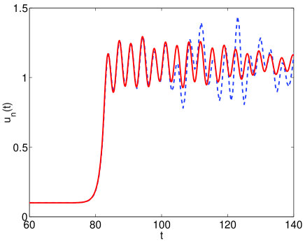
Figure 1: Trajectory $u_{n}(t)$ computed by solving a truncated system of differential equations (dashed) and by integral expressions (solid) for $\gamma=0.02$, $D=4$, $F=0.1$, $n=-70$.

II Static kinks

The stationary wave fronts $s_{n}$ for (2) increase from $s_{-\infty}=F$ to $s_{\infty}=1+F$ and solve the second order difference equation:

$$D(s_{n+1}-2s_{n}+s_{n-1})-s_{n}+H\big{(}s_{n}-{1\over 2}\big{)}+F=0$$ (6)

in which $H(x)$ is the Heaviside unit step function. These fronts are translation invariant. We fix their position by setting $s_{0}<{1\over 2}<s_{1}$. Then, $s_{n}=F+ar^{n}$ for $n\leq 0$ and $s_{n}=1+F-br^{-n}$ for $n\geq 1$, where $r={2D+1+\sqrt{4D+1}\over 2D}$. Inserting these formulas in equation (6) for $n=0$ and $n=1$, we find $a$ and $b$. Our construction of the stationary fronts $s_{n}$ is consistent with the restriction $s_{0}<{1\over 2}<s_{1}$ when $|F|\leq F_{cs}(D)$. Figure 2 (a) shows a static wave front for $D=4$ and $F=0.05$. As $D$ grows, the number of points in the transition layer between the constants increases.

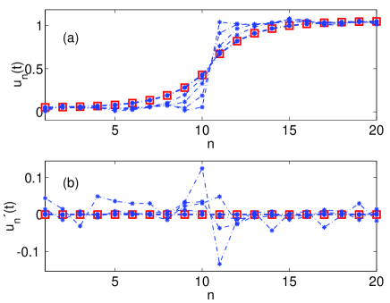
Figure 2: Convergence to a static kink $s_{n}$ when $D=4$, $\gamma=10$ and $F=0.05$: (a) asterisks $u_{n}(t)$, squares $s_{n}$, (b) asterisks $u_{n}^{\prime}(t)$, squares $s_{n}^{\prime}=0$.

II.1 Stability

A stationary wave front $s_{n}$ is stable for the dynamics (2) when chains initially close to $s_{n}$ remain near $s_{n}$ for all $t>0$, as shown in Figure 2. The initial states chosen in this figure are $u_{n}^{0}=F+\delta^{0}_{n}$ when $n\leq 0$, $u_{n}^{0}=1+F+\delta_{n}$ when $n\geq 1$ and $u_{n}^{1}=\delta_{n}^{1}$. Both $\delta_{n}^{1}$ and $\delta_{n}^{0}$ are small random perturbations.

To find the stable profiles, we proceed as follows. Let $u_{n}^{0}$ and $u_{n}^{1}$ be the initial position and velocity of the chain. In terms of Green functions calculated in Appendix A, $u_{n}(t)$ is given by (82) with $f_{k}(t)=F+H\big{(}u_{k}(t)-{1\over 2}\big{)}:$

$$\begin{array}[]{r}u_{n}(t)=\sum_{k}G_{nk}^{0}(t)u_{k}^{1}+\sum_{k}G_{nk}^{1}(t)u_{k}^{0}\\ +\int_{0}^{t}\sum_{k}G_{nk}^{0}(t-z)H\big{(}u_{k}(z)-{1\over 2}\big{)}dz\\ +F\int_{0}^{t}\sum_{k}G_{nk}^{0}(t-z)dz.\end{array}$$ (10)

If initially $u_{k}^{0}<{1\over 2}$ for $k\leq 0$, $u_{k}^{0}>{1\over 2}$ for $k\geq 1$:

$$\begin{array}[]{r}u_{n}(t)=\sum_{k}\Big{[}G_{nk}^{0}(t)u_{k}^{1}+G_{nk}^{1}(t)u_{k}^{0}\Big{]}+\\ \int_{0}^{t}\sum_{k>0}G_{nk}^{0}(t-z)dz+F\int_{0}^{t}\sum_{k}G_{nk}^{0}(t-z)dz\end{array}$$ (13)

as long as $u_{k}(t)<{1\over 2}$ when $k\leq 0$, $u_{k}(t)>{1\over 2}$ when $k\geq 1$. For $|F|<F_{cs}(D)$, the static wave front $s_{n}$ with $s_{0}<{1\over 2}<s_{1}$ is a solution of equation (10) that satisfies:

$$\begin{array}[]{r}s_{n}=\sum_{k}G_{nk}^{1}(t)s_{k}+\int_{0}^{t}\sum_{k>0}G_{nk}^{0}(t-z)dz\\ +F\int_{0}^{t}\sum_{k}G_{nk}^{0}(t-z)dz\end{array}$$ (16)

for all $t>0$. Subtracting (16) from (13), we obtain:

$$u_{n}(t)-s_{n}=\sum_{k}\Big{[}G_{nk}^{0}(t)u_{k}^{1}+G_{nk}^{1}(t)(u_{k}^{0}-s_{k})\Big{]}$$ (17)

This expression holds for $t>0$ provided $u_{n}(t)-{1\over 2}$ does not change sign for any $n$ and $t>0$. For which profiles $u_{n}(t)$ is this true? Let us select the initial state of the chain in the set:

$$\begin{array}[]{r}\sum_{-\infty}^{\infty}|u_{n}^{0}-s_{n}|<M,\quad\sum_{-\infty}^{\infty}|u_{n}^{1}|<M\\ M<R\;{\rm Min}(1,{1\over C_{0}+C_{1}})\end{array}$$ (20)

with $R={\rm Min}(|s_{0}-{1\over 2}|,s_{1}-{1\over 2})$ and $C_{0},C_{1}$ to be defined below. For $\gamma>0$, we show in Appendix B that $|G_{nk}^{0}|\leq C_{0}e^{-\eta t}$, $|G_{nk}^{1}|\leq C_{1}e^{-\eta t}$ with $\gamma>0$. This boundedness property of the Green functions and (20) yield:

$$|u_{n}(t)-s_{n}|\leq(C_{0}+C_{1})e^{-\eta t}M$$ (21)

Then, $|u_{n}(t)-s_{n}|<R$ and $u_{n}(t)-{1\over 2}$ cannot change sign for any $t>0$. Moreover, $u_{n}(t)\rightarrow s_{n}$ as $t\rightarrow 0$.

In summary, the static kinks are exponentially and asymptotically stable in the damped case. Their basin of attraction includes all initial configurations $u_{n}^{0}$ and $u_{n}^{1}$ selected according to (20). In the conservative case, the static kinks are merely stable, but not asymptotically stable, because the previous argument with $\gamma=0$, $\eta=0$, $C_{0}=C_{1}=1$ only yields $|u_{n}(t)-s_{n}|\leq 2M$ for all times.

In the continuum limit $D\rightarrow\infty$, the number of points in the transition layer between constants increases and the distance between points decreases. Then, $s_{0}$ and $s_{1}$ tend to ${1\over 2}$ and the set of states (20) attracted by $s_{n}$ shrinks as $D$ grows. It becomes more likely that initial kinks in the chain propagate for a while and finally become pinned at some shifted static kink $v_{n}=s_{n+l}$, $v_{-l}<{1\over 2}<v_{-l+1}$.

II.2 Numerical algorithm

Formula (10) can be used to compute numerically the dynamics of the chain. However, the computational cost is high, due to the integral terms and the Green functions. In this section, we exploit the static front solutions $s_{n}$ to reduce the cost and derive new formulae for $u_{n}(t)$ which clarify the dynamics of the chain.

We will focus on initial kink-like initial states that generate ordered dynamics: $u_{k}(t)-{1\over 2}$ changes sign in an ordered way as the kink advances. Once the kink has passed, the configuration of the chain is close to a shifted static kink. That is why we use static kinks to obtain simplified expressions for $u_{n}(t)$. For instance, let us choose a piecewise constant initial profile $u_{n}^{0}=F$ for $n\leq 0$ and $u_{n}^{1}=1+F$ for $n\geq 1,$ with $u_{n}^{1}=0$. For $F>0$, Figure 3 shows that $u_{-k}(t)-{1\over 2}$ change sign at time $t_{k}$, $k=0,1,....$, with $t_{0}<t_{1}<...<t_{k}<...$. Eventually, the kink may get pinned at some static configuration and this process stops at some $k$. We then use a slightly modified version of the integral expression (16) for the static wave fronts to successively remove the integral terms in (10) and obtain simple formulae for $u_{n}(t)$ similar to (17). In this way, we find a relatively cheap algorithm for the computation of $u_{n}(t)$.

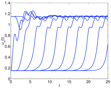
Figure 3: Trajectories $u_{n}(t)$, $n=8,4,0,-4,...$ when $D=4$, $\gamma=0.4$, $F=0.15$.

Let us describe the algorithm for $F\geq 0$ and an initial step-like state $u_{n}^{0}$ with $u_{0}^{0}<{1\over 2}<u_{1}^{0}$, as in Figure 3. We must distinguish two cases: $0<F\leq F_{cs}(D)$ and $F>F_{cs}(D).$

II.2.1 Case $0<F\leq F_{cs}(D)$

In this case, the stationary wave fronts can be used to generate a faster algorithm for obtaining $u_{n}(t)$. we remove the integrals in (10) by using the static wave front solution of (2), $s_{n}$, such that $s_{0}<{1\over 2}<s_{1}$.

Initial stage. Formula (17) allows to compute $u_{n}(t)$ up to the time $t_{0}$ at which $u_{0}(t)-{1\over 2}$ changes sign. For $t>t_{0}$ we compute $u_{n}(t)$ using as initial data $u_{n}(t_{0})$ and $u_{n}^{\prime}(t_{0})$ at $t_{0}$. The later is obtained differentiating (17):

$$\begin{array}[]{l}u_{n}^{\prime}(t_{0})=\sum_{k}\Big{[}{dG_{nk}^{0}(t_{0})\over dt}u_{k}^{1}+{dG_{nk}^{1}(t_{0})\over dt}(u_{k}^{0}-s_{k})\Big{]}.\end{array}$$ (23)

For $t_{0}<t\leq t_{1}$, equation (10) becomes:

$$\begin{array}[]{l}u_{n}(t)\!=\!\sum_{k}\!\Big{[}G_{nk}^{0}(t-\!t_{0})u_{k}^{\prime}(t_{0})\!+\!G_{nk}^{1}(t-\!t_{0})u_{k}(t_{0})\Big{]}\\ +\int_{t_{0}}^{t}\sum_{k>-1}G_{nk}^{0}(t-z)dz\!+\!F\int_{t_{0}}^{t}\sum_{k}G_{nk}^{0}(t-z)dz\end{array}$$ (26)

Now, $u_{-1}(t_{0})<{1\over 2}<u_{0}(t_{0})$ and we must use the shifted stationary solution $v_{n}=s_{n+1}$, that satisfies $v_{-1}<{1\over 2}<v_{0}$. Observing that $s_{n+1}$ solves (2) with initial data $s_{n+1},0$ at time $t_{0}$ we obtain the formula:

$$\begin{array}[]{l}s_{n+1}\!=\!\sum_{k}G_{nk}^{1}(t-t_{0})s_{k+1}+F\int_{t_{0}}^{t}\sum_{k}G_{nk}^{0}(t-z)dz\\ +\int_{t_{0}}^{t}\sum_{k>-1}G_{nk}^{0}(t-z)dz\end{array}$$ (29)

Subtracting (29) from (26) we find:

$$\begin{array}[]{l}u_{n}(t)=s_{n+1}+\sum_{k}G_{nk}^{0}(t-t_{0})u_{k}^{\prime}(t_{0})\\ +\sum_{k}G_{nk}^{1}(t-t_{0})(u_{k}(t_{0})-s_{k+1}),\end{array}$$ (32)

up to the time $t_{1}$ at which $u_{-1}(t)-{1\over 2}$ changes sign.

Generic step. Once we have computed the time $t_{l}$ at which $u_{l}(t)-{1\over 2}$ changes sign, we calculate the new initial data $u_{n}(t_{l})$ and $u_{n}^{\prime}(t_{l})$:

$$\begin{array}[]{r}u_{n}(t_{l})=s_{n+l}+\sum_{k}G_{nk}^{0}(t_{l}-t_{l-1})u_{k}^{\prime}(t_{l})\\ +\sum_{k}G_{nk}^{1}(t_{l}-t_{l-1})(u_{k}(t_{l})-s_{k+l}),\end{array}$$ (35)

$$\begin{array}[]{r}u_{n}^{\prime}(t_{l})=\sum_{k}{dG_{nk}^{0}\over dt}(t_{l}-t_{l-1})u_{k}^{\prime}(t_{l})+\\ \sum_{k}{dG_{nk}^{1}\over dt}(t_{l}-t_{l-1})(u_{k}(t_{l})-s_{k+l}).\end{array}$$ (38)

Then the evolution of the chain for $t>t_{l}$ is given by the formula:

$$\begin{array}[]{r}u_{n}(t)=s_{n+l+1}+\sum_{k}G_{nk}^{0}(t-t_{l})u_{k}^{\prime}(t_{l})+\\ \sum_{k}G_{nk}^{1}(t-t_{l})(u_{k}(t_{l})-s_{k+l+1}),\end{array}$$ (41)

until either $u_{-(l+1)}(t)-{1\over 2}$ or $u_{-l}(t)-{1\over 2}$ change sign. If $u_{-(l+1)}(t)-{1\over 2}$ changes its sign at a time $t_{l+1}$, we start a new step using $s_{n+l+1}$ to compute $u_{n}(t)$. If $u_{-l}(t)-{1\over 2}$ reverses its sign at a time $t_{l+1}$, we start a new step using $s_{n+l-1}$ to compute $u_{n}(t)$.

II.2.2 Case $F>F_{cs}(D)$

In this case, it is convenient to remove the integral in Eq. (10) by using as $s_{n}$ the static wave front solution of (2) corresponding to an applied force $F=F_{cs}(D)$, and such that $s_{0}<{1\over 2}<s_{1}$. Recall that there are no stationary wave fronts for $F>F_{cs}$.

Initial stage. Subtracting (16) at $F_{cs}(D)$ from (13) we find:

$$\begin{array}[]{l}u_{n}(t)=s_{n}+\sum_{k}G_{nk}^{0}(t)u_{k}^{1}+\sum_{k}G_{nk}^{1}(t)(u_{k}^{0}-s_{k})\\ +(F-F_{cs})\int_{0}^{t}\sum_{k}G_{nk}^{0}(t-z)dz\end{array}$$ (44)

The remaining integral term can be removed by observing that $1$ is a solution of (2) with $F=0$ and initial data $u_{n}(0)=1,$ $u_{n}^{\prime}(0)=0$:

$$1=\sum_{k}G_{nk}^{1}(t)+\int_{0}^{t}\sum_{k}G_{nk}^{0}(t-z)dz$$ (45)

Multiplying (45) by $(F-F_{cs})$ and inserting the result in (44) we obtain:

$$\begin{array}[]{r}u_{n}(t)=s_{n}+(F-F_{cs})+\sum_{k}G_{nk}^{0}(t)u_{k}^{1}\\ +\sum_{k}G_{nk}^{1}(t)(u_{k}^{0}-s_{k}-(F-F_{cs}))\end{array}$$ (48)

up to the time $t_{0}$ at which $u_{0}(t)-{1\over 2}$ changes sign. For $t>t_{0}$:

$$\begin{array}[]{l}u_{n}(t)=s_{n+1}+(F-F_{cs})+\sum_{k}G_{nk}^{0}(t-t_{0})u_{k}^{\prime}(t_{0})\\ +\sum_{k}G_{nk}^{1}(t-t_{0})(u_{k}(t_{0})-s_{k+1}-(F-F_{cs})),\\ u_{n}^{\prime}(t_{0})\!=\!\!\sum_{k}\!\!\Big{[}{dG_{nk}^{0}(t_{0})\over dt}u_{k}^{1}\!+\!{dG_{nk}^{1}(t_{0})\over dt}(u_{k}^{0}\!-\!s_{k}\!-\!F\!+\!F_{cs}\!)\!\Big{]},\end{array}$$ (52)

up to the time $t_{1}$ at which $u_{-1}(t)-{1\over 2}$ changes sign.

Generic step. Similar to the generic step for $F\leq F_{cs}$ but replacing $s_{n}$ by $s_{n}+(F-F_{cs})$.

II.2.3 Numerical implementation

We will use (41)-(38) and (52) to study the dynamics of the chain in Section III. Due to translational invariance $G_{nk}^{0}=G_{n-k,0}^{1}$ and $G_{nk}^{1}=G_{n-k,0}^{1}$. To calculate $u_{n}(t)$, we only need to compute $G_{n0}^{0}(t)$, $G_{n0}^{1}(t)$ for a time interval $[0,T]$, $T\leq{\rm max}_{l}|t_{l+1}-t_{l}|$ and for $|n|\leq N$, where $N$ is sufficiently large. We calculate the integrals $G_{n0}^{0}(t)$, $G_{n0}^{1}(t)$, ${dG_{n0}^{0}(t)\over dt}$ and ${dG_{n0}^{1}(t)\over dt}$ by means of the Simpson rule, choosing a step smaller than the period of the oscillatory factors. The value $N$ is selected so as to make the error introduced by the truncated series $\sum_{|n-k|\leq N}$ sufficiently small. This is possible because the Green functions and their derivatives decay as $|n-k|$ grows.

A more general version of our algorithm will be presented elsewhere preprint .

III Stability of traveling kinks

In this section we introduce a strategy to study the stability of traveling wave fronts in (2).

Traveling wave fronts are constructed by inserting $w_{n}(t)=w(n-ct)$ in (2) to produce a nonlinear eigenvalue problem for the profile $w(x)$ and the speed $c$. Assuming $w(x)<{1\over 2}$ for $x<0$ and $w(x)>{1\over 2}$ for $x>0$, the problem becomes linear. The wave profiles are computed as contour integrals, imposing $w(0)={1\over 2}$ to find a relationship between $c$ and $F$ atk65 ; wavy . The law $F(c)$ and the shape of the wave profiles are controlled by the poles contributing to the contour integrals. The relevant poles depend on the strength of the damping. For large damping, we have complex poles with large imaginary parts. The dependence law $F(c)$ is monotonically increasing and the wave profiles are monotone. For small damping, poles with small imaginary parts become relevant, in increasing number as the speed $c$ decreases. The function $F(c)$ oscillates for small speeds. Different oscillatory wave profiles with different speeds may coexist for the same $F$. At zero damping, those poles become real and the wave profiles develop non decaying oscillations. For some ranges of speeds, the waves constructed in this way violate the restriction $w(x)<{1\over 2}$ for $x<0$ and $w(x)>{1\over 2}$ for $x>0$. Those ranges should be investigated with a modified technique allowing for a finite number of turning points.

Complex variable methods yield families of explicit wave solutions but give no information on their stability. Numerical tests wavy and physical context atk65 suggest the stability of traveling kinks that have monotone leading edges and large enough speeds. Figures (4)-(6) depict the wave profiles for decreasing $\gamma$. We now confirm that these wave fronts are stable. The travelling wave $w_{n}(t)$ is stable for the dynamics of the chain when the solutions $u_{n}(t)$ of (2) remain near $w_{n}(t)$ for all $t>0$ if the initial states $u_{n}^{0}$, $u_{n}^{1}$ are chosen near $w_{n}(0),w_{n}^{\prime}(0)$. Controlling the evolution of $u_{n}(t)$ is more or less difficult depending on the properties of the Green functions. We distinguish two cases: positive Green functions (large damping) and oscillatory Green functions (small damping).

III.1 Strong damping

For large damping $\gamma^{2}\gg 4$, we know that the wave front profiles are monotonically increasing and that the Green functions are positive and decay exponentially in time (cf. Appendix B). The main result of this section is the following stability theorem, whose proof can be found in Appendix C:

Theorem. Let us select the wave front profile so that $w_{n}(t)=w(n-ct-{1\over 2})$, with $c<0$, and $F>0$. If we choose the initial states for (2), $u_{n}^{1}$ and $u_{n}^{0}$, in the set:

$$w_{n}(-\tau)<u_{n}^{0}<w_{n}(\tau),\quad 0<\tau\ll{1\over 2|c|}$$ (53)

$$\begin{array}[]{l}|w_{n}^{\prime}(-\tau)-u_{n}^{1}|\ll u_{n}^{0}-w_{n}(-\tau)\\ |w_{n}^{\prime}(\tau)-u_{n}^{1}|\ll w_{n}(\tau)-u_{n}^{0}\end{array}$$ (56)

then

$$w_{n}(t-\tau)<u_{n}(t)<w_{n}(t+\tau)$$ (57)

for all $n$ and $t>0$.

In other words, if the initial oscillator configuration is sandwiched between two wave front profiles with different phase shifts, $w_{n}(-\tau)$ and $w_{n}(\tau)$, (with a sufficiently small $\tau$), then the oscillator chain remains trapped between the two shifted profiles $w_{n}(t-\tau)$ and $w_{n}(t-\tau)$ forever, provided $|u_{n}^{1}-w_{n}^{\prime}(0)|$ is sufficiently small. This implies the dynamical stability of the wave. The more involved argument explained in Section III.2 for conservative dynamics can be used to prove that the wave fronts are also asymptotically stable.

Furthermore, the basin of attraction of a particular traveling wave is larger than (53) - (56), as shown in Figures 4-5 for $F>F_{cs}(D)$. The initial oscillator configuration in this figure is a step function, $u_{n}^{0}=F$ for $n\leq 0$ and $u_{n}^{0}=1+F$ for $n\geq 1$, with a superimposed small random disturbance. The initial velocity profile fluctuates randomly about zero with a small amplitude. After an initial transient, the trajectories get trapped between advanced wave fronts, $w_{n}(t+\tau)$, and delayed wave fronts, $w_{n}(t-\tau)$. Moreover, they converge to a shifted wave front, $w_{n}(t+\alpha)$, as $t\rightarrow\infty$.

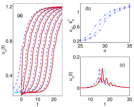
Figure 4: For $D=4$, $\gamma=2.2$, and $F=0.2$: (a) Compared time evolution of $w_{n}(t+\tau)$ (dot-dashed line) $w_{n}(t-\tau)$ (dashed line) and $u_{n}(t)$ (solid line) when $n=0,-1,-2,...$, (b) Compared profiles $u_{n}(T)$ (circles), $w_{n}(T\pm\tau)$ (asterisks), (c) Compared time evolution of $w_{n}^{\prime}(t\pm\tau)$ (dot-dashed and dashed lines) and $u_{n}^{\prime}(t)$ (solid line).

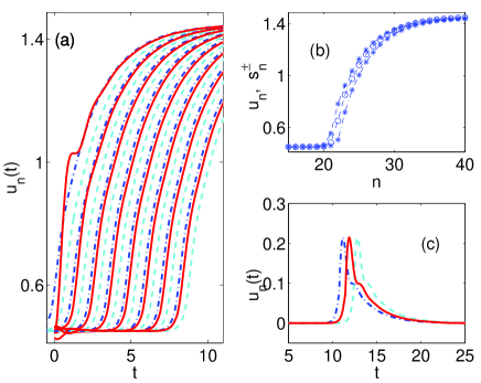
Figure 5: Same as Figure 4 when $F=0.45$.

III.2 Conservative dynamics

For small damping $\gamma^{2}\ll 4$, we know that the kink profiles develop oscillations in the trailing edge (see Figure 6) and that the Green functions oscillate and change sign (cf. Appendix B). However, $G_{nk}^{0}(t)$ and $G_{nk}^{1}(t)$ are positive for $0\leq t\leq T^{*}=T(\gamma,D)$. This critical time $T^{*}$ plays a key role for the stable propagation of waves. We will show in this section that kinks are stable provided $|c|>{1\over T^{*}}.$ Our argument does not say anything about the stability of kinks with lesser speeds. Moreover, $T^{*}\rightarrow 0$ and our lower bound on the wave front velocity tends to infinity, in the continuum limit.

We show in Appendix B that a rough estimate for $T^{*}$ is provided by ${2\pi\over\sqrt{4(1+4D)-\gamma^{2}}}$. For $\gamma=0$ and $D=4$, as chosen in our Figures (6)-(7), $T^{*}>1$. Then, kinks with $|c|>1$ are stable. In atk65 and wavy , stability was conjectured for speeds larger than the last minimum of $F(c)$, which is attained at $c_{cd}\sim 0.74$.

For small or zero damping we cannot use the previous comparison arguments because the trailing edge of the traveling wave front oscillates and monotonicity does not hold there. If we look at the traveling wave front profiles, it becomes clear that we should compare the monotone leading edges of the fronts. Figure 7 (a)-(b) depicts the trajectories $w_{n}(t)$ and their time derivatives $w_{n}^{\prime}(t)$ for a particular traveling wave front. We observe that $w_{n-1}(t)<w_{n}(t)<w_{n+1}(t)$ and $w_{n-1}^{\prime}(t)<w_{n}^{\prime}(t)<w_{n+1}^{\prime}(t)$ up to a certain time. Figure 7 (c) shows the initial configurations for $w_{n}(0)$ and the shifted waves $w_{n}(-\tau)$, $w_{n}(\tau)$. $w_{n}(0)$ is sandwiched between $w_{n}(-\tau)$ and $w_{n}(\tau)$ up to a point $n_{0}$. Figure 7 (d) depicts the initial velocity profiles $w_{n}^{\prime}(0)$, $w_{n}^{\prime}(-\tau)$ and $w_{n}^{\prime}(\tau)$. $w_{n}^{\prime}(0)$ is sandwiched between $w_{n}^{\prime}(-\tau)$ and $w_{n}^{\prime}(\tau)$ up to a point $n_{1}$. $n_{0}$ and $n_{1}$ mark the onset of the oscillatory tails. In general, $0\leq n_{0}\leq n_{1}$. As the wave advances, the ranges of $n$ for which $w_{n}(t-\tau)<w_{n}(t)=w(n-ct-{1\over 2})<w_{n}(t+\tau)$ change with $t$.

The main result of this section is the following stability theorem, whose proof can be found in Appendix D:

Theorem. Let us select the wave front profile so that $w_{n}(t)=w(n-ct-{1\over 2})$, with $c<0$ and $F>0$. Let $T^{*}$ be the maximum time up to which the Green functions $G_{nk}^{0}(t)$ and $G_{nk}^{1}(t)$ remain positive. We assume that the speed $|c|>{1\over T^{*}}$ and choose the initial states for (2), $u_{n}^{1}$ and $u_{n}^{0}$, in the set:

$$\begin{array}[]{ll}w_{n}(-\tau)<u_{n}^{0}<w_{n}(\tau),\;n\leq n_{0}\quad 0<\tau\ll{1\over 2|c|}\\ w_{n}^{\prime}(-\tau)<u_{n}^{1}<w_{n}^{\prime}(\tau),\;n\leq n_{1}\end{array}$$ (60)

$$\begin{array}[]{l}\sum_{n}|u_{n}^{0}-w_{n}(0)|<\epsilon,\quad\sum_{n}|u_{n}^{1}-w_{n}^{\prime}(0)|<\epsilon.\end{array}$$ (62)

for $\epsilon>0$ small and $\tau<\epsilon$. Then, we can find an increasing sequence of times $t_{k}$, $k=0,1,...$, with $t_{-1}=0$, such that:

$$\begin{array}[]{l}w_{n}(t-\tau)<u_{n}(t)<w_{n}(t+\tau),\quad n\leq n_{0}-k\\ w_{n}^{\prime}(t-\tau)<u_{n}^{\prime}(t)<w_{n}^{\prime}(t+\tau),\quad n\leq n_{1}-k\end{array}$$ (65)

for $t_{k-1}\leq t<t_{k}$. Furthermore, for $t>0$ and any $n$, we have:

$$|u_{n}(t)-w_{n}(t)|\leq\sum_{k}|G_{nk}^{1}(t)||u_{k}^{0}-w_{k}(0)|$$

$$+\sum_{k}|G_{n0}^{0}(t)||u_{k}^{1}-w_{k}^{\prime}(0)|+C(t)$$ (66)

$$C(t)=\sum_{k\leq 0,t\geq T_{k}-\tau}\int_{T_{k}-\tau}^{{\rm Min}(T_{k}+\tau,t)}G_{nk}^{0}(t-z)dz,$$

in which $T_{k}={k\over|c|}+{1\over 2|c|}$. Thus, the traveling wave front is stable when $\gamma=0$ or asymptotically stable when $\gamma>0$.

Let us clarify the meaning of (66). For $\gamma>0$, the sums $\sum_{k}|G_{nk}^{1}(t)|$, $\sum_{k}|G_{nk}^{0}(t)|$ decay exponentially with time. For small $\tau$, the function $|C(t)|\sim 2\tau\sum_{k\leq 0,t\geq T_{k}-\tau}|G_{nk}^{0}(t-T_{k})|$. This sum is finite and decays with time. This explains our asymptotical stability claim. When $\gamma=0$, the sums $\sum_{k}|G_{nk}^{1}(t)||u_{k}^{0}-w_{k}(0)|$, $\sum_{k}|G_{nk}^{0}(t)||u_{k}^{0}-w_{k}(0)|$ are bounded by a constant times ${\rm Max}_{k}|u_{k}^{0}-w_{k}(0)|+{\rm Max}_{k}|u_{k}^{0}-w_{k}(0)|.$ The function $|C(t)|$ is bounded by a constant times $\tau$ and is made small be choosing $\tau$ small. This explains our stability claim in the conservative case.

The inequalities (65) tell us that the leading edge of the propagating kink is sandwiched between the leading edges of the shifted traveling wave fronts $w_{n}(t+\tau)$ and $w_{n}(t-\tau)$. As the kink $u_{n}(t)$ advances, the times $t_{k}$ at which $u_{-k}(t)-{1\over 2}$ changes sign are bounded by the times at which the advanced and delayed wave fronts cross ${1\over 2}$: $T_{k}-\tau\leq t_{k}\leq T_{k}+\tau$. This fact is the key for obtaining the stability bound (66).

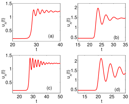
Figure 6: Trajectories $u_{n}(t)$ when $D=4$: (a) $\gamma=0.2$, $F=0.2$, (b) $\gamma=0.2$, $F=0.45$, (c) $\gamma=0.1$, $F=0.2$, (d) $\gamma=0.1$, $F=0.45$.

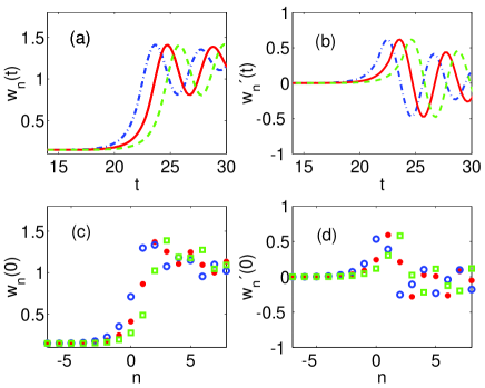
Figure 7: (a) Trajectories $w_{n-1}(t)$ (dash-dotted), $w_{n}(t)$ (solid), $w_{n+1}(t)$ (dashed); (b) same for $w_{n-1}^{\prime}(t)$, $w_{n}^{\prime}(t)$, $w_{n+1}(t)$; (c) initial configurations for $w_{n}(\tau)$ (circles), $w_{n}(0)$ (asterisks), $w_{n}(-\tau)$ (squares), the vertical line defines $n_{0}$; (d) same for $w_{n}^{\prime}(\tau)$, $w_{n}^{\prime}(0)$, $w_{n}^{\prime}(-\tau)$, the vertical lines defines $n_{1}$.

IV Coexistence

The results in Section III.2 indicate that stable static and traveling kinks may coexist. The only restriction on the traveling kinks is the monotonicity of the leading edge and a low bound on the speed. These conditions are satisfied by traveling wave fronts for a range of forces in which static wave fronts also exist. We show in this section how oscillating Green functions may force initial kink-like configurations (which would be pinned for large damping) to evolve into a traveling wave fronts provided the damping is small enough.

We fix $F<F_{cs}$ and select the static kink $s_{n}$ constructed in Section II for (2) with $s_{0}<{1\over 2}<s_{1}$. Let the initial condition for (2) be a piecewise constant profile: $u_{n}^{0}=F$ for $n\leq 0$, $u_{n}^{0}=1+F$ for $n\geq 1$ and $u_{n}^{1}=0$. Let $T^{*}$ the maximum time up to which $G_{nk}^{0}$ and $G_{nk}^{1}$ remain positive.

As long as $u_{n}(t)-{1\over 2}$ does not change sign for any $n$, $u_{n}(t)$ is given by formula (16) in Section II. We have $\sum_{k}G_{nk}^{0}(t)u_{k}^{1}\geq 0$ for $t\leq T^{*}$. Initially, $G_{nk}^{1}(t)$ is concentrated at $k=n$ and the sign of $\sum_{k}G_{nk}^{1}(t)(u_{k}^{0}-s_{k})$ is decided by the sign of $u_{n}^{0}-s_{n}$. If $u_{n}^{0}>s_{n}$, $u_{n}(t)\geq s_{n}$. In our case, this is true for $n\geq 1$. If $u_{n}^{0}<s_{n}$, $u_{n}(t)$ increases towards $s_{n}$ as $\sum_{k}G_{nk}^{1}(t)(u_{k}^{0}-s_{k})$ decays. By our choice of the initial state, $u_{0}(t)$ grows faster than the other components $u_{n}(t)$, $n<0$.

Now there are two possibilities depending on the value of the damping coefficients. For large damping, $G_{nk}^{1}(t)$ is positive for all times and $G_{nk}^{0}$ decays fast. Then $u_{0}(t)$ cannot surpass $s_{0}$. This initial data is pinned for large damping.

For small values of the damping, $G_{nk}^{1}(t)$ changes sign. Then $u_{0}(t)$ given by (16) may surpass $s_{0}$ and ${1\over 2}$ since the term $\sum_{k}G_{nk}^{1}(t)(u_{k}^{0}-s_{k})$ becomes positive for $t\geq T^{*}$. This process can be iterated to get a stably propagating wave, see Figure 1. A prediction for the speed is found in this way: it is the reciprocal of the time that $s_{0}+G_{00}^{1}(t)(F-s_{0})$ needs to reach ${1\over 2}$.

V More general potentials

We have focused our study on periodic piecewise parabolic potentials $V(u)={u^{2}\over 2}$, $|u|<{1\over 2}$. For these potentials, families of static and traveling wave fronts can be constructed analytically. Schmidt sch79 and later authors bre97 ; fla99 found exact monotone wave fronts of conservative systems by constructing models with nonlinearities such that the desired wave fronts were solutions of the models. For damped Frenkel-Kontorova or quartic double well potentials, stably propagating wave fronts have been found numerically wavy . Numerical studies of kink propagation in the conservative Frenkel-Kontorova model were carried out in pey84 .

The stability of propagating kinks in these models can be studied adapting the methods developed in this paper, but the analysis is technically more complicated preprint . For instance, taking $V(u)={u^{2}\over 2}$ for $|u|<{1\over 2}$, ${1\over 4}-{(u-1)^{2}\over 2}$ for $|u-1|<{1\over 2}$ we get a continuous piecewise linear source

$$g(s)=\left\{\begin{array}[]{ll}s\quad s<1/2\\ -s+{1\over 2}\quad{1\over 2}<s<3/2\\ s-1\quad s\geq 3/2\\ \end{array}\right.$$ (70)

The arguments in Sections III.1 and III.2 can be adapted by including new terms $\int_{0}^{t}\!\!\sum_{{1\over 2}<u_{k}<{3\over 2}}G_{nk}^{0}(t-z)(2u_{k}(z)-{1\over 2})dz$ in the integral expressions (105)-(108) and using that the function $h(s)=2s-1/2$ is increasing in $1/2<s<3/2$. Similarly, for a Frenkel-Kontorova potential, we write $g(s)=-as+(\sin(s)+as),a>0$. Then, we find the integral expression (82) with a nonlinear source $f_{k}=-\sin(u_{k})+au_{k}+F$, using the Green functions for the linear operator $u_{n}^{\prime\prime}+\gamma u_{n}^{\prime}-D(u_{n+1}-2u_{n}+u_{n-1})+au_{n}$. The parameter $a$ is chosen to ensure adequate monotonicity properties for $h(s)=-\sin(s)+as$ preprint .

VI Conclusions

We have developed a nonlinear stability theory for wave fronts in conservative and damped Frenkel-Kontorova models with piecewise linear sources based on integral formulations. Our results provide an analytical basis for the distinction between static and dynamic Peierls stresses, which arise as thresholds for the existence of stable static and traveling wave fronts. With little or zero damping, stable propagation of fronts is possible when their speeds surpass a critical value. The corresponding wave front profiles have a monotone leading edge, and, possibly, an oscillatory wake. Wave fronts can be oscillatory and yet stable. Whether slow wave fronts showing oscillations in the leading and trailing edges are stable remains an open question wavy . It is remarkable that high order quasicontinuum approximations such as those by Rosenau rosenau or by Boussinesq boussi have wave solutions comparable to the fast waves of the discrete conservative model truski .

Together with the stability theory we have presented an algorithm for the numerical computation of the dynamics of kinks. Our scheme has good stability properties and avoids distortions originated by artificial boundary conditions and time discretization.

Appendix A Green functions

We want to find an integral representation of the solution of the problem:

$$u_{n}^{\prime\prime}+\gamma u_{n}^{\prime}=D(u_{n+1}-2u_{n}+u_{n-1})-u_{n}+f_{n}$$ (71)

$$u_{n}(0)=u_{n}^{0},\quad u_{n}^{\prime}(0)=u_{n}^{1}$$ (72)

with $\gamma\geq 0,D>0$. Firstly, we get rid of the difference operator by using the generating functions $p(\theta,t)$, $f(\theta,t)$:

$$p(\theta,t)=\sum_{n}u_{n}(t)e^{-in\theta},\;f(\theta,t)=\sum_{n}f_{n}(t)e^{-in\theta}$$ (73)

Differentiating $p$ with respect to $t$ and using (71), we see that $p$ solves the ordinary differential equation:

$$p^{\prime\prime}(\theta,t)+\gamma p^{\prime}(\theta,t)+\omega(\theta)^{2}p(\theta,t)=f(\theta,t)$$ (74)

where $\omega(\theta)^{2}=1+4D\sin^{2}({\theta\over 2})$ and the obvious initial conditions for $p(\theta,t)$ follow from those for $u_{n}(t)$.

The solution $p$ depends on the roots of the polynomial $r^{2}+\gamma r+\omega(\theta)^{2}=0$. When ${\gamma^{2}\over 4}>\omega^{2}(\theta)$,

$$p(\theta,t)=p(\theta,0){e^{r_{-}(\theta)t}r_{+}(\theta)-e^{r_{+}(\theta)t}r_{-}(\theta)\over r_{+}(\theta)-r_{-}(\theta)}$$

$$+p^{\prime}(\theta,0){e^{r_{+}(\theta)t}-e^{r_{-}(\theta)t}\over r_{+}(\theta)-r_{-}(\theta)}$$

$$+\int_{0}^{t}{e^{r_{+}(\theta)(t-s)}-e^{r_{-}(\theta)(t-s)}\over r_{+}(\theta)-r_{-}(\theta)}f(\theta,s)ds$$ (75)

with $r_{\pm}(\theta)={-\gamma\pm\sqrt{\alpha(\theta)}\over 2}<0$ and $\alpha(\theta)=\gamma^{2}-4\omega(\theta)^{2}$. When ${\gamma^{2}\over 4}<\omega^{2}(\theta)$, the roots are complex:

$$p(\theta,t)=p(\theta,0)e^{{-\gamma\over 2}t}\Big{[}\cos\big{(}I(\theta)t\big{)}+{\gamma\sin\big{(}I(\theta)t\big{)}\over 2I(\theta)}\Big{]}$$

$$+p^{\prime}(\theta,0)\;e^{{-\gamma\over 2}t}{\sin\big{(}I(\theta)t\big{)}\over I(\theta)}$$

$$+\int_{0}^{t}e^{{-\gamma\over 2}(t-s)}{\sin\big{(}I(\theta)(t-s)\big{)}\over I(\theta)}f(\theta,s)ds$$ (76)

where $I(\theta)={\sqrt{-\alpha(\theta)}\over 2}$. When ${\gamma^{2}\over 4}=\omega^{2}(\theta),$

$$p(\theta,t)=p(\theta,0)e^{{-\gamma\over 2}t}(1+{\gamma\over 2}t)+p^{\prime}(\theta,0)\;e^{{-\gamma\over 2}t}t$$

$$+\int_{0}^{t}(t-s)e^{{-\gamma\over 2}(t-s)}f(\theta,s)ds$$ (77)

The solution $u_{n}(t)$ of (71) is recovered from the definition (73):

$$u_{n}(t)=\int_{-\pi}^{\pi}{d\theta\over 2\pi}e^{in\theta}p(\theta,t).$$ (78)

Here, $p(\theta,t)$ is defined by (75) when $\theta\in I_{1}$:

$$I_{1}=\{\theta\in[-\pi,\pi]\;|\;{\gamma^{2}\over 4}>\omega^{2}(\theta)\},$$ (79)

by (76) when $\theta\in I_{2}$:

$$I_{2}=\{\theta\in[-\pi,\pi]\;|\;{\gamma^{2}\over 4}<\omega^{2}(\theta)\}.$$ (80)

and by (77) when $\theta\in I_{3}$:

$$P=\{\theta\in[-\pi,\pi]\;|\;{\gamma^{2}\over 4}=\omega^{2}(\theta)\}.$$ (81)

Notice that $I_{1}=P=\emptyset$ if $\gamma^{2}<4$ and $I_{2}=P=\emptyset$ if $\gamma^{2}>4(1+4D)$. $P\neq\emptyset$ only if $4(1+4D)<\gamma^{2}<4$ and it then consists of two points.

Formula (78) can be rewritten as:

$$u_{n}(t)=\sum_{k}\big{[}G_{nk}^{0}(t)u_{k}^{\prime}(0)+G_{nk}^{1}(t)u_{k}(0)\big{]}$$

$$+\int_{0}^{t}\sum_{k}G_{nk}^{0}(t-s)f_{k}(s)ds$$ (82)

where

$$\begin{array}[]{l}G_{nk}^{0}(t)=\int_{-\pi}^{\pi}{d\theta\over 2\pi}e^{i(n-k)\theta}g^{0}(\theta,t)\\ G_{nk}^{1}(t)=\int_{-\pi}^{\pi}{d\theta\over 2\pi}e^{i(n-k)\theta}g^{1}(\theta,t)\end{array}$$ (85)

with

$$g^{0}(\theta,t)=\left\{\begin{array}[]{ll}{e^{r_{+}(\theta)t}-e^{r_{-}(\theta)t}\over r_{+}(\theta)-r_{-}(\theta)},\quad\theta\in I_{1}\\ e^{{-\gamma\over 2}t}t,\quad\theta\in P\\ e^{{-\gamma\over 2}t}{\sin\big{(}I(\theta)(t)\big{)}\over I(\theta)},\quad\theta\in I_{2}\end{array}\right.$$ (89)

$$g^{1}(\theta,t)=\left\{\begin{array}[]{ll}{e^{r_{-}(\theta)t}r_{+}(\theta)-e^{r_{+}(\theta)t}r_{-}(\theta)\over r_{+}(\theta)-r_{-}(\theta)},\quad\theta\in I_{1}\\ e^{{-\gamma\over 2}t}(1+{\gamma\over 2}t),\quad\theta\in P\\ e^{{-\gamma\over 2}t}\Big{[}\!\cos\big{(}I(\theta)t\big{)}\!+\!{\gamma\sin\big{(}I(\theta)t\big{)}\over 2I(\theta)}\!\Big{]},\;\theta\in I_{2}\end{array}\right.$$ (93)

For conservative chains, $\gamma=0$, $G_{nk}^{1}={dG_{nk}^{0}\over dt}$ and:

$$G_{nk}^{0}(t)=\int_{-\pi}^{\pi}{d\theta\over 2\pi}{e^{i(n-k)\theta}\over\omega(\theta)}\sin(\omega(\theta)t).$$ (94)

Green functions for hamiltonian chains were studied in bafalui and earlier in schrodinger . For overdamped chains, they were computed in fat98 .

Appendix B Properties of the Green functions

The Green functions for (71)-(72) have three relevant properties: they decay in time, they decay as $|n-k|\rightarrow\infty$ and are positive for some time. The property of spatial decay follows from integration by parts in (85):

$$\begin{array}[]{l}G_{nk}^{0}(t)={(-1)^{l}\over i^{l}(n-k)^{l}}\int_{-\pi}^{\pi}{d\theta\over 2\pi}e^{i(n-k)\theta}{\partial^{l}g^{0}(\theta,t)\over\partial\theta^{l}}\\ G_{nk}^{1}(t)={(-1)^{l}\over i^{l}(n-k)^{l}}\int_{-\pi}^{\pi}{d\theta\over 2\pi}e^{i(n-k)\theta}{\partial^{l}g^{1}(\theta,t)\over\partial\theta^{l}}\end{array}$$ (97)

when $n\neq k$. An immediate consequence is that $\sum_{k}|G_{nk}^{0}(t)|^{p}$ and $\sum_{k}|G_{nk}^{1}(t)|^{p}$ are finite for any $p\geq 1$. Therefore, we may obtain decay results as $|n|\rightarrow\infty$ for the solutions $u_{n}(t)$ of (71)-(72) given by (82) decay when the data $u_{n}^{0}$, $u_{n}^{1}$, $f_{n}(t)$ decay. Figures 8-9 illustrate the spatial decay of $G_{n}^{0}(t)=G_{n0}^{0}(t)$ and $G_{n}^{1}(t)=G_{n0}^{1}(t)$. Notice that, initially, both are concentrated about $n=0$.

Time decay and positivity depend on the strength of the damping. Let us start by the strongly damped case: $\gamma^{2}>4(1+4D)$. The Green functions are given by (85)-(93) with $I_{2}=P=\emptyset$:

• $G_{nk}^{0}(t)$ and $G_{nk}^{1}(t)$ are positive. The roots $r_{\pm}(\theta)$ being even with respect to $\theta$, both $G_{nk}^{0}(t)$ and $G_{nk}^{1}(t)$ are real and $e^{i(n-k)\theta}$ can be replaced by $\cos((n-k)\theta)$. The kernels $g_{0}(\theta,t)={e^{r_{+}(\theta)t}-e^{r_{-}(\theta)t}\over r_{+}(\theta)-r_{-}(\theta)}$ and $g_{1}(\theta,t)={e^{r_{-}(\theta)t}r_{+}(\theta)-e^{r_{+}(\theta)t}r_{-}(\theta)\over r_{+}(\theta)-r_{-}(\theta)}$ are even, positive, reach their maximum values at $\theta=0$ and decay as $\theta$ increases to $\pi$. The dominant contribution to the integrals (85) comes from a neighbourhood centered at $\theta=0$, where the oscillatory multiplier $\cos((n-k)\theta)$ is positive. Thus, both $G_{nk}^{0}(t)$ and $G_{nk}^{1}(t)$ are positive. Figure 8 illustrates their evolution as time grows. Notice the resemblance with the time evolution of heat kernels.

• $G_{nk}^{0}(t)$ and $G_{nk}^{1}(t)$ are bounded uniformly in $n,k$ by decaying exponentials in time:

  $$\begin{array}[]{l}|G_{nk}^{0}(t)|\leq{e^{r_{+}(0)t}-e^{r_{-}(\pi)t}\over\sqrt{\gamma^{2}-4(1+4D)}}\\ |G_{nk}^{1}(t)|\leq{e^{r_{-}(\pi)t}r_{+}(\pi)-e^{r_{+}(0)t}r_{-}(0)\over\sqrt{\gamma^{2}-4(1+4D)}}\end{array}$$ (100)

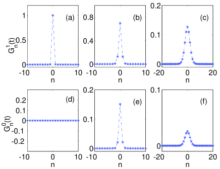
Figure 8: Time evolution of the Green functions for $D=4$ and $\gamma=10$: (a) $t=0$, (b) $t=0.5$, (c) $t=5$; (d) $t=0$, (e) $t=0.5$, (f) $t=5$.

We come now to intermediate damping $4<\gamma^{2}<4(1+4D)$. In this case both $I_{1}$ and $I_{2}$ are non empty. The piecewise defined kernels $g_{0}$ and $g_{1}$ are still even, take the largest values near zero (in $I_{1}$) and the smallest near $\pi$ (in $I_{2}$). The dominant contribution to $G_{nk}^{0}(t)$ and $G_{nk}^{1}(t)$ comes thus from $I_{1}$ and is positive. This is helped by the fact that the contribution coming from $I_{2}$ is initially positive and the factor $e^{-{\gamma\over 2}t}$ in the oscillatory region $I_{2}$ decays faster than the factor $e^{r_{+}(\theta)t}$ in the positive region $I_{1}$. Therefore, $G_{nk}^{0}(t)$ and $G_{nk}^{1}(t)$ are essentially positive in this intermediate regime, see Figure 9. This means that their large components are positive, despite the appearance of some negligible negative components. They can be roughly bounded by:

$$|G_{nk}^{0}(t)|\leq C_{0}e^{r_{+}(0)t},\;|G_{nk}^{1}(t)|\leq C_{1}e^{r_{+}(0)t}$$ (101)

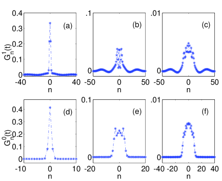
Figure 9: Time evolution of the Green functions for $D=4$ and $\gamma=2.2$: (a) and (d) $t=0.5$, (b) and (e) $t=2.5$, (c) and (f) $t=5$.

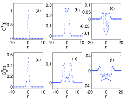
Figure 10: Time evolution of the Green functions for $D=4$ and $\gamma=1$: (a) $t=0$, (b) $t=0.5$, (c) $t=2.5$; (d) $t=0.5$, (e) $t=2.5$, (f) $t=5$.

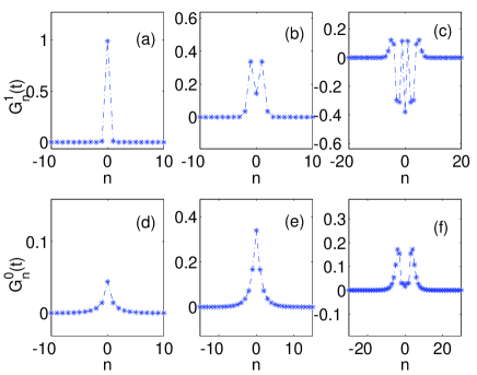
Figure 11: Time evolution of the Green functions for $D=4$ and $\gamma=0$: (a) and (d) $t=0.05$, (b) and (e) $t=0.5$, (c) and (f) $t=2.5$.

We address finally the weakly damped problems with $\gamma^{2}<4$. In this case, $I_{1}=P=\emptyset$. $G_{nk}^{0}(t)$ and $G_{nk}^{1}(t)$ are no longer globally positive. However, the kernels $g_{0}(\theta,t)$ and $g_{1}(\theta,t)$ are positive for $|t|<{2\pi\over\sqrt{4(1+4D)-\gamma^{2}}}=2T$ and $|t|<{\pi\over\sqrt{4(1+4D)-\gamma^{2}}}=T$, respectively. That means that $G_{nk}^{0}(t)>0$ and $G_{nk}^{1}(t)>0$ for $t$ in those intervals. They remain essentially positive in a larger interval. The kernels $g_{0}(\theta,t)$ and $g_{1}(\theta,t)$ become negative for $\theta$ near $\pi$ and remain positive for small $\theta$. This is enough for the relevant values of $G_{nk}^{1}(t)$ to remain positive up to a critical time $T^{*}$, often larger than $T$. We can get uniform bounds in time:

$$\begin{array}[]{l}|G_{nk}^{0}(t)|\leq{2\over\sqrt{4-\gamma^{2}}}e^{-{\gamma\over 2}t},\\ |G_{nk}^{1}(t)|\leq(1+{\gamma\over\sqrt{4-\gamma^{2}}})e^{-{\gamma\over 2}t}\end{array}$$ (104)

The same positivity properties and bounds are shared by the Green functions in the conservative case $\gamma=0$. Figures 10 and 11 illustrate the time evolution of the Green functions. A detailed study of the decay properties with respect to $n$ and $t$ for conservative problems can be found in bafalui .

Appendix C Stability of traveling wave fronts for strong damping

We now prove the stability theorem of Section III.1 for strong damping. The key idea of the proof is suggested by formula (10). When we solve (2) starting from different step-like initial states, we observe three types of terms in (10). The second and the third are increasing functions of the step-like configurations. The fourth term does not depend on the initial configuration. The first one can be made small by choosing a small velocity profile. Our proof proceeds in two steps. First, we establish a few properties of the traveling wave fronts. Second, we prove the stability bound (57).

Step 1: Basic properties of the traveling waves. For every $k$, we know that $w_{k}^{\prime}(t)>0$. Thus, each $w_{k}(t)$ crosses ${1\over 2}$ at a definite time $t_{k}$. Recall that we have selected the unique wave profile $w(x)$ satisfying $w(0)={1\over 2}$. Therefore, $w_{-k}(t)-{1\over 2}$ changes sign at time $T_{k}={k\over|c|}+{1\over 2|c|}>0$, $k=0,1,2,...$. For the shifted waves $w_{k}(t+\tau)$ and $w_{k}(t-\tau)$ the changes of sign take place at the shifted times $T_{k}^{+}=T_{k}-\tau$ and $T_{k}^{-}=T_{k}+\tau.$

The waves $w_{n}(t\pm\tau)$ solve the integral equation (10) with initial data $w_{n}(\pm\tau)$ and $w_{n}^{\prime}(\pm\tau).$ Using the times $T_{k}^{\pm}$, we can rewrite formula (10) in a more explicit form:

$$w_{n}(t\pm\tau)=\sum_{k}\Big{[}G_{nk}^{0}(t)w_{k}^{\prime}(\pm\tau)+G_{nk}^{1}w_{k}(\pm\tau)\Big{]}$$

$$+F\!\!\int_{0}^{t}\!\!\sum_{k}G_{nk}^{0}(t-z)dz+\!\!\int_{0}^{t}\!\sum_{k>0}G_{nk}^{0}(t-z)dz$$

$$+\sum_{k\leq 0}\int_{T_{k}^{\pm}}^{{\rm Max}(t,T_{k}^{\pm})}G_{nk}^{0}(t-z)dz$$ (105)

A term $\int_{T_{k}^{\pm}}^{t}G_{n,k}^{0}(t-z)dz$ is added whenever a factor $w_{k}(z\pm\tau)-{1\over 2}$ changes sign.

Step 2: Comparing $u_{n}(t)$ and $w_{n}(t\pm\tau)$. During the initial stage of the evolution of the chain $u_{0}(t)<{1\over 2}<u_{1}(t)$ and formula (10) reads:

$$\begin{array}[]{r}u_{n}(t)=\sum_{k}\Big{(}G_{nk}^{0}(t)u_{k}^{1}+G_{nk}^{1}(t)u_{k}^{0}\Big{)}+\\ \int_{0}^{t}\sum_{k>0}G_{nk}^{0}(t-z)dz+F\int_{0}^{t}\sum_{k}G_{nk}^{0}(t-z)dz\end{array}$$ (108)

By (53) and the positivity of $G_{nk}^{1}(t)$,

$$\sum_{k}\!\!G_{nk}^{1}(t)w_{k}(-\tau)\!<\!\!\sum_{k}\!\!G_{nk}^{1}(t)u_{k}^{0}\!<\!\!\sum_{k}\!\!G_{nk}^{1}(t)w_{k}(\tau).$$ (109)

By (56),

$$\begin{array}[]{l}\sum_{k}G_{nk}^{1}(t)\big{[}w_{k}(\tau)\!-\!u_{k}^{0}\big{]}\!+\!G_{nk}^{0}(t)\big{[}w_{k}^{\prime}(\tau)\!-\!u_{k}^{1}\big{]}>0\\ \sum_{k}G_{nk}^{1}(t)\big{[}u_{k}^{0}\!-\!w_{k}(-\tau)\big{]}\!+\!G_{nk}^{0}(t)\big{[}u_{k}^{1}\!-\!w_{k}^{\prime}(-\tau)\big{]}>0\end{array}$$ (112)

Therefore, (105)-(112) imply

$$w_{n}(t-\tau)<u_{n}(t)<w_{n}(t+\tau),$$ (113)

for all $n$ and $t\leq T_{0}^{+}$. Recall that $T_{0}^{+}\leq T_{0}^{-}$ by definition. Afterwards, $w_{0}(t+\tau)$ has crossed ${1\over 2}$ and $\int_{T_{0}^{+}}^{t}G_{n0}^{0}(t-z)dz>0$ must be added in the expression for $w_{n}(t+\tau)$. The ordering (113) still holds. At time $T_{0}^{-}$, $w_{0}(t-\tau)$ crosses ${1\over 2}$. By (112), $u_{0}(t)$ must cross before, at a time $t_{0}$.

In this way, we obtain a sequence of times $t_{k}$ at which $u_{-k}(t)-{1\over 2}$, changes sign satisfying $T_{k}^{+}<t_{k}<T_{k}^{-}$, $k=0,1,2,...$. Then,

$$u_{n}(t)=\sum_{k}\Big{[}G_{nk}^{0}(t)u_{k}^{1}+G_{nk}^{1}(t)u_{k}^{0}\Big{]}+$$

$$F\int_{0}^{t}\!\!\sum_{k}G_{nk}^{0}(t-z)dz+\!\!\int_{0}^{t}\!\sum_{k>0}G_{nk}^{0}(t-z)dz$$

$$+\sum_{k\leq 0}\int_{t_{k}}^{{\rm Max}(t,t_{k})}G_{nk}^{0}(t-z)dz$$ (114)

and (113) holds for all $t$. Our stability claim is proved.

Appendix D Stability of traveling wave fronts for conservative dynamics

In this section, we prove the stability theorem of Section III.2 for small or zero damping. The notation is the same as in Appendix C and the proof is organized in two steps.

Step 1: Initial stage. We compare $u_{n}(t)$ given by (108) with the shifted waves $w_{n}(t\pm\tau)$ given by (105), whereas $u_{n}^{\prime}(t)$ is compared with $w_{n}^{\prime}(t\pm\tau)$. The time derivatives are calculated by differentiating (105)-(108). Notice that ${dG_{nk}^{0}(t)\over dt}>0$ for small damping when $t\leq T^{*}$. Up to a first critical time $T_{0}^{+}$, $u_{k}(t)-{1\over 2}$ and $w_{k}(t\pm\tau)-{1\over 2}$ keep their sign for all $k$. Therefore,

$$\begin{array}[]{l}w_{n}(t\!-\!\tau\!)\!<\!u_{n}(t)\!<\!w_{n}(t\!+\!\tau\!),\;n\leq n_{0},\\ w_{n}^{\prime}(t\!-\!\tau\!)\!<\!u_{n}^{\prime}(t)\!<\!w_{n}^{\prime}(t\!+\!\tau\!),\;n\leq n_{1},\end{array}$$ (117)

for $t\leq T_{0}^{+}$. Recall that, initially, $G_{nk}^{1}$ and $G_{nk}^{0}$, together with their derivatives, take on their maximum values for $k$ close to $n$. This fact and (57)-(60) imply:

$$\begin{array}[]{l}w_{n}(t-\tau)<u_{n}(t)<w_{n}(t+\tau),\;n\leq n_{0}-1,\\ w_{n}^{\prime}(t-\tau)<u_{n}^{\prime}(t)<w_{n}^{\prime}(t+\tau),\;n\leq n_{1}-1,\end{array}$$ (120)

for $T_{0}^{+}\leq t\leq T_{1}^{+}$, choosing $\tau<T^{*}-T_{0}.$ This means that $u_{0}(t)-{1\over 2}$ changes sign at a time $t_{0}$ such that $T_{0}^{+}<t_{0}<T_{0}^{-}<T_{1}^{+}$. We then obtain formula (114) for $u_{n}(t)$ restricted to $t\leq T_{1}^{+}$. By subtracting (105) from (114), we find:

$$\begin{array}[]{r}\sum_{n}|u_{n}-w_{n}|(t)\leq\sum_{n}|G_{n0}^{1}(t)|\sum_{n}|u_{n}-w_{n}|(0)\\ +\sum_{n}|G_{n0}^{0}(t)|\sum_{n}|u_{n}^{\prime}-w_{n}^{\prime}|(0)+C(t)\end{array}$$ (123)

where

$$C(t)=\left\{\begin{array}[]{ll}0,&t\leq T_{0}^{+},\\ \int_{T_{0}^{+}}^{T_{0}^{-}}G_{n0}^{0}(t-z)dz,&t>T_{0}^{+},\end{array}\right.$$ (126)

and

$$\begin{array}[]{r}\sum_{n}|u_{n}^{\prime}-w_{n}^{\prime}|(t)\leq\sum_{n}|{dG_{n0}^{1}\over dt}(t)|\sum_{n}|u_{n}-w_{n}|(0)\\ +\sum_{n}|{dG_{n0}^{0}\over dt}(t)|\sum_{n}|u_{n}^{\prime}-w_{n}^{\prime}|(0)+R(t),\end{array}$$ (129)

where

$$R(t)=\left\{\begin{array}[]{ll}0,&t\leq T_{0}^{+},\\ \int_{T_{0}^{+}}^{T_{0}^{-}}{dG_{n0}^{0}\over dt}(t-z)dz,&t>T_{0}^{+},\end{array}\right.$$ (132)

for $t\leq T_{1}^{+}$. Let $S_{1}={\rm Max}_{[0,\infty)}\sum_{n}|G_{n0}^{1}(t)|$, $S_{2}={\rm Max}_{[0,\infty)}\sum_{n}|G_{n0}^{0}(t)|$, $S_{3}={\rm Max}_{[0,\infty)}\sum_{n}|{dG_{n0}^{1}\over dt}(t)|$ and $S_{4}={\rm Max}_{[0,\infty)}\sum_{n}|{dG_{n0}^{0}\over dt}(t)|$. Then, for $t\leq T_{1}^{+}$,

$$\begin{array}[]{l}\sum_{n}|u_{n}(t)-w_{n}(t)|\leq(S_{1}+S_{2})\varepsilon+2\tau|G_{n0}^{0}(T_{0})|,\\ \sum_{n}|u_{n}^{\prime}(t)-w_{n}^{\prime}(t)|\leq(S_{3}+S_{4})\varepsilon+2\tau|{dG_{n0}^{0}\over dt}(T_{0})|.\end{array}$$ (135)

The distances $|u_{n}(t)-w_{n}(t)|$, $|u_{n}^{\prime}(t)-w_{n}^{\prime}(t)|$ remain of order $\varepsilon$. In particular, the oscillatory tail of $u_{n}(t)$ for $n>n_{0}$ is contained in the same band that contains $w_{n}(t)$ for $n>n_{0}$.

Step 2: Generic stage. We iterate Step 1 starting at times $T_{l}^{+}$, $l=1,2,...,$ according to the following induction procedure. For a fixed $T_{l}^{+}$, (120) holds for $n<n_{0}-l$, $n<n_{1}-l$, $T_{l-1}^{+}\leq t\leq T_{l}^{+}$ and:

$$\begin{array}[]{l}\sum_{n}|u_{n}(t)-w_{n}(t)|\leq(S_{1}+S_{2})\varepsilon+2\tau S,\\ \sum_{n}|u_{n}^{\prime}(t)-w_{n}^{\prime}(t)|\leq(S_{3}+S_{4})\varepsilon+2\tau S\end{array}$$ (138)

holds for $t\leq T_{l}^{+}$, with $S={\rm Max}\big{(}\sum_{k}|G_{nk}^{0}(T_{k})|,$ $\sum_{k}|{dG_{nk}^{0}\over dt}(T_{k})|\big{)}.$ Now, we shall show that these properties also hold for $T_{l+1}^{+}$.

For $T_{l}^{+}\leq t\leq T_{l+1}^{+}$, the evolution of $w_{n}(t\pm\tau)$ and $u_{n}(t)$ is given by:

$$\begin{array}[]{l}w_{n}(t\pm\tau)=\sum_{k}G_{nk}^{0}(t-T_{l}^{+})w_{k}^{\prime}(T_{l}^{+}\pm\tau)+\\ \sum_{k}G_{nk}^{1}(t-T_{l}^{+})w_{k}(T_{l}^{+}\pm\tau)+\\ F\int_{T_{l-1}^{-}}^{t}\sum_{k}G_{nk}^{0}(t-z)dz+\\ \int_{T_{l}^{+}}^{t}\sum_{k>-l}G_{nk}^{0}(t-z)dz+\\ \sum_{k\leq-l}\int_{T_{k}^{\pm}}^{{\rm Max}(t,T_{k}^{\pm})}G_{nk}^{0}(t-z)dz\end{array}$$ (144)

$$\begin{array}[]{l}u_{n}(t)=\sum_{k}G_{nk}^{0}(t-T_{l}^{+})u_{k}^{\prime}(T_{l}^{+})+\\ \sum_{k}G_{nk}^{1}(t-T_{l}^{+})u_{k}(T_{l}^{+})+\\ F\int_{T_{l}^{+}}^{t}\!\!\sum_{k}G_{nk}^{0}(t-z)dz+\\ \!\!\int_{T_{l}^{+}}^{t}\!\sum_{k>-l}G_{nk}^{0}(t-z)dz+\\ \sum_{k\leq-l}\int_{T_{l}^{+}}^{t}G_{nk}^{0}(t-z)H(u_{k}(z)-{1\over 2})dz.\end{array}$$ (150)

Notice that we have taken as initial data the values of $w_{n}(t\pm\tau)$ and $u_{n}(t)$ at time $T_{l}^{+}$. In this way, formulae (144) and (150) only involve the values of the Green functions in a short time interval $[0,{1\over|c|}+2\tau]$. Since ${1\over|c|}+2\tau>T^{*}$, the Green functions are both positive. Recall that for this short time interval $G_{nk}^{1}$ and $G_{nk}^{0}$, together with their derivatives, take on large values for $k$ close to $n$. We can then use (120) for $n<n_{0}-l,n<n_{1}-l$ at time $T_{l}^{+}$, (138) and (144)-(150) to obtain (120) for $n<n_{0}-(l+1),n<n_{1}-(l+1)$ and $T_{l}^{+}\leq t\leq T_{l+1}^{+}$. This means that $u_{-l}(t)-{1\over 2}$ changes sign at a time $t_{l}$ such that $T_{l}^{+}<t_{l}<T_{l}^{-}<T_{l+1}^{+}$. We then obtain formula (114) for $u_{n}(t)$ restricted to $t\leq T_{l+1}^{+}$. Subtracting (105) from (114) for $t\leq T_{l+1}^{+}$, we find:

$$\begin{array}[]{l}\sum_{n}|u_{n}-w_{n}|(t)\leq(S_{1}+S_{2})\varepsilon+2\tau\sum_{k\leq l}|G_{nk}^{0}(T_{k})|\\ \sum_{n}|u_{n}^{\prime}-w_{n}^{\prime}|(t)\leq(S_{3}+S_{4})\varepsilon+2\tau\sum_{k\leq l}|{dG_{nk}^{0}\over dt}(T_{k})|\end{array}$$ (153)

This implies (138) for $t\leq T_{l+1}^{+}$. We are now ready to repeat the process starting at time $T_{l+1}^{+}$.

Step 3: Conclusion. From Step 2 we obtain a sequence of times $t_{l}$ for $l=1,2,...$, with $T_{l}^{+}<t_{l}<T_{l}^{-}$, at which $u_{-l}(t)-{1\over 2}$ changes sign. In this way, we keep track of the times $t_{l}$ at which changes of sign take place and obtain formula (114) for $u_{n}(t)$ for all $t$. Subtracting (105) from (114) we find the bound (66) on $|u_{n}-w_{n}|$.

References

- (1) E-address ana-carpio@mat.ucm.es.
- (2) J. Frenkel and T. Kontorova, J. Phys. USSR, 13, 1 (1938). O.M. Braun and Yu.S. Kivshar, Phys. Rep. 306, 1 (1998).
- (3) F.R.N. Nabarro, Theory of Crystal Dislocations (Oxford University Press, Oxford, UK, 1967).
- (4) L.I. Slepyan, Sov. Phys. Dokl. 26, 538 (1981).
- (5) P. M. Chaikin and T. C. Lubensky, Principles of condensed matter physics (Cambridge University Press, Cambridge, 1995). Chapter 10.
- (6) L.L. Bonilla, J. Phys. Condensed Matter 14, R341 (2002).
- (7) A. Tonnelier A., Phys. Rev. E, 67, 036105, (2003). A. Anderson and B. Sleeman, Int. J. Bif. Chaos, 5, 63 (1995).
- (8) J.P. Keener and J. Sneyd, Mathematical Physiology (Springer, New York, 1998), Chapter 9.
- (9) R. Hobart, J. Appl. Phys. 36, 1948 (1965).
- (10) E. Gerde and M. Marder, Nature 413, 285 (2001). D.A. Kessler, Nature 413, 260 (2001).
- (11) A. Carpio, L.L. Bonilla, Phys. Rev. E., 67, 056621, (2003).
- (12) W. Atkinson and N. Cabrera, Phys. Rev. 138, A763 (1965).
- (13) O. Kresse, L. Truskinovsky, J. Mech. Phys. Solids 51, 1305, (2003).
- (14) G. Fáth, Physica D, 116, 176 (1998). A. Carpio and L.L. Bonilla, Phys. Rev. Lett. 86, 6034 (2001).
- (15) M. Peyrard and M.D. Kruskal, Physica D 14, 88 (1984).
- (16) A. Carpio, L. L. Bonilla, A. Wacker and E. Schöll, Phys. Rev. E 61, 4866 (2000).
- (17) A. Carpio, unpublished, 2003.
- (18) V.H. Schmidt, Phys. Rev. B 20, 4397 (1979).
- (19) P.C. Bressloff and G. Rowlands, Physica D 106, 255 (1997).
- (20) S. Flach, Y. Zolotaryuk and K. Kladko, Phys. Rev. E 59, 6105 (1999).
- (21) P. Rosenau, Phys. Lett. A, 118 (5), 222, (1986).
- (22) M.J. Boussinesq, J. Math. Pures Appl. (Ser. 2) 17, 55, (1872).
- (23) J. Bafaluy, J.M. Rubi, Physica A, 153, 129, (1988), Physica A, 153, 147, (1988).
- (24) E. Schrodinger, Annalen der Physik, 44, 1053, (1914).