Statistical Theory of Magnetohydrodynamic Turbulence: Recent Results

Abstract

In this review article we will describe recent developments in statistical theory of magnetohydrodynamic (MHD) turbulence. Kraichnan and Iroshnikov first proposed a phenomenology of MHD turbulence where Alfvén time-scale dominates the dynamics, and the energy spectrum $E(k)$ is proportional to $k^{-3/2}$. In the last decade, many numerical simulations show that spectral index is closer to 5/3, which is Kolmogorov’s index for fluid turbulence. We review recent theoretical results based on anisotropy and Renormalization Groups which support Kolmogorov’s scaling for MHD turbulence.

Energy transfer among Fourier modes, energy flux, and shell-to-shell energy transfers are important quantities in MHD turbulence. We report recent numerical and field-theoretic results in this area. Role of these quantities in magnetic field amplification (dynamo) are also discussed. There are new insights into the role of magnetic helicity in turbulence evolution. Recent interesting results in intermittency, large-eddy simulations, and shell models of magnetohydrodynamics are also covered.

I Introduction

Fluid and plasma flows exhibit complex random behaviour at high Reynolds number; this phenomena is called turbulence. On the Earth this phenomena is seen in atmosphere, channel and rivers flows etc. In the universe, most of the astrophysical systems are turbulent. Some of the examples are solar wind, convective zone in stars, galactic plasma, accretion disk etc.

Reynolds number, defined as $UL/\nu$ ($U$ is the large-scale velocity, $L$ is the large length scale, and $\nu$ is the kinematic viscosity), has to be large (typically 2000 or more) for turbulence to set in. At large Reynolds number, there are many active modes which are nonlinearly coupled. These modes show random behaviour along with rich structures and long-range correlations. Presence of large number of modes and long-range correlations makes turbulence a very difficult problem that remains largely unsolved for more than hundred years.

Fortunately, random motion and presence of large number of modes make turbulence amenable to statistical analysis. Notice that the energy supplied at large-scales $(L)$ gets dissipated at small scales, say $l_{d}$. Experiments and numerical simulations show that the velocity difference $u(\mathbf{x+l})-u(\mathbf{x})$ has a universal probability density function (pdf) for $l_{d}\ll l\ll L$. That is, the pdf is independent of experimental conditions, forcing and dissipative mechanisms etc. Because of its universal behaviour, the above quantity has been of major interest among physicists for last sixty years. Unfortunately, we do not yet know how to derive the form of this pdf from the first principle, but some of the moments have been computed analytically. The range of scales $l$ satisfying $l_{d}\ll l\ll L$ is called inertial range.

In 1941 Kolmogorov K41a ; K41b ; K41c computed an exact expression for the third moment of velocity difference. He showed that under vanishing viscosity, third moment for velocity difference for homogeneous, isotropic, incompressible, and steady-state fluid turbulence is

$$\left\langle\left(u_{||}(\mathbf{x+l})-u_{||}(\mathbf{x})\right)^{3}\right\rangle=\frac{4}{5}\Pi l$$

where $||$ is the parallel component along $\mathbf{l}$, $\left\langle.\right\rangle$ stands for ensemble average, and $\Pi$ is the energy cascade rate, which is also equal to the energy supply rate at large scale $L$ and dissipation rate at the small scale $l_{d}$. Assuming fractal structure for the velocity field, and $\Pi$ to be constant for all $l$, we can show that the energy spectrum $E(k)$ is

$$E(k)=K_{Ko}\Pi^{2/3}k^{-5/3},$$

where $K_{Ko}$ is a universal constant, called Kolmogorov’s constant, and $L^{-1}\ll k\ll l_{d}^{-1}$. Numerical simulations and experiments verify the above energy spectrum apart from a small deviation called intermittency correction.

Physics of magnetohydrodynamic (MHD) turbulence is more complex than fluid turbulence. There are two coupled vector fields, velocity $\mathbf{u}$ and magnetic $\mathbf{b}$, and two dissipative parameters, viscosity and resistivity. In addition, we have mean magnetic field $B_{0}$ which cannot be transformed away (unlike mean velocity field which can be transformed away using Galilean transformation). The mean magnetic field makes the turbulence anisotropic, further complicating the problem. Availability of powerful computers and sophisticated theoretical tools have helped us understand several aspects of MHD turbulence. In the last ten years, there has been major advances in the understanding of energy spectra and fluxes of MHD turbulence. Some of these theories have been motivated by Kolmogorov’s theory for fluid turbulence. Note that incompressible turbulence is better understood than compressible turbulence. Therefore, our discussion on MHD turbulence is primarily for incompressible plasma. In this paper we focus on the universal statistical properties of MHD turbulence, which are valid in the inertial range. In this paper we will review the statistical properties of following quantities:

1. Inertial-range energy spectrum for MHD turbulence.

2. Various energy fluxes in MHD turbulence.

3. Energy transfers between various wavenumber shells.

4. Anisotropic effects of mean magnetic field.

5. Structure functions $<\left(u_{||}(\mathbf{x+l})-u_{||}(\mathbf{x})\right)^{n}>$ and $<\left(b_{||}(\mathbf{x+l})-b_{||}(\mathbf{x})\right)^{n}>$, where $u_{||}$ and $b_{||}$ are components of velocity and magnetic fields along vector $\mathbf{l}$.

6. Growth of magnetic field (dynamo).

Currently energy spectra and fluxes of isotropic MHD turbulence is quite well established, but anisotropy, intermittency, and dynamo is not yet fully understood. Therefore, items 1-3 will be discussed in greater detail.

Basic modes of incompressible MHD are Alfvén waves, which travel parallel and antiparallel to the mean magnetic field with speed $B_{0}$. The nonlinear terms induce interactions among these modes. In mid sixties Kraichnan Krai:65 and Iroshnikov Iros postulated that the time-scale for the nonlinear interaction is proportional to $B_{0}^{-1}$, leading to $E(k)\sim B_{0}^{1/2}k^{-3/2}$. However, research in last ten years Srid2 ; MKV:B0_RG ; Maro:Simulation ; ChoVish:localB show that the energy spectrum of MHD turbulence Kolmogorov-like ($k^{-5/3}$). Current understanding is that Alfvén waves are scattered by “local mean magnetic field” $B_{0}(k)\sim k^{-1/3}$, leading to Kolmogorov’s spectrum for MHD turbulence. The above ideas will be discussed in Sections VII and IX.

In MHD turbulence there are exchanges of energies among the velocity-velocity, velocity-magnetic, and magnetic-magnetic modes. These exchanges lead to energy fluxes from inside of the velocity/magnetic wavenumber sphere to the outside of the velocity/magnetic wavenumber sphere. Similarly we have shell-to-shell energy transfers in MHD turbulence. We have developed a new formalism called “mode-to-mode” energy transfer rates, using which we have computed energy fluxes and shell-to-shell energy transfers numerically and analytically Dar:flux ; MKV:MHD_PRE ; MKV:MHD_Flux ; MKV:MHD_Helical . The analytic calculations are based on field-theoretic techniques. Note that some of the fluxes and shell-to-shell energy transfers are possible only using “mode-to-mode” energy transfer, and cannot be computed using “combined energy transfer” in a triad Lesi:book .

Many analytic calculations in fluid and MHD turbulence have been done using field-theoretic techniques. Even though these methods are plagued with some inconsistencies, we get many meaningful results using them. In Sections VII, VIII, and IX we will review the field-theoretic calculations of energy spectrum, energy fluxes, and shell-to-shell energy transfers.

Growth of magnetic field in MHD turbulence (dynamo) is of central importance in MHD turbulence research. Earlier dynamo models (kinematic) assumed a given form of velocity field and computed the growth of large-scale magnetic field. These models do not take into account the back-reaction of magnetic field on the velocity field. In last ten years, many dynamic dynamo simulations have been done which also include the above mentioned back reaction. Role of magnetic helicity ($\mathbf{a}\cdot\mathbf{b}$, where $\mathbf{a}$ is the vector potential) in the growth of large-scale magnetic field is better understood now. Recently, Field et al. Fiel:Dynamo , Chou Chou:theo , Schekochihin et al. Maro:DynamoNlin and Blackman Blac:Rev_Dynamo have constructed theoretical dynamical models of dynamo, and studied nonlinear evolution and saturation mechanisms.

As mentioned above, pdf of velocity difference in fluid turbulence is still unsolved. We know from experiments and simulation that pdf is close to Gaussian for small $\delta u$, but is nongaussian for large $\delta u$. This phenomena is called intermittency. Note that various moments called Structure functions are connected to pdf. It can be shown that the structure functions are related to the “local energy cascade rate” $\Pi(k)$. Some phenomenological models, notably by She and Leveque SheLeve based on log-Poisson process, have been developed to compute $\Pi(k)$; these models quite successfully capture intermittency in both fluid and MHD turbulence. The predictions of these models are in good agreement with numerical results. We will discuss these issues in Section XI.

Numerical simulations have provided many important data and clues for understanding the dynamics of turbulence. They have motivated new models, and have verified/rejected existing models. In that sense, they have become another type of experiment, hence commonly termed as numerical experiments. Modern computers have made reasonably high resolution simulations possible. The highest resolution simulation in fluid turbulence is on $4096^{3}$ grid (e.g., by Gotoh Goto:DNS ), and in MHD turbulence is on $1024^{3}$ grid (e.g., by Haugen et al. Bran:Nonhelical_simulation ). Simulations of Biskamp Bisk:Kolm1 ; Bisk:Kolm2 , Cho et al. ChoVish:localB , Maron and Goldreich Maro:Simulation have verified 5/3 spectrum for MHD turbulence. Dar et al. Dar:flux have computed various energy fluxes in 2D MHD turbulence. Earlier, based on energy fluxes Verma et al. MKV:MHD_Simulation could conclude that Kolmogorov-like phenomenology models MHD turbulence better that Kraichnan and Iroshnikov’s phenomenology. Many interesting simulations have been done to simulate dynamo, e. g., Chou Chou:num and Brandenburg Bran:Alpha .

Because of large values of dissipative parameters, MHD turbulence requires large length and velocity scales. This make terrestrial experiments on MHD turbulence impossible. However, astrophysical plasmas are typically turbulent because of large length and velocity scales. Taking advantage of this fact, large amount of solar-wind in-situ data have been collected by spacecrafts. These data have been very useful in understanding the physics of MHD turbulence. In fact, in 1982 Matthaeus and Goldstein MattGold had shown that solar wind data favors Kolmogorov’s $k^{-5/3}$ spectrum over Kraichnan and Iroshnikov’s $k^{-3/2}$ spectrum. Solar wind data also shows that MHD turbulence exhibits intermittency. some of the observational results of solar wind will discussed in Section V. In addition to the above topics, we will also state the current results on the absolute equilibrium theories, decay of global quantities, two-dimensional turbulence, shell model of MHD turbulence, compressible turbulence etc.

Literature on MHD turbulence is quite extensive. Recent book “Magnetohydrodynamic Turbulence” by Biskamp BiskTurb:book covers most of the basics. MHD turbulence normally figures as one of the chapters in many books on Magnetohydrodynamics, namely Biskamp BiskNonl:book , Priest Prie:book , Raichoudhury Arna:book , Shu Shu:book , Cowling Cowl:book , Vedenov Vede:book . The recent developments are nicely covered by the review articles in an edited volume Pass:book . Some of the important review articles are by Montgomery Mont:SW , Pouquet Pouq:Rev , Krommes Krom:Rev_Intermittency ; Krom:Rev_Plasma . On dynamo, the key references are books by Moffatt Moff:book and Krause and Rädler Krau:book , and recent review articles Gilb:inbook ; Robe:Rev_Geo ; Bran:PR . Relatively, fluid turbulence has a larger volume of literature. Here we will list only some of the relevant ones. Leslie Lesl:book , McComb McCo:book ; McCo:rev ; McCo:RGBook , Zhou et al. ZhouMcCo:RGrev , and Smith and Woodruff Smit have reviewed field-theoretic treatment of fluid turbulence. The recent books by Frisch Fris:book and Lesieur Lesi:book cover recent developments and phenomenological theories. The review articles by Orszag Orsz:Rev , Kraichnan and Montgomery KraiMont , and Sreenivasan Sree:RMP are quite exhaustive.

In this review paper, we have focussed on statistical theory of MHD turbulence, specially on energy spectra, energy fluxes, and shell-to-shell energy transfers. These quantities have been analyzed analytically and numerically. A significant portion of the paper is devoted to self-consistent field-theoretic calculations of MHD turbulence and “mode-to-mode” energy transfer rates because of their power of analysis as well as our familiarity with these topics. These topics are new and are of current interest. Hence, this review article complements the earlier work. Universal laws are observed in the inertial range of homogeneous and isotropic turbulence. Following the similar approach, in analytic calculations of MHD turbulence, homogeneity and isotropy are assumed except in the presence of mean magnetic field.

To keep our discussion focussed, we have left out many important topics like coherent structures, astrophysical objects like accretion disks and Sun, transition to turbulence etc. Our discussion on compressible turbulence and intermittency is relatively brief because final word on these topics still awaited. Dynamo theory is only touched upon; the reader is referred to the above mentioned references for a detailed discussion. In the discussion on the solar wind, only a small number of results connected to energy spectra are covered.

The outline of the paper is as follows: Section II contains definition of various global and spectral quantities along with their governing equations. In Section III we discuss the formalism of “mode-to-mode” energy transfer rates in fluid and MHD turbulence. Using this formalism, formulas for energy fluxes and shell-to-shell energy transfer rates have been derived. Section IV contains the existing MHD turbulence phenomenologies which include Kraichnan’s 3/2 mode; Kolmogorov-like models of Goldreich and Sridhar. Absolute equilibrium theories and Selective decay are also discussed here. In Section V we review the observed energy spectra of the solar wind. Section VI describes Pseudo-spectral method along with the numerical results on energy spectra, fluxes, and shell-to-shell energy transfers. In these discussions we verify which of the turbulence phenomenologies are in agreement with the solar wind data and numerical results.

Next three sections cover applications of field-theoretic techniques to MHD turbulence. In Section VII we introduce Renormalization-group analysis of MHD turbulence, with an emphasis on the renormalization of “mean magnetic field” MKV:B0_RG , viscosity and resistivity MKV:MHD_RG . In Section VIII we compute various energy fluxes and shell-to-shell energy transfers in MHD turbulence using field-theoretic techniques. Here we also review eddy-damped quasi-normal Markovian (EDQNM) calculations of MHD turbulence. In Section IX we discuss the anisotropic turbulence calculations of Goldreich and Sridhar Srid1 ; Srid2 and Galtiers et al. Galt:Weak in significant details. The variations of turbulence properties with space dimensions have been discussed.

In Section X we briefly mention the main numerical and analytic results on homogeneous and isotropic dynamo. We include both kinematic and dynamic dynamo models, with emphasis being on the later. Section XI contains a brief discussion on intermittency models of fluid and MHD turbulence. Next section XII contains a brief discussion on the large-eddy simulations, decay of global energy, compressible turbulence, and shell model of MHD turbulence. Appendix A contains the definitions of Fourier series and transforms of fields in homogeneous turbulence. Appendix B and C contain the Feynman diagrams for MHD turbulence; these diagrams are used in the field-theoretic calculations. In the last Appendix D we briefly mention the main results of spectral theory of fluid turbulence in 2D and 3D.

II MHD: Definitions and Governing equations

II.1 MHD Approximations and Equations

MHD fluid is quasi-neutral, i.e., local charges of ions and electrons almost balance each other. The conductivity of MHD fluid is very high. As a consequence, the magnetic field lines are frozen, and the matter (ions and electrons) moves with the field. A slight imbalance in the motion creates electric currents, that in turn generates the magnetic field. The fluid approximation implies that the plasma is collisional, and the equations are written for the coarse-grained fluid volume (called fluid element) containing many ions and electrons. In the MHD picture, the ions (heavier particle) carry momentum, and the electrons (lighter particle) carry current. In the following discussion we will make the above arguments quantitative. In this paper we will use CGS units. For detailed discussions on MHD, refer to Cowling Cowl:book , Siscoe Sisc:book , and Shu Shu:book .

Consider MHD plasma contained in a volume. In the rest frame of the fluid element, the electric field $\mathbf{E^{\prime}=J}/\sigma$, where $\mathbf{J}$ is the electric current density, and $\sigma$ is the electrical conductivity. If $\mathbf{E}$ is the electric field in the laboratory frame, Lorenz transformation for nonrelativistic flows yields

$$\mathbf{E^{\prime}=E+\frac{u\times B}{\textrm{$c$}}=\frac{J}{\sigma},}$$ (1)

where $\mathbf{u}$ is the velocity of the fluid element, $\mathbf{B}$ is the magnetic field, and $c$ is the speed of light. Note that the current density, which is proportional to the relative velocity of electrons with relative to ions, remains unchanged under Galilean transformation. Since MHD fluid is highly conducting $(\sigma\rightarrow\infty)$,

$$E\approx\frac{u}{c}B.$$

This implies that for the nonrelativistic flows, $E\ll B$. Now let us look at one of the Maxwell’s equations

$$\nabla\times\mathbf{B}=\frac{4\pi}{c}\mathbf{J}+\frac{1}{c}\frac{\partial\mathbf{E}}{\partial t}.$$

The last term of the above equation is $(u/c)^{2}$ times smaller as compared to $\nabla\times\mathbf{B}$, hence it can be ignored. Therefore,

$$\mathbf{J}=\frac{c}{4\pi}\nabla\times\mathbf{B}.$$ (2)

Hence both $\mathbf{E}$ and $\mathbf{J}$ are dependent variables, and they can be written in terms of $\mathbf{B}$ and $\mathbf{u}$ as discussed above.

In MHD both magnetic and velocity fields are dynamic. To determine the magnetic field we make use of one of Maxwell’s equation

$$\frac{\partial\mathbf{B}}{\partial t}=-c\nabla\times\mathbf{E}.$$ (3)

An application of Eqs. (1,2) yields

$$\frac{\partial\mathbf{B}}{\partial t}=\nabla\times\left(\mathbf{u}\times\mathbf{B}\right)+\eta\nabla^{2}\mathbf{B},$$ (4)

or,

$$\frac{\partial\mathbf{B}}{\partial t}+(\mathbf{u}\cdot\nabla)\mathbf{B}=(\mathbf{B}\cdot\nabla)\mathbf{u}-\mathbf{B}\nabla\cdot\mathbf{u}+\eta\nabla^{2}\mathbf{B}.$$ (5)

The parameter $\eta$ is called the resistivity, and is equal to $c^{2}/(4\pi\sigma)$. The magnetic field obeys the following constraint:

$$\nabla\cdot\mathbf{B}=0.$$ (6)

The time evolution of the velocity field is given by the Navier-Stokes equation. In this paper, we work in an inertial frame of reference in which the mean flow speed is zero. This transformation is possible because of Galilean invariance. The Navier-Stokes equation is LandFlui:book ; Kund:book

$$\rho\left(\frac{\partial\mathbf{u}}{\partial t}+(\mathbf{u}\cdot\nabla)\mathbf{u}\right)=-\nabla p_{th}+\frac{1}{c}\mathbf{J\times B}+\mu\nabla^{2}\mathbf{u}+\frac{2\mu}{3}\nabla\nabla\cdot\mathbf{u},$$ (7)

where $\rho(\mathbf{x})$ is the density of the fluid, $p_{th}$ is the thermal pressure, and $\mu$ is the dynamic viscosity. Note that kinematic viscosity $\nu=\mu/\rho$. Substitution of $\mathbf{J}$ in terms of $\mathbf{B}$ [Eq. (2)] yields

$$\frac{\partial\mathbf{u}}{\partial t}+(\mathbf{u}\cdot\nabla)\mathbf{u}=\frac{1}{\rho}\left[-\nabla\left(p_{th}+\frac{B^{2}}{8\pi}\right)+(\mathbf{B}\cdot\nabla)\mathbf{B}\right]+\nu\nabla^{2}\mathbf{u}+\frac{2\nu}{3}\nabla\nabla\cdot\mathbf{u},$$ (8)

where $p_{th}+\frac{B^{2}}{8\pi}=p$ is called total pressure. The ratio $p_{th}/(B^{2}/8\pi)$ is called $\beta$, which describes the strength of the magnetic field with relative to thermal pressure.

Mass conservation yields the following equation for density field $\rho(\mathbf{x})$

$$\frac{\partial\rho}{\partial t}+\nabla\cdot\left(\rho\mathbf{u}\right)=0$$ (9)

Pressure can be computed from $\rho$ using equation of state

$$p=f\left(\rho\right)$$ (10)

This completes the basic equations of MHD, which are (5, 8, 9, 10). Using these equations we can determine the unknowns $(\mathbf{u,B,}\rho,p)$. Note that the number of equations and unknowns are the same.

When $\beta$ is high, $B^{2}$ is much less than $p_{th}$, and it can be ignored. On nondimensionalization of the Navier-Stokes equation, the term $\nabla p$ becomes $\left(d\rho/dx^{\prime}\right)/\rho$ $\times$$(C_{s}/U)^{2}$, where $C_{s}$ is the sound speed, $U$ is the typical velocity of the flow, $x^{\prime}$ is the position coordinate normalized with relative to the length scale of the system Trit:Book . $C_{s}\rightarrow\infty$ is the incompressible limit, which is widely studied because water, the most commonly found fluid on earth, is almost incompressible ($\delta\rho/\rho<$0.01) in most practical situations. The other limit $C_{s}\rightarrow 0$ or $U\gg C_{s}$ (supersonic) is the fully compressible limit, and it is described by Burgers equation. As we will see later, the energy spectrum for both these extreme limits well known. When $U/C_{s}\ll 1$ but nonzero, then we call the fluid to be nearly incompressible; Zank and Matthaeus Zank:Compress_PoF ; Zank:Compress_PRL have given theories for this limit. The energy and density spectra are not well understood for arbitrary $U/C_{s}$.

When $\beta$ is low, $p_{th}$ can be ignored. Now the Alfvén speed $C_{A}=B/\sqrt{4\pi\rho}$ plays the role of $C_{s}$. Hence, the fluid is incompressible if $U\ll C_{A}$ BiskTurb:book . For most part of this paper, we assume the magnetofluid to be incompressible. In many astrophysical and terrestrial situations (except shocks), incompressibility is a reasonably good approximation for the MHD plasma because typical velocity fluctuations are much smaller compared to the sound speed or the Alfvén speed. This assumption simplifies the calculations significantly. In Section XII.4 we will discuss the compressible MHD.

The incompressibility approximation can also be interpreted as the limit when volume of a fluid parcel will not change along its path, that is, $d\rho/dt=0$. From the continuity equation (9), the incompressibility condition reduces to

$$\nabla\cdot\mathbf{u}=0$$ (11)

This is a constraint on the velocity field u. Note that incompressibility does not imply constant density. However, for simplicity we take density to be constant and equal to 1. Under this condition, Eqs. (5, 8) reduce to

$$\frac{\partial\mathbf{u}}{\partial t}+(\mathbf{u}\cdot\nabla)\mathbf{u} = -\nabla p+(\mathbf{B}\cdot\nabla)\mathbf{B}+\nu\nabla^{2}\mathbf{u}$$ (12)

$$\frac{\partial\mathbf{B}}{\partial t}+(\mathbf{u}\cdot\nabla)\mathbf{B} = (\mathbf{B}\cdot\nabla)\mathbf{u}+\eta\nabla^{2}\mathbf{B}$$ (13)

To summarize, the incompressible MHD equations are

$\frac{\partial\mathbf{u}}{\partial t}+(\mathbf{u}\cdot\nabla)\mathbf{u}=-\nabla p+(\mathbf{B}\cdot\nabla)\mathbf{B}+\nu\nabla^{2}\mathbf{u}$

$\frac{\partial\mathbf{B}}{\partial t}+(\mathbf{u}\cdot\nabla)\mathbf{B}=(\mathbf{B}\cdot\nabla)\mathbf{u}+\eta\nabla^{2}\mathbf{B}$

$\nabla\cdot\mathbf{u}=0$

$\nabla\cdot\mathbf{B}=0$

When we take divergence of the equation Eq. (12), we obtain Poisson’s equation

$$-\nabla^{2}p=\nabla\cdot\left[(\mathbf{u}\cdot\nabla)\mathbf{u}-(\mathbf{B}\cdot\nabla)\mathbf{B}.\right]$$

Hence, given u and B fields at any given time, we can evaluate $p$. Hence $p$ is a dependent variable in the incompressible limit.

Incompressible MHD has two unknown vector fields $(\mathbf{u,B})$. They are determined using Eqs. (12, 13) under the constraints (6, 11). The fields $\mathbf{E},\mathbf{J}$ and $p$ are dependent variables that can be obtained in terms of $\mathbf{u}$ and $\mathbf{B}$.

The MHD equations are nonlinear, and that is the crux of the problem. There are two dissipative terms: viscous $(\nu\nabla^{2}\mathbf{u)}$ and resistive $(\eta\nabla^{2}\mathbf{B})$. The ratio of the nonlinear vs. viscous dissipative term is called Reynolds number $Re=UL/\nu$, where $U$ is the velocity scale, and $L$ is the length scale. There is another parameter called magnetic Reynolds number $Re_{m}=UL/\eta$. For turbulent flows, Reynolds number should be high, typically more than 2000 or so. The magnetic Prandtl number $\nu/\eta$ also plays an important role in MHD turbulence. Typical values of parameters in commonly studied MHD systems are given in Table 1 Encl ; Mont:SW ; MKV:SW_Nonclassical ; Kuls3 .

Table 1: Typical values of parameters in commonly studied MHD systems. Viscosity and resistivity of first 4 columns are rough estimates Encl ; Mont:SW ; MKV:SW_Nonclassical ; Kuls3

System	Earth’s Core	Solar Conve-ctive Zone	Solar Wind	Galactic Disk	Ioniz-ed H $(10^{5}K,42Pa)$	Hg
Length $(cm)$	$10^{8}$	$10^{10}$	$10^{13}$	$10^{22}$	$10$	$10$
Velocity $(cm/s)$	$10^{-2}$	$10^{4}$	$10^{6}$	$10^{6}$	$10^{2}$	$10$
Mean Mag. Field $(G)$	$10^{2}$	$10^{3}$	$10^{-5}$	$10^{-5}$	$10^{3}$	$10^{4}$
Density $(gm/cc)$	10	$10^{-5}$	$10^{-23}$	$10^{-24}$	$10^{-10}$	$10$
Kinematic viscosity $(cm^{2}/s)$	$10^{-2}$	$10^{11}$	$10^{4}$	$10^{21}$	$10^{5}$	$10^{-3}$
Reynolds Number	$10^{8}$	$10^{3}$	$10^{13}$	$10^{7}$	$10^{-2}$	$10^{5}$
Resistivity $(cm^{2}/s)$	$10^{4}$	$10^{11}$	$10^{4}$	$10^{7}$	$1.5\times 10^{5}$	$10^{4}$
Magnetic Reynolds no	$10^{2}$	$10^{3}$	$10^{4}$	$10^{21}$	$7\times 10^{-3}$	$10^{-2}$
Magnetic Prandtl no	$10^{-6}$	$1$	(1)?	$10^{14}$	0.7	$10^{-7}$

The calculation of viscosity and resistivity of MHD plasma is quite involved because of anisotropy caused by mean magnetic field Shu:book . In Table 1 we have provided rough estimates of these quantities.

II.2 Energy Equations and Conserved Quantities

In this subsection we derive energy equations for compressible and incompressible fluids. For compressible fluids we can construct equations for energy using Eqs. (5,8). Following Landau LandFlui:book we derive the following energy equation for the kinetic energy

$$\frac{\partial}{\partial t}\left(\frac{1}{2}\rho u^{2}+\rho\epsilon\right)=-\nabla\cdot\left[\left(\frac{1}{2}u^{2}+\epsilon\right)\rho\mathbf{u}\right]-\nabla\cdot p\mathbf{u}+\frac{1}{c}\mathbf{u}\cdot(\mathbf{J}\times\mathbf{B})+\Phi$$ (14)

where $\epsilon$ is the internal energy function. The first term in the RHS is the energy flux, and the second term is the work done by the pressure, which enhances the energy of the system. The third term in the RHS is work done by magnetic force on the fluid, while $\Phi$, a complex function of strain tensor, is the energy change due to surface forces.

For the evolution of magnetic energy we use Eq. (3) and obtain Kund:book

$$\frac{\partial}{\partial t}\frac{1}{8\pi}B^{2} = -\frac{c}{4\pi}\mathbf{B}\cdot\nabla\times\mathbf{E}$$ (15)

$$= -\nabla\cdot\frac{c}{4\pi}\mathbf{E}\times\mathbf{B}-\mathbf{J}\cdot\mathbf{E}$$

The first term in the RHS is the Poynting flux (energy flux of the electro-magnetic field), and the second term is the work done by the electro-magnetic field on fluid. The second term also includes the Joule dissipation term. Combination of Eqs. (14, 15) yields the following dynamical equation for the energy in MHD

$$\frac{\partial}{\partial t}\left(\frac{1}{2}\rho u^{2}+\rho\epsilon+\frac{1}{8\pi}B^{2}\right) = -\nabla\cdot\left[\left(\frac{1}{2}u^{2}+\epsilon\right)\rho\mathbf{u}+\frac{c}{4\pi}\mathbf{E}\times\mathbf{B}\right]$$

$$-\nabla\cdot p\mathbf{u}+\Phi+\frac{1}{\sigma}J^{2}$$

Here $\frac{1}{2}\rho u^{2}+\rho\epsilon+\frac{1}{8\pi}B^{2}$ is the total energy. Physical interpretation of the above equation is the following: the rate of change of total energy is the sum of energy flux, work done by pressure, and the viscous and resistive dissipation. It is convenient to use a new variable for magnetic field $B=B_{CGS}/\sqrt{4\pi}$. In terms of new variable, the total energy is $\frac{1}{2}\rho u^{2}+\rho\epsilon+\frac{1}{2}B^{2}$. From this point onward we use this new variable for magnetic field.

In the above equations we apply isoentropic and incompressibility conditions. For the incompressible fluids we can choose $\rho=1$. Landau LandFlui:book showed that under this condition $\epsilon$ is a constant. Hence, for incompressible MHD fluid we treat $(u^{2}+B^{2})/2$ as total energy. For ideal incompressible MHD ($\nu=\eta=0)$ the energy evolution equation is

$$\frac{\partial}{\partial t}\frac{1}{2}\left(u^{2}+B^{2}\right)=-\nabla\cdot\left[\left(\frac{1}{2}u^{2}+\frac{1}{2}B^{2}+p\right)\mathbf{u}\right]-2\nabla\cdot\left[\left(\mathbf{B}\cdot\mathbf{u}\right)\mathbf{B}\right]$$

By applying Gauss law we find that

$$\frac{\partial}{\partial t}\int\frac{1}{2}\left(u^{2}+B^{2}\right)d\mathbf{x}=-\oint\left[\left(\frac{1}{2}u^{2}+\frac{1}{2}B^{2}+p\right)\mathbf{u}+\left(\mathbf{B}\cdot\mathbf{u}\right)\mathbf{B}\right]\cdot d\mathbf{S}$$

For the boundary condition $B_{n}=u_{n}=0$ or periodic boundary condition, the total energy $\int$$1/2(u^{2}+B^{2})$ is conserved.

There are some more important quantities in MHD turbulence. They are listed in Table 2. Note that $\mathbf{A}$ is the vector potential and $\mathbf{\omega}$ is the vorticity field.

Table 2: Global Quantities in MHD

Quantity	Symbol	Definition	Conserved in MHD?
Kinetic Energy	$E^{u}$	$\int d\mathbf{x}u^{2}/2$	No
Magnetic Energy	$E^{B}$	$\int d\mathbf{x}B^{2}/2$	No
Total Energy	$E$	$\int d\mathbf{x}(u^{2}+B^{2})/2$	Yes (2D,3D)
Cross Helicity	$H_{c}$	$\int d\mathbf{x}(\mathbf{u}\cdot\mathbf{B})/2$	Yes (2D,3D)
Magnetic Helicity	$H_{M}$	$\int d\mathbf{x}(\mathbf{A}\cdot\mathbf{B})$/2	Yes (3D)
Kinetic Helicity	$H_{K}$	$\int d\mathbf{x}(\mathbf{u}\cdot\mathbf{\omega})/2$	No
Mean-square Vector Potential	$A2$	$\int d\mathbf{x}$$A^{2}/2$	Yes (2D)
Enstrophy	$\Omega$	$\int d\mathbf{x}\omega^{2}/2$	No

By following the same procedure described above, we can show that $E,H_{c},$ and $H_{M}$ are conserved in 3D MHD, while $E,H_{c}$ and $A2$ are conserved in 2D MHD MattGold ; BiskNonl:book . Note that in 3D fluids, $E^{u}$ and $H_{K}$ are conserved, while in 2D fluids, $E^{u}$ and $\Omega$ are conserved Lesl:book ; Lesi:book .

Magnetic helicity is a tricky quantity. Because of the choice of gauge it can be shown that magnetic helicity is not unique unless $B_{n}=0$ at the boundary. Magnetic helicity is connected with flux tubes, and plays important role in magnetic field generation. For details refer to Biskamp BiskNonl:book .

In addition to the above global quantities, there are infinite many conserved quantities. In the following we will show that the magnetic flux defined as

$$\Phi=\int\mathbf{B}\cdot d\mathbf{S},$$

where $d\mathbf{S}$ is the area enclosed by any closed contour moving with the plasma, is conserved. Since infinitely many closed curves are possible in any given volume, we have infinitely many conserved quantities. To prove the above conservation law, we use vector potential A, whose dynamical evolution is given by

$$\frac{\partial}{\partial t}\mathbf{A=u}\times\mathbf{B}+\nabla\phi,$$

where $\phi$ is the scalar potential MattGold . The above equation can be rewritten as

$$\frac{dA_{i}}{dt}=u_{k}\partial_{i}A_{k}+\partial_{i}\phi.$$

Now we write magnetic flux $\Phi$ in terms of vector potential

$$\Phi=\oint\mathbf{A}\cdot\mathbf{dl}.$$

The time derivative of $\Phi$ will be

$$\frac{d\Phi}{dt} = \oint\frac{dA_{i}}{dt}dl_{i}+A_{i}\frac{d}{dt}dl_{i}$$

$$= \oint d\phi+dl_{i}u_{k}\partial_{i}A_{k}+dl_{i}A_{k}\partial_{i}u_{k}$$

$$= 0$$

Hence, magnetic flux over any surface moving with the plasma is conserved.

The conserved quantities play very important role in turbulence. These aspects will be discussed later in Sections VII and VIII of this review. Now we turn to the linear solutions of MHD equations.

II.3 Linearized MHD Equations and their Solutions; MHD Waves

The fields can be separated into their mean and fluctuating parts: $\mathbf{B=B}_{0}+\mathbf{b}\textrm{ and }\rho=\rho_{0}+\delta\rho.$ Here $\mathbf{B}_{0}$ and $\rho_{0}$ denote the mean, and $\mathbf{b}$ and $\delta\rho$ denote the fluctuating fields. Note that the velocity field $\mathbf{u}$ is purely fluctuating field; its mean can be eliminated by Galilean transformation.

The linearized MHD equations are (cf. Eqs. [5, 8, 9])

$$\frac{\partial\mathbf{u}}{\partial t}-\left(\mathbf{B}_{0}\cdot\nabla\right)\mathbf{b} = -\frac{1}{\rho_{0}}\nabla p-\nabla\mathbf{B}_{0}\cdot\mathbf{b},$$

$$\frac{\partial\mathbf{b}}{\partial t}-\left(\mathbf{B}_{0}\cdot\nabla\right)\mathbf{u} = -\mathbf{B}_{0}\nabla\cdot\mathbf{u},$$

$$\frac{\partial\delta\rho}{\partial t}+\nabla\cdot\left(\rho_{0}\mathbf{u}\right) = 0.$$

We attempt a plane-wave solution for the above equations:

$$(\mathbf{u,b,}p,\delta\rho)=(\mathbf{u(k),b(k),}p(\mathbf{k)},\rho(\mathbf{k}))\exp\left(i\mathbf{k}\cdot\mathbf{x}-i\omega t\right).$$

Substitutions of these waves in the linearized equations yield

$$\omega\mathbf{u\left(\mathbf{k}\right)}+\left(\mathbf{B}_{0}.\mathbf{k}\right)\mathbf{b\left(\mathbf{k}\right)} = \frac{1}{\rho_{0}}\mathbf{k}p\left(\mathbf{k}\right)+\mathbf{k}\left(\mathbf{B}_{0}\cdot\mathbf{b}\right)$$

$$\omega\mathbf{b\left(\mathbf{k}\right)}+\left(\mathbf{B}_{0}.\mathbf{k}\right)\mathbf{u\left(\mathbf{k}\right)} = \mathbf{B}_{0}\left(\mathbf{k}\cdot\mathbf{u\left(\mathbf{k}\right)}\right)$$

$$\omega\rho\left(\mathbf{k}\right)-\rho_{0}\mathbf{k}\cdot\mathbf{u\left(\mathbf{k}\right)} = 0$$

Let us solve the above equations in coordinate system $(\mathbf{k},\mathbf{t}_{1},\mathbf{t_{2}})$ shown in Fig. 1. Here $\mathbf{t}_{1,2}$ are transverse to $\mathbf{k}$, with $\mathbf{t}_{1}$ in $\mathbf{B_{0}}$-$\mathbf{k}$ plane, and $\mathbf{t}_{2}$ perpendicular to this plane.

Figure 1: Basis vectors for MHD waves. Compressible waves have components along $\mathbf{k}$, while Alfvén waves have components along $\mathbf{t}_{1}$and $\mathbf{t}_{2}$.

The components of velocity and magnetic field along $\mathbf{t}_{1,2}$ are denoted by $u_{\perp}^{(1)},u_{\perp}^{(2)},b_{\perp}^{(1)},b_{\perp}^{(2)}$, and along $\mathbf{k}$ are $u_{||}$ and $b_{||}$. The angle between $\mathbf{B}_{0}$ and $\mathbf{k}$ is $\theta$. The equations along the new basis vectors are

$$\omega u_{||}-\frac{C_{s}^{2}}{\omega}k^{2}u_{||} = B_{0}b_{\perp}^{(1)}k\sin{\theta}$$ (16)

$$b_{||} = 0$$ (17)

$$\omega u_{\perp}^{(1)}+B_{0}k\cos{\theta}b_{\perp}^{(1)} = 0$$ (18)

$$\omega b_{\perp}^{(1)}+B_{0}k\cos{\theta}u_{\perp}^{(1)} = B_{0}k\sin{\theta}u_{||}$$ (19)

$$\omega u_{\perp}^{(2)}+B_{0}k\cos{\theta}b_{\perp}^{(2)} = 0$$ (20)

$$\omega b_{\perp}^{(2)}+B_{0}k\cos{\theta}u_{\perp}^{(2)} = 0$$ (21)

using $C_{s}=\sqrt{{p(k)/\rho(k)}}$. Note that $b_{||}=0$, which also follows from $\nabla\cdot\mathbf{b}=0$. From the above equations we can infer the following basic wave modes:

1. Alfvén wave (Incompressible Mode): Here $u_{||}=u_{\perp}^{(1)}=b_{\perp}^{(1)}=0$, and $u_{\perp}^{(2)}\neq 0,b_{\perp}^{(2)}\neq 0$, and the relevant equations are (20, 21). There are two solutions, which correspond to waves travelling antiparallel and parallel to the mean magnetic field with phase velocity $\pm C_{A}\cos{\theta}$ ($C_{A}=B_{0}$). For these waves thermal and magnetic pressures are constants. These waves are also called shear Alfvén waves.

2. Pseudo Alfvén wave (Incompressible Mode): Here $u_{||}=u_{\perp}^{(2)}=b_{\perp}^{(2)}=0$, and $u_{\perp}^{(1)}\neq 0,b_{\perp}^{(1)}\neq 0$, and the relevant equations are (18, 19). The two solutions correspond to waves moving antiparallel and parallel to the mean magnetic field with velocity $\pm C_{A}\cos{\theta}$.

3. Compressible Mode (Purely Fluid): Here $u_{\perp}^{(1)}=b_{\perp}^{(1)}=u_{\perp}^{(2)}=b_{\perp}^{(2)}=0$, and $u_{||}\neq 0$, and the relevant equation is (16). This is the sound wave in fluid arising due to the fluctuations of thermal pressure only.

4. MHD compressible Mode: Here $u_{\perp}^{(2)}=b_{\perp}^{(2)}=0$, and $u_{\perp}^{(1)}\neq 0,b_{\perp}^{(1)}\neq 0$, $u_{||}\neq 0$. Clearly, $u_{||}$ is coupled to $b_{\perp}^{(1)}$ as evident from Eqs. (16, 19). Solving Eqs. (16, 18, 19) yields

   $$\omega^{4}-\omega^{2}k^{2}\left(C_{s}^{2}+C_{A}^{2}\right)+C_{A}^{2}C_{S}^{2}k^{4}\cos^{2}{\theta}=0.$$

   Hence, the two compressible modes move with velocities

   $$V_{ph}^{2}=\frac{1}{2}\left[\left(C_{A}^{2}+C_{s}^{2}\right)\pm\sqrt{\left(C_{A}^{2}+C_{s}^{2}\right)^{2}-4C_{s}^{2}C_{A}^{2}\cos\theta}\right].$$ (22)

   The faster between the two is called fast wave, and the other one is called slow waves. The pressure variation for these waves are provided by both thermal and magnetic pressure. For details on these waves, refer to Sisco Sisc:book and Priest Prie:book .

Turbulent flow contains many interacting waves, and the solution cannot be written in a simple way. A popular approach to analyze the turbulent flows is to use statistical tools. We will describe below the application of statistical methods to turbulence.

II.4 Necessity for Statistical Theory of Turbulence

In turbulent fluid the field variables are typically random both in space and time. Hence the exact solutions given initial and boundary conditions will not be very useful even when they were available (they are not!). However statistical averages and probability distribution functions are reproducible in experiments under steady state, and they shed important light on the dynamics of turbulence. For this reason many researchers study turbulence statistically. The idea is to use the tools of statistical physics for understanding turbulence. Unfortunately, only systems at equilibrium or near equilibrium have been understood reasonably well, and a good understanding of nonequilibrium systems (turbulence being one of them) is still lacking.

The statistical description of turbulent flow starts by dividing the field variables into mean and fluctuating parts. Then we compute averages of various functions of fluctuating fields. There are three types are averages: ensemble, temporal, and spatial averages. Ensemble averages are computed by considering a large number of identical systems and taking averages at corresponding instants over all these systems. Clearly, ensemble averaging demands heavily in experiments and numerical simulations. So, we resort to temporal and/or spatial averaging. Temporal averages are computed by measuring the quantity of interest at a point over a long period and then averaging. Temporal averages make sense for steady flows. Spatial averages are computed by measuring the quantity of interest at various spatial points at a given time, and then averaging. Clearly, spatial averages are meaningful for homogeneous systems. Steady-state turbulent systems are generally assumed to be ergodic, for which the temporal average is equal to the ensemble average Fris:book .

As discussed above, certain symmetries like homogeneity help us in statistical description. Formally, homogeneity indicates that the average properties do not vary with absolute position in a particular direction, but depends only on the separation between points. For example, a homogeneous two-point correlation function is

$$\left\langle u_{i}(\mathbf{x},t)u_{j}(\mathbf{x^{\prime}},t)\right\rangle=C_{ij}(\mathbf{x-x^{\prime}},t)=C_{ij}(\mathbf{r},t).$$

Similarly, stationarity or steady-state implies that average properties depend on time difference, not on the absolute time. That is,

$$\left\langle u_{i}(\mathbf{x},t)u_{j}(\mathbf{x},t^{\prime})\right\rangle=C_{ij}(\mathbf{x},t-t^{\prime}).$$

Another important symmetry is isotropy. A system is said to be isotropic if its average properties are invariant under rotation. For isotropic systems

$$\left\langle u_{i}(\mathbf{x},t)u_{j}(\mathbf{x^{\prime}},t)\right\rangle=C_{ij}(\left|\mathbf{x-x^{\prime}}\right|,t)=C_{ij}(\left|\mathbf{r}\right|,t).$$

Isotropy reduces the number of independent correlation functions. Batchelor BatcTurb:book showed that the isotropic two-point correlation could be written as

$$C_{ij}(\mathbf{r})=C^{(1)}(r)r_{i}r_{j}+C^{(2)}(r)\delta_{ij}$$

where $C^{(1)}$ and $C^{(2)}$ are even functions of $r=|\mathbf{r}|.$ Hence we have reduced the independent correlation functions to two. For incompressible flows, there is only one independent correlation function BatcTurb:book .

In the previous subsection we studied the global conserved quantities. We revisit those quantities in presence of mean magnetic field. Note that mean flow velocity can be set to zero because of Galilean invariance, but the same trick cannot be used for the mean magnetic field. Matthaeus and Goldstein MattGold showed that the total energy and cross helicity formed using the fluctuating fields are conserved. We denote the fluctuating magnetic energy by $E^{b}$, in contrast to total magnetic energy $E^{B}$. The magnetic helicity $\int\mathbf{a}\cdot\mathbf{b}/2$ is not conserved, but $\mathbf{B}_{0}\cdot<\mathbf{A}>+\int\mathbf{a}\cdot\mathbf{b}/2$ instead is conserved.

In turbulent fluid, fluctuations of all scales exist. Therefore, it is quite convenient to use Fourier basis for the representation of turbulent fluid velocity and magnetic field. Note that in recent times another promising basis called wavelet is becoming popular. In this paper we focus our attention on Fourier expansion, which is the topic of the next subsection.

II.5 Turbulence Equations in Spectral Space

Turbulent fluid velocity $\mathbf{u}(\mathbf{x},t)$ is represented in Fourier space as

$$\mathbf{u}\left(\mathbf{x},t\right) = \int\frac{d\mathbf{k}}{(2\pi)^{d}}\mathbf{u}\left(\mathbf{k},t\right)\exp\left(i\mathbf{k\cdot x}\right)$$

$$\mathbf{u(}\mathbf{k},t) = \int d\mathbf{x}\mathbf{u}\left(\mathbf{x},t\right)\exp\left(-i\mathbf{k\cdot x}\right)$$

where $d$ is the space dimensionality.

In Fourier space, the equations for incompressible MHD are BiskTurb:book

$$\left(\frac{\partial}{\partial t}-i\left(\mathbf{B}_{0}\cdot\mathbf{k}\right)+\nu k^{2}\right)u_{i}(\mathbf{k},t) = -ik_{i}p_{tot}\left(\mathbf{k},t\right)-ik_{j}\int\frac{d\mathbf{p}}{(2\pi)^{d}}u_{j}(\mathbf{k-p},t)u_{i}(\mathbf{p},t)$$ (23)

$$+ik_{j}\int\frac{d\mathbf{p}}{(2\pi)^{d}}b_{j}(k-\mathbf{p},t)b_{i}(\mathbf{p},t),$$

$$\left(\frac{\partial}{\partial t}-i\left(\mathbf{B}_{0}\cdot\mathbf{k}\right)+\eta k^{2}\right)b_{i}(\mathbf{k},t) = -ik_{j}\int\frac{d\mathbf{p}}{(2\pi)^{d}}u_{j}(\mathbf{k-p},t)b_{i}(\mathbf{p},t)$$ (24)

$$+ik_{j}\int\frac{d\mathbf{p}}{(2\pi)^{d}}b_{j}(\mathbf{k-p},t)u_{i}(\mathbf{p},t),$$

with the following constrains

$$\mathbf{k}\cdot\mathbf{u\left(\mathbf{k}\right)} = 0,$$

$$\mathbf{k}\cdot\mathbf{b\left(\mathbf{k}\right)} = 0$$

The substitution of the incompressibility condition $\mathbf{k}\cdot\mathbf{u\left(\mathbf{k}\right)}=0$ into Eq. (23) yields the following expression for the pressure field

$$p\left(\mathbf{k}\right)=-\frac{k_{i}k_{j}}{k^{2}}\int\frac{d\mathbf{p}}{(2\pi)^{d}}\left[u_{j}(\mathbf{k-p},t)u_{i}(\mathbf{p},t)-b(\mathbf{k-p},t)b_{i}(\mathbf{p},t)\right].$$

Note that the density field has been taken to be a constant, and has been set equal to 1.

It is also customary to write the evolution equations symmetrically in terms of $\mathbf{p}$ and $\mathbf{k-p}$ variables. The symmetrized equations are

$$\left(\frac{\partial}{\partial t}-i\left(\mathbf{B}_{0}\cdot\mathbf{k}\right)+\nu k^{2}\right)u_{i}(\mathbf{k},t) = -\frac{i}{2}P_{ijm}^{+}(\mathbf{k})\int\frac{d\mathbf{p}}{(2\pi)^{d}}[u_{j}(\mathbf{p},t)u_{m}(\mathbf{k-p},t)$$ (25)

$$\hskip 85.35826pt-b_{j}(\mathbf{p},t)b_{m}(\mathbf{k-p},t)],$$

$$\left(\frac{\partial}{\partial t}-i\left(\mathbf{B}_{0}\cdot\mathbf{k}\right)+\eta k^{2}\right)b_{i}(\mathbf{k},t) = -iP_{ijm}^{-}(\mathbf{k})\int\frac{d\mathbf{p}}{(2\pi)^{d}}[u_{j}(\mathbf{p},t)b_{m}(\mathbf{k-p},t)],$$ (26)

where

$$P_{ijm}^{+}(\mathbf{k}) = k_{j}P_{im}(\mathbf{k})+k_{m}P_{ij}(\mathbf{k});$$

$$P_{im}(\mathbf{k}) = \delta_{im}-\frac{k_{i}k_{m}}{k^{2}};$$

$$P_{ijm}^{-}(\mathbf{k}) = k_{j}\delta_{im}-k_{m}\delta_{ij}.$$

Alfvén waves are fundamental modes of incompressible MHD. It turns out that the equations become more transparent when they are written in terms of Elsässer variables $\mathbf{z^{\pm}=u\pm b}$, which “represent” the amplitudes of Alfvénic fluctuations with positive and negative correlations. Note that no pure wave exist in turbulent medium, but the interactions can be conveniently written in terms of these variables. The MHD equations in terms of $\mathbf{z^{\pm}}$ are

$$\left(\frac{\partial}{\partial t}\mp i\left(\mathbf{B}_{0}\cdot\mathbf{k}\right)+\nu_{+}k^{2}\right)z_{i}^{\pm}(\mathbf{k})+\nu_{-}k^{2}z_{i}^{\mp}\left(\mathbf{k}\right) = -iM_{ijm}(\mathbf{k})\int d\mathbf{p}z_{j}^{\mp}(\mathbf{p})z_{m}^{\pm}(\mathbf{k-p}),$$ (27)

$$k_{i}z_{i}^{\pm}(\mathbf{k}) = 0,$$

where $\nu_{\pm}=(\nu\pm\eta)/2$ and

$$M_{ijm}(\mathbf{k})=k_{j}P_{im}(\mathbf{k}).$$

From the Eq. (27) it is clear that the interactions are between $\mathbf{z^{+}}$ and $\mathbf{z^{-}}$ modes.

Energy and other second-order quantities play important roles in MHD turbulence. For a homogeneous system these quantities are defined as

$$\left\langle X_{i}(\mathbf{k},t)Y_{j}(\mathbf{k^{\prime}},t)\right\rangle=C_{ij}^{XY}(\mathbf{k},t)(2\pi)^{d}\delta(\mathbf{k+k^{\prime}}),$$

where $\mathbf{X,Y}$ are vector fields representing $\mathbf{u}$, $\mathbf{b},$ or $\mathbf{z}^{\pm}$. The spectrum is also related to correlation function in real space

$$C_{ij}^{XY}(\mathbf{r})=\int\frac{d\mathbf{k}}{(2\pi)^{d}}C_{ij}^{XY}\left(\mathbf{k}\right)\exp\left(i\mathbf{k\cdot r}\right).$$

When mean magnetic field is absent, or its effects are ignored, then we can take $C_{ij}^{XY}(\mathbf{k})$ to be an isotropic tensor, and it can be written as BatcTurb:book

$$C_{ij}^{XY}(\mathbf{k})=P_{ij}(\mathbf{k})C^{XY}(k).$$ (28)

When turbulence is isotropic and $\mathbf{X=Y}$, then a quantity called 1D spectrum or reduced spectrum $E^{X}(k)$ defined below is very useful.

$$E^{X}=\frac{1}{2}\left\langle X^{2}\right\rangle =\frac{1}{2} \int\frac{d\mathbf{k}}{(2\pi)^{d}}C_{ii}^{XX}\left(\mathbf{k}\right)$$

$$\int E^{X}(k)dk = \frac{1}{2}\int dk\frac{S_{d}k^{d-1}}{(2\pi)^{d}}P_{ii}(\mathbf{k})C^{XX}\left(\mathbf{k}\right)$$

$$= \int dk\frac{S_{d}k^{d-1}(d-1)}{2(2\pi)^{d}}C^{XX}\left(\mathbf{k}\right),$$

where $S_{d}=2\pi^{d/2}/\Gamma{(d/2)}$ is the area of $d-$dimensional unit sphere. Therefore,

$$E^{X}(k)=C^{XX}(\mathbf{k})k^{d-1}\frac{S_{d}(d-1)}{2(2\pi)^{d}}.$$ (29)

Note that the above formula is valid only for isotropic turbulence. We have tabulated all the important spectra of MHD turbulence in Table 3. The vector potential $\mathbf{A=A_{0}+a}$, where $\mathbf{A_{0}}$ is the mean field, and $\mathbf{a}$ is the fluctuation.

Table 3: Various Spectra of MHD Turbulence

Quantity	Symbol	Derived from	Symbol for 1D
Kinetic energy spectrum	$C^{uu}\left(\mathbf{k}\right)$	$\left\langle u_{i}(\mathbf{k})u_{j}(\mathbf{k^{\prime}})\right\rangle$	$E^{u}$$\left(k\right)$
Magnetic energy spectrum	$C^{bb}$$\left(\mathbf{k}\right)$	$\left\langle b_{i}(\mathbf{k})b_{j}(\mathbf{k^{\prime}})\right\rangle$	$E^{b}\left(k\right)$
Total energy spectrum	$C$$\left(\mathbf{k}\right)$	$C^{uu}+C^{bb}$	$E$$\left(k\right)$
Cross helicity spectrum	$C^{ub}$$\left(\mathbf{k}\right)$	$\left\langle u_{i}(\mathbf{k})b_{j}(\mathbf{k^{\prime}})\right\rangle$	$H_{c}\left(k\right)$
Elsässer variable spectrum	$C^{\pm\pm}$$\left(\mathbf{k}\right)$	$\left\langle z_{i}^{\pm}(\mathbf{k})z_{j}^{\pm}(\mathbf{k^{\prime}})\right\rangle$	$E^{\pm}$$\left(k\right)$
Elsässer variable spectrum	$C^{\pm\mp}\left(\mathbf{k}\right)$	$\left\langle z_{i}^{\pm}(\mathbf{k})z_{j}^{\mp}(\mathbf{k^{\prime}})\right\rangle$	$E^{R}\left(k\right)$
Enstrophy spectrum	$\Omega\left(\mathbf{k}\right)$	$\left\langle\omega_{i}(\mathbf{k})\omega_{j}(\mathbf{k^{\prime}})\right\rangle$	$\Omega\left(k\right)$
Mean-square vector pot. spectrum	$A2$$\left(\mathbf{k}\right)$	$\left\langle a_{i}(\mathbf{k})a_{j}(\mathbf{k^{\prime}})\right\rangle$	$A2$$\left(k\right)$

The global quantities defined in Table 2 are related to the spectra defined in Table 3 by Perceval’s theorem BatcTurb:book . Since the fields are homogeneous, Fourier integrals are not well defined. In Appendix A we show that energy spectra defined using correlation functions are still meaningful because correlation functions vanish at large distances. We consider energy per unit volume, which are finite for homogeneous turbulence. As an example, the kinetic energy per unit volume is related to energy spectrum in the following manner:

$$\frac{1}{L^{d}}\int d\mathbf{x}\frac{1}{2}\left\langle u^{2}\right\rangle=\frac{1}{2}\int\frac{d\mathbf{k}}{(2\pi)^{d}}C_{ii}(\mathbf{k})=\int E^{u}(k)dk$$

Similar identities can be written for other fields.

In three dimensions we have two more important quantities, magnetic and kinetic helicities. In Fourier space magnetic helicity $H_{M}(\mathbf{k})$ is defined using

$$\left\langle a_{i}\left(\mathbf{k},t\right)b_{j}\left(\mathbf{k^{\prime}},t\right)\right\rangle=P_{ij}\left(\mathbf{k}\right)H_{M}(\mathbf{k})(2\pi)^{d}\delta(\mathbf{k+k^{\prime}})$$

The total magnetic helicity $H_{M}$ can be written in terms of

$$H_{M} = \frac{1}{2}\left\langle\mathbf{a}(\mathbf{x})\cdot\mathbf{b}(\mathbf{x})\right\rangle$$

$$=\frac{1}{2} \int\frac{d\mathbf{k}}{(2\pi)^{d}}\frac{d\mathbf{k^{\prime}}}{(2\pi)^{d}}\left\langle\mathbf{a}(\mathbf{k})\cdot\mathbf{b}(\mathbf{k^{\prime}})\right\rangle$$

$$= \int\frac{d\mathbf{k}}{(2\pi)^{d}}H_{M}(\mathbf{k})$$

$$= \int dkH_{M}(k)$$

Therefore, one dimensional magnetic helicity $H_{M}$ is

$$H_{M}(k)=\frac{4\pi k^{2}}{(2\pi)^{3}}H_{M}(\mathbf{k}).$$

Using the definition $\mathbf{b}(\mathbf{k})=i\mathbf{k}\times\mathbf{a}(\mathbf{k})$, we obtain

$$\left\langle b_{i}\left(\mathbf{k},t\right)b_{j}\left(\mathbf{k^{\prime}},t\right)\right\rangle=\left[P_{ij}\left(\mathbf{k}\right)C^{bb}(\mathbf{k})-i\epsilon_{ijl}k_{l}H_{M}(\mathbf{k})\right](2\pi)^{d}\delta(\mathbf{k+k^{\prime}})$$

The first term is the usual tensor described in Eq. (28), but the second term involving magnetic helicity is new. We illustrate the second term with an example. If $\mathbf{k}$ is along $z$ axis, then

$$b_{x}(\mathbf{k})b_{y}(\mathbf{k})=-ikH_{M}(\mathbf{k}).$$

This is a circularly polarized field where $b_{x}$ and $b_{y}$ differ by a phase shift of $\pi/2$. Note that the magnetic helicity breaks mirror symmetry.

A similar analysis for kinetic helicity shows that

$$\left\langle u_{i}\left(\mathbf{k},t\right)\Omega_{j}\left(\mathbf{k^{\prime}},t\right)\right\rangle=P_{ij}\left(\mathbf{k}\right)H_{K}(\mathbf{k})(2\pi)^{d}\delta(\mathbf{k+k^{\prime}})$$

$$H_{K}=\frac{1}{2}\left\langle\mathbf{u}\cdot\mathbf{\Omega}\right\rangle=\int\frac{d\mathbf{k}}{(2\pi)^{d}}H_{K}(\mathbf{k})$$

and

$$\left\langle u_{i}\left(\mathbf{k},t\right)u_{j}\left(\mathbf{k^{\prime}},t\right)\right\rangle=\left[P_{ij}\left(\mathbf{k}\right)C^{uu}(\mathbf{k})-i\epsilon_{ijl}k_{l}\frac{H_{M}(\mathbf{k})}{k^{2}}\right](2\pi)^{d}\delta(\mathbf{k+k^{\prime}}).$$

We can Fourier transform time as well using

$$\mathbf{u}\left(\mathbf{x},t\right) = \int d\hat{{k}}\mathbf{u}\left(\mathbf{k},\omega\right)\exp\left(i\mathbf{k\cdot x}-i\omega t\right)$$

$$\mathbf{u(}\mathbf{k},\omega) = \int d\mathbf{x}dt\mathbf{u}\left(\mathbf{x},t\right)\exp\left(-i\mathbf{k\cdot x}+i\omega t\right)$$

where $d\hat{{k}}=d\mathbf{k}d\omega/(2\pi)^{d+1}$. The resulting MHD equations in $\hat{{k}}=(\mathbf{k},\omega)$ space are

$$\left(-i\omega+\nu k^{2}\right)u_{i}(\hat{{k}}) = -\frac{i}{2}P_{ijm}^{+}({\textbf{k}})\int_{\hat{{p}}+\hat{{q}}=\hat{{k}}}d\hat{{p}}\left[u_{j}(\hat{{p}})u_{m}(\hat{{q}})-b_{j}(\hat{{p}})b_{m}(\hat{{q}})\right],$$ (30)

$$\left(-i\omega+\eta k^{2}\right)b_{i}(\hat{{k}}) = -iP_{ijm}^{-}({\textbf{k}})\int_{\hat{{p}}+\hat{{q}}=\hat{{k}}}d\hat{{p}}\left[u_{j}(\hat{{p}})b_{m}(\hat{{q}})\right],$$ (31)

or,

$$\left(-i\omega\mp i\left({\textbf{B}}_{0}\cdot{\textbf{k}}\right)+\nu_{+}k^{2}\right)z_{i}^{\pm}(\hat{k})+\nu_{-}k^{2}z_{i}^{\mp}(\hat{{k}})=-iM_{ijm}({\textbf{k}})\int d\hat{{p}}z_{j}^{\mp}(\hat{{p}})z_{m}^{\pm}(\hat{{k}}-\hat{{p}})$$ (32)

After we have introduced the energy spectra and other second-order correlation functions, we move on to discuss their evolution.

II.6 Energy Equations

The energy equation for general (compressible) Navier-Stokes is quite complex. However, incompressible Navier-Stokes and MHD equations are relatively simpler, and are discussed below.

From the evolution equations of fields, we can derive the following spectral evolution equations for incompressible MHD

$$\left(\frac{\partial}{\partial t}+2\nu k^{2}\right)C^{uu}\left(\mathbf{k},t\right) = \frac{2}{\left(d-1\right)\delta\left(\mathbf{k+k^{\prime}}\right)}\int_{\mathbf{k^{\prime}+p+q=0}}\frac{d\mathbf{p}}{(2\pi)^{2d}}[-\Im\left\langle\left(\mathbf{k^{\prime}}\cdot\mathbf{u(q)}\right)\left(\mathbf{u(p)}\cdot\mathbf{u(k^{\prime})}\right)\right\rangle$$ (33)

$$\hskip 85.35826pt+\Im\left\langle\left(\mathbf{k^{\prime}}\cdot\mathbf{b(q)}\right)\left(\mathbf{b(p)}\cdot\mathbf{u(k^{\prime})}\right)\right\rangle],$$

$$\left(\frac{\partial}{\partial t}+2\eta k^{2}\right)C^{bb}\left(\mathbf{k},t\right) = \frac{2}{\left(d-1\right)\delta\left(\mathbf{k+k^{\prime}}\right)}\int_{\mathbf{k^{\prime}+p+q=0}}\frac{d\mathbf{p}}{(2\pi)^{2d}}[-\Im\left\langle\left(\mathbf{k^{\prime}}\cdot\mathbf{u(q)}\right)\left(\mathbf{b(p)}\cdot\mathbf{b(k^{\prime})}\right)\right\rangle$$ (34)

$$\hskip 85.35826pt+\Im\left\langle\left(\mathbf{k^{\prime}}\cdot\mathbf{b(q)}\right)\left(\mathbf{u(p)}\cdot\mathbf{b(k^{\prime})}\right)\right\rangle],$$

where $\Im$ stands for the imaginary part. Note that $\mathbf{k^{\prime}+p+q=0}$ and $\mathbf{k^{\prime}=-k}$. In Eq. (33) the first term in the RHS provides the energy transfer from the velocity modes to $\mathbf{u(k)}$ mode, and the second term provides the energy transfer from the magnetic modes to $\mathbf{u(k)}$ mode. While in Eq. (34) the first term in the RHS provides the energy transfer from the magnetic modes to $\mathbf{b(k)}$ mode, and the second term provides the energy transfer from the velocity modes to $\mathbf{b(k)}$ mode. Note that pressure couples with compressible modes, hence it is absent in the incompressible equations. Simple algebraic manipulation shows that the mean magnetic field also disappears in the energy equation. In a finite box, using $\left\langle\left|\mathbf{u}(\mathbf{k})\right|^{2}\right\rangle=C(\mathbf{k})/((d-1)L^{d})$, and $\delta(\mathbf{k})(2\pi)^{d}=L^{d}$ (see Appendix A), we can show that

$$\left(\frac{\partial}{\partial t}+2\nu k^{2}\right)\frac{1}{2}\left\langle\left|\mathbf{u}(\mathbf{k})\right|^{2}\right\rangle = \sum[-\Im\left\langle\left(\mathbf{k^{\prime}}\cdot\mathbf{u(q)}\right)\left(\mathbf{u(p)}\cdot\mathbf{u(k^{\prime})}\right)\right\rangle+\Im\left\langle\left(\mathbf{k^{\prime}}\cdot\mathbf{b(q)}\right)\left(\mathbf{b(p)}\cdot\mathbf{u(k^{\prime})}\right)\right\rangle],$$

$$\left(\frac{\partial}{\partial t}+2\nu k^{2}\right)\frac{1}{2}\left\langle\left|\mathbf{b}(\mathbf{k})\right|^{2}\right\rangle = \sum[-\Im\left\langle\left(\mathbf{k^{\prime}}\cdot\mathbf{u(q)}\right)\left(\mathbf{b(p)}\cdot\mathbf{b(k^{\prime})}\right)\right\rangle+\Im\left\langle\left(\mathbf{k^{\prime}}\cdot\mathbf{b(q)}\right)\left(\mathbf{u(p)}\cdot\mathbf{b(k^{\prime})}\right)\right\rangle].$$

Many important quantities, e.g. energy fluxes, can be derived from the energy equations. We will discuss these quantities in the next section.

III Mode-to-mode Energy Transfers and Fluxes in MHD Turbulence

In turbulence energy exchange takes place between various Fourier modes because of nonlinear interactions. Basic interactions in turbulence involves a wavenumber triad $(\mathbf{k^{\prime},p,q)}$ satisfying $\mathbf{k^{\prime}+p+q=0}$. Usually, energy gained by a mode in the triad is computed using the combined energy transfer from the other two modes Lesi:book . Recently Dar et al. Dar:flux devised a new scheme to compute the energy transfer rate between two modes in a triad, and called it “mode-to-mode energy transfer”. They computed energy cascade rates and energy transfer rates between two wavenumber shells using this scheme. We will review these ideas in this section. Note that we are considering only the interactions of incompressible modes.

III.1 “Mode-to-Mode” Energy Transfer in Fluid Turbulence

In this subsection we discuss evolution of energy in turbulent fluid in a periodic box. The equation for MHD will be discussed subsequently. We consider ideal case where viscous dissipation is zero $(\nu=0).$ The equations are given in Lesieur Lesi:book

$$\frac{\partial}{\partial t}\frac{1}{2}\left|u\left(\mathbf{k^{\prime}}\right)\right|^{2} =\sum_{\mathbf{k^{\prime}+p+q}=0} -\frac{1}{2}\Im\left[\left(\mathbf{k^{\prime}\cdot u(q)}\right)\left(\mathbf{u(k^{\prime})}\cdot\mathbf{u(p)}\right)+\left(\mathbf{k^{\prime}\cdot u(p)}\right)\left(\mathbf{u(k^{\prime})}\cdot\mathbf{u(q)}\right)\right],$$ (35)

where $\Im$ denotes the imaginary part. Note that the pressure does not appear in the energy equation because of the incompressibility condition.

Consider a case in which only three modes $\mathbf{u(k^{\prime}),u(p),u(q)}$, and their conjugates are nonzero. Then the above equation yields

$$\frac{\partial}{\partial t}\frac{1}{2}\left|u\left(\mathbf{k^{\prime}}\right)\right|^{2} = \frac{1}{2}S(\mathbf{k^{\prime}|p,q)},$$ (36)

where

$$S(\mathbf{k^{\prime}|p,q)} = -\Im\left[\left(\mathbf{k^{\prime}\cdot u(q)}\right)\left(\mathbf{u(k^{\prime})}\cdot\mathbf{u(p)}\right)+\left(\mathbf{k^{\prime}\cdot u(p)}\right)\left(\mathbf{u(k^{\prime})}\cdot\mathbf{u(q)}\right)\right].$$ (37)

Lesieur and other researchers physically interpreted $S(\mathbf{k^{\prime}|p,q)}$ as the combined energy transfer rate from modes $\mathbf{p}$ and $\mathbf{q}$ to mode $\mathbf{k^{\prime}}$. The evolution equations for $\left|u\left(\mathbf{p}\right)\right|^{2}$ and $\left|u\left(\mathbf{q}\right)\right|^{2}$ are similar to that for $\left|u\left(\mathbf{k^{\prime}}\right)\right|^{2}$. By adding the energy equations for all three modes, we obtain

$$\frac{\partial}{\partial t}\left[\left|u\left(\mathbf{k^{\prime}}\right)\right|^{2}+\left|u\left(\mathbf{p}\right)\right|^{2}+\left|u\left(\mathbf{q}\right)\right|^{2}\right]/2 = S(\mathbf{k^{\prime}|p,q)}+S(\mathbf{p|q,k^{\prime})}+S(\mathbf{q|k^{\prime},p)}$$

$$= \Im[\left(\mathbf{q\cdot u(q)}\right)\left(\mathbf{u(k^{\prime})}\cdot\mathbf{u(p)}\right)$$

$$+\left(\mathbf{p\cdot u(p)}\right)\left(\mathbf{u(k^{\prime})}\cdot\mathbf{u(q)}\right)$$

$$+\left(\mathbf{k^{\prime}\cdot u(k^{\prime})}\right)\left(\mathbf{u(p)}\cdot\mathbf{u(q)}\right)]$$

For incompressible fluid the right-hand-side is identically zero because $\mathbf{k^{\prime}\cdot u(k^{\prime})}=0$. Hence the energy in each interacting triad is conserved , i.e.,

$$\left|u\left(\mathbf{k^{\prime}}\right)\right|^{2}+\left|u\left(\mathbf{p}\right)\right|^{2}+\left|u\left(\mathbf{q}\right)\right|^{2}=const.$$

The question is whether we can derive an expression for mode-to-mode energy transfer rates from mode $\mathbf{p}$ to mode $\mathbf{k^{\prime}}$, and from mode $\mathbf{q}$ to mode $\mathbf{k^{\prime}}$ separately. Dar et al. Dar:flux showed that it is meaningful to talk about energy transfer rate between two modes. They derived an expression for the mode-to-mode energy transfer, and showed it to be unique apart from an irrelevant arbitrary constant. They referred to this quantity as “mode-to-mode energy transfer”. Even though they talk about mode-to-mode transfer, they are still within the framework of triad interaction, i.e., a triad is still the fundamental entity of interaction.

III.1.1 Definition of Mode-to-Mode Transfer in a Triad

Consider a triad ($\mathbf{k^{\prime}|p,q}$). Let the quantity $R^{uu}(\mathbf{k^{\prime}|p|q})$ denote the energy transferred from mode $\mathbf{p}$ to mode $\mathbf{k^{\prime}}$ with mode $\mathbf{q}$ playing the role of a mediator. We wish to obtain an expression for $R$.

The $R$’s should satisfy the following relationships :

1. The sum of energy transfer from mode $\mathbf{p}$ to mode $\mathbf{k^{\prime}}$ $(R^{uu}(\mathbf{k^{\prime}|p|q})$), and from mode $\mathbf{q}$ to mode $\mathbf{k^{\prime}}$ $(R^{uu}(\mathbf{k^{\prime}|p|q}))$ should be equal to the total energy transferred to mode $\mathbf{k^{\prime}}$ from modes $\mathbf{p}$ and $\mathbf{q}$, i.e., $S^{uu}(\mathbf{k^{\prime}|p,q})$ [see Eq. (36)]. That is,

   $$R^{uu}(\mathbf{k^{\prime}|p|q})+R^{uu}(\mathbf{k^{\prime}|q|p})=S^{uu}(\mathbf{k^{\prime}|p,q}),$$ (38)

   $$R^{uu}(\mathbf{p|k^{\prime},q})+R^{uu}(\mathbf{p|q|k^{\prime}})=S^{uu}(\mathbf{p|k^{\prime},q}),$$ (39)

   $$R^{uu}(\mathbf{q|k^{\prime}|p})+R^{uu}(\mathbf{q|p|k^{\prime}})=S^{uu}(\mathbf{q|k^{\prime},p}).$$ (40)

2. By definition, the energy transferred from mode $\mathbf{p}$ to mode $\mathbf{k}^{\prime}$, $R^{uu}(\mathbf{k^{\prime}|p|q})$, will be equal and opposite to the energy transferred from mode $\mathbf{k^{\prime}}$ to mode $\mathbf{p}$, $R^{uu}(\mathbf{p|k^{\prime}|q})$. Thus,

   $$R^{uu}(\mathbf{k^{\prime}|p|q})+R^{uu}(\mathbf{p|k^{\prime}|q})=0,$$ (41)

   $$R^{uu}(\mathbf{k^{\prime}|q|p})+R^{uu}(\mathbf{q|k^{\prime}|p})=0,$$ (42)

   $$R^{uu}(\mathbf{p|q|k^{\prime}})+R^{uu}(\mathbf{q|p|k^{\prime}})=0.$$ (43)

These are six equations with six unknowns. However, the value of the determinant formed from the Eqs. (38-43) is zero. Therefore we cannot find unique $R$’s given just these equations. In the following discussion we will study the set of solutions of the above equations.

III.1.2 Solutions of equations of mode-to-mode transfer

Consider a function

$$S^{uu}(\mathbf{k^{\prime}|p|q})=-\Im\left(\left[\mathbf{k^{\prime}}\cdot\mathbf{u}(\mathbf{q})\right]\left[\mathbf{u}(\mathbf{k}^{\prime})\cdot\mathbf{u}(\mathbf{q})\right]\right)$$ (44)

Note that $S^{uu}(\mathbf{k^{\prime}|p|q})$ is altogether different function compared to $S(\mathbf{k^{\prime}|p,q})$. In the expression for $S^{uu}(\mathbf{k^{\prime}|p|q})$, the field variables with the first and second arguments are dotted together, while the field variable with the third argument is dotted with the first argument.

It is very easy to check that $S^{uu}(\mathbf{k^{\prime}|p|q})$ satisfy the Eqs. (38-43). Note that $S^{uu}(\mathbf{k^{\prime}|p|q})$ satisfy the Eqs. (41-43) because of incompressibility condition. The above results implies that the set of $S^{uu}(||)$’s is one instance of the $R^{uu}(||)$’s. However, $S^{uu}(\mathbf{k^{\prime}|p|q})$ is not a unique solution. If another solution $R^{uu}(\mathbf{k^{\prime}|p|q})$ differs from $S(\mathbf{k^{\prime}|p|q})$ by an arbitrary function $X_{\Delta}$, i.e., $R^{uu}(\mathbf{k^{\prime}|p|q})=S^{uu}(\mathbf{k^{\prime}|p|q})+X_{\Delta}$, then by inspection we can easily see that the solution of Eqs. (38-43) must be of the form

$$R^{uu}(\mathbf{k^{\prime}|p|q})=S^{uu}(\mathbf{k^{\prime}|p|q})+X_{\Delta}$$ (45)

$$R^{uu}(\mathbf{k^{\prime}|q|p})=S^{uu}(\mathbf{k^{\prime}|q|p})-X_{\Delta}$$ (46)

$$R^{uu}(\mathbf{p|k^{\prime}|q})=S^{uu}(\mathbf{p|k^{\prime}|q})-X_{\Delta}$$ (47)

$$R^{uu}(\mathbf{p|q|k^{\prime}})=S(\mathbf{p|q|k^{\prime}})+X_{\Delta}$$ (48)

$$R^{uu}(\mathbf{q|k^{\prime}|p})=S(\mathbf{q|k^{\prime}|p})+X_{\Delta}$$ (49)

$$R^{uu}(\mathbf{q|p|k^{\prime}})=S(\mathbf{q|p|k^{\prime}})-X_{\Delta}$$ (50)

Hence, the solution differs from $S^{uu}(\mathbf{k^{\prime}|p|q})$ by a constant.

Figure 2: Mode-to-mode energy transfer in fluid turbulence. $S^{uu}({\textbf{k'|p|q}})$ represents energy transfer rate from mode $\mathbf{u}(\mathbf{p})$ to mode $\mathbf{u}(\mathbf{k^{\prime}})$ with the mediation of mode $\mathbf{u}(\mathbf{q})$. $X_{\Delta}$ is the arbitrary circulating transfer.

See Fig. 2 for illustration. A careful observation of the figure indicates that the quantity $X_{\Delta}$ flows along ${\textbf{p}}\rightarrow{\mathbf{k^{\prime}}}\rightarrow{\textbf{q}}\rightarrow{\textbf{p}}$, circulating around the entire triad without changing the energy of any of the modes. Therefore we will call it the Circulating transfer. Of the total energy transfer between two modes, $S^{uu}+X_{\Delta}$, only $S^{uu}$ can bring about a change in modal energy. $X_{\Delta}$ transferred from mode p to mode $\mathbf{k^{\prime}}$ is transferred back to mode p via mode q. Thus the energy that is effectively transferred from mode p to mode $\mathbf{k^{\prime}}$ is just $S^{uu}(\mathbf{k^{\prime}|p|q})$. Therefore $S^{uu}(\mathbf{k^{\prime}|p|q})$ can be termed as the effective mode-to-mode energy transfer from mode p to mode $\mathbf{k^{\prime}}$.

Note that $X_{\Delta}$ can be a function of wavenumbers $\mathbf{k^{\prime},p,q}$, and the Fourier components $\mathbf{u(k^{\prime})},\mathbf{u(p)},\mathbf{u(q)}$. It may be possible to determine $X_{\Delta}$ using constraints based on invariance, symmetries, etc. Dar et al. Dar:Modetomode attempted to obtain $X_{\Delta}$ using this approach, but could show that $X_{\Delta}$ is zero to linear order in the expansion. However, a general solution for $X_{\Delta}$ could not be found. Unfortunately, $X_{\Delta}$ cannot be calculated even by simulation or experiment, because we can experimentally compute only the energy transfer rate to a mode, which is a sum of two mode-to-mode energy transfers. The mode-to-mode energy transfer rate is really an abstract quantity, somewhat similar to “gauges” in electrodynamics.

The terms $u_{j}\partial_{j}u_{i}$ and $u_{i}u_{j}\partial_{j}u_{i}$ are nonlinear terms in the Navier-Stokes equation and the energy equation respectively. When we look at the formula (44) carefully, we find that the $u_{j}(\mathbf{q})$ term is contracted with $k_{j}$ in the formula. Hence, $u_{j}$ field is the mediator in the energy exchange between first $(u_{i})$ and third field $(u_{i})$ of $u_{i}u_{j}\partial_{j}u_{i}$.

In this following discussion we will compute the energy fluxes and the shell-to-shell energy transfer rates using $S^{uu}(\mathbf{k^{\prime}|p|q})$.

III.2 Shell-to-Shell Energy Transfer in Fluid Turbulence Using Mode-to-mode Formalism

In turbulence energy transfer takes place from one region of the wavenumber space to another region. Domaradzki and Rogallo Doma:Local2 have discussed the energy transfer between two shells using the combined energy transfer $S^{uu}({\textbf{k'|p,q}})$. They interpret the quantity

$$T_{nm}^{uu}=\frac{1}{2}\sum_{\mathbf{k^{\prime}}\in n}\sum_{\mathbf{p}\in m}S^{uu}(\mathbf{k^{\prime}|p,q}).$$ (51)

as the rate of energy transfer from shell $m$ to shell $n$ . Note that $\mathbf{k^{\prime}}$-sum is over shell $n$, $\mathbf{p}$-sum over shell $m$, and $\mathbf{k^{\prime}+p+q}=0$. However, Domaradzki and Rogallo Doma:Local2 themselves points out that it may not be entirely correct to interpret the formula (51) as the shell-to-shell energy transfer. The reason for this is as follows.

In the energy transfer between two shells m and n, two types of wavenumber triads are involved, as shown in Fig. 3.

Figure 3: Shell-to-shell energy transfer from wavenumber-shell $m$ to wavenumber-shell $n$. The triads involved in this process fall in two categories: Type I, where both $\mathbf{p}$ and $\mathbf{q}$ are inside shell $m$, and Type II, where only $\mathbf{p}$ is inside shell $m$.

The real energy transfer from the shell $m$ to the shell $n$ takes place through both $\mathbf{k^{\prime}}$-$\mathbf{p}$ and $\mathbf{k^{\prime}}$-$\mathbf{q}$ legs of triad I, but only through $\mathbf{k^{\prime}}$-$\mathbf{p}$ leg of triad II. But in Eq. (51) summation erroneously includes $\mathbf{k^{\prime}}$-$\mathbf{q}$ leg of triad II also along with the three legs given above. Hence Domaradzki and Ragallo’s formalism Doma:Local2 do not yield totally correct shell-to-shell energy transfers, as was pointed out by Domaradzki and Rogallo themselves. We will show below how Dar et al.’s formalism Dar:flux overcomes this difficulty.

By definition of the the mode-to-mode transfer function $R^{uu}(\mathbf{k^{\prime}|p|q})$, the energy transfer from shell $m$ to shell $n$ can be defined as

$$T_{nm}^{uu}=\sum_{\mathbf{k^{\prime}}\in n}\sum_{\mathbf{p}\in m}R^{uu}(\mathbf{k^{\prime}|p|q})$$ (52)

where the $\mathbf{k^{\prime}}$-sum is over the shell $n$, and $\mathbf{p}$-sum is over the shell $m$. The quantity $R^{uu}$ can be written as a sum of an effective transfer $S^{uu}(\mathbf{k^{\prime}|p|q})$ and a circulating transfer $X_{\Delta}$. As discussed in the last section, the circulating transfer $X_{\Delta}$ does not contribute to the energy change of modes. From Figs. 2 and 3 we can see that $X_{\Delta}$ flows from the shell $m$ to the shell $n$ and then flows back to $m$ indirectly through the mode $\mathbf{q}$. Therefore the effective energy transfer from the shell m to the shell n is just $S^{uu}(\mathbf{k^{\prime}|p|q})$ summed over all the $\mathbf{k^{\prime}}$-modes in the shell $n$ and all the $\mathbf{p}$-modes in the shell $m$, i.e.,

$$T_{nm}^{uu}=\sum_{\mathbf{k^{\prime}}\in n}\sum_{\mathbf{p}\in m}S^{uu}(\mathbf{k^{\prime}|p|q}).$$ (53)

Clearly, the energy transfer through $\mathbf{k^{\prime}-q}$ of the triad II of Fig. 3 is not present in $T_{nm}^{uu}$ In Dar et al.’s formalism because $\mathbf{q}\notin m$. Hence, the formalism of the mode-to-mode energy transfer rates provides us a correct and convenient method to compute the shell-to-shell energy transfer rates in fluid turbulence.

III.3 Energy Cascade Rates in Fluid Turbulence Using Mode-to-mode Formalism

The kinetic energy cascade rate (or flux) $\Pi$ in fluid turbulence is defined as the rate of loss of kinetic energy by the modes inside a sphere to the modes outside the sphere. Let $k_{0}$ be the radius of the sphere under consideration. Kraichnan Krai:59 , Leslie Lesl:book , and others have computed the energy flux in fluid turbulence using $S^{uu}(\mathbf{k^{\prime}|p|q})$

$$\Pi(k_{0})=-\sum_{|\mathbf{k}|<k_{0}}\sum_{|\mathbf{p}|>k_{0}}\frac{1}{2}S^{uu}(\mathbf{k^{\prime}|p|q}).$$ (54)

Although the energy cascade rate in fluid turbulence can be found by the above formula, the mode-to-mode approach of Dar et al. Dar:flux provides a more natural way of looking at the energy flux. Since $R^{uu}(\mathbf{k^{\prime}|p|q})$ represents energy transfer from $\mathbf{p}$ to $\mathbf{k^{\prime}}$ with $\mathbf{q}$ as a mediator, we may alternatively write the energy flux as

$$\Pi(k_{0})=\sum_{|\mathbf{k^{\prime}}|>k_{0}}\sum_{|\mathbf{p}|<k_{0}}R^{uu}(\mathbf{k^{\prime}|p|q}).$$ (55)

However, $R^{uu}(\mathbf{k^{\prime}|p|q})=S^{uu}(\mathbf{k^{\prime}|p|q})+X_{\Delta}$, and the circulating transfer $X_{\Delta}$ makes no contribution to the the energy flux from the sphere because the energy lost from the sphere through $X_{\Delta}$ returns to the sphere. Hence,

$$\Pi(k_{0})=\sum_{|\mathbf{k}^{\prime}|>k_{0}}\sum_{|\mathbf{p}|<k_{0}}S^{uu}(\mathbf{k^{\prime}|p|q}).$$ (56)

Both the formulas given above, Eqs. (54) and (56), are equivalent as shown by Dar et al. Dar:Modetomode .

Frisch Fris:book has derived a formula for energy flux as

$$\Pi(k_{0})=\left\langle\mathbf{u_{k_{0}}^{<}}\cdot\left(\mathbf{u_{k_{0}}^{<}}\cdot\nabla\mathbf{u_{k_{0}}^{>}}\right)\right\rangle+\left\langle\mathbf{u_{k_{0}}^{<}}\cdot\left(\mathbf{u_{k_{0}}^{>}}\cdot\nabla\mathbf{u_{k_{0}}^{>}}\right)\right\rangle.$$

It is easy to see that the above formula is consistent with mode-to-mode formalism. As discussed in the Subsection III.1.2, the second field of both the terms are mediators in the energy transfer. Hence in mode-to-mode formalism, the above formula will translate to

$$\Pi(k_{0})=\sum_{k>k_{0}}\sum_{p<k_{0}}-\Im\left[\left(\mathbf{k^{\prime}}\cdot\mathbf{u^{<}}(\mathbf{q})\right)\left(\mathbf{u^{<}}(\mathbf{p})\cdot\mathbf{u^{>}}(\mathbf{k^{\prime}})\right)+\left(\mathbf{k}^{\prime}\cdot\mathbf{u^{>}}(\mathbf{q})\right)\left(\mathbf{u^{<}}(\mathbf{p})\cdot\mathbf{u^{>}}(\mathbf{k^{\prime}})\right)\right],$$

which is same as mode-to-mode formula (56) of Dar et al. Dar:flux .

After discussion on energy transfers in fluid turbulence, we move on to MHD turbulence.

III.4 Mode-to-Mode Energy Transfer in MHD Turbulence

In Fourier space, the kinetic energy and magnetic energy evolution equations are Stan:book

$$\frac{\partial E^{u}(\mathbf{k})}{\partial t}+2\nu k^{2}E^{u}(\mathbf{k})=\sum_{\mathbf{k^{\prime}+p+q}=0}\frac{1}{2}S^{uu}(\mathbf{k^{\prime}|p,q})+\sum_{\mathbf{k^{\prime}+p+q}=0}\frac{1}{2}S^{ub}(\mathbf{k^{\prime}|p,q}),$$ (57)

$$\frac{\partial E^{b}(\mathbf{k})}{\partial t}+2\mu k^{2}E^{b}(\mathbf{k})=\sum_{\mathbf{k^{\prime}+p+q}=0}\frac{1}{2}S^{bb}(\mathbf{k^{\prime}|p,q})+\sum_{\mathbf{k^{\prime}+p+q}=0}\frac{1}{2}S^{bu}(\mathbf{k^{\prime}|p,q}),$$ (58)

where $E^{u}(\mathbf{k})=|\mathbf{u}(\mathbf{k})|^{2}/2$ is the kinetic energy, and $E^{b}(\mathbf{k})=|\mathbf{b}(\mathbf{k})|^{2}/2$ is the magnetic energy. The four nonlinear terms $S^{uu}(\mathbf{k^{\prime}|p,q})$, $S^{ub}(\mathbf{k^{\prime}|p,q})$, $S^{bb}(\mathbf{k^{\prime}|p,q})$ and $S^{bu}(\mathbf{k^{\prime}|p,q})$ are

$$S^{uu}(\mathbf{k^{\prime}|p,q})=-\Im\left(\mathbf{\left[\mathbf{k^{\prime}\mathbf{.u(q)}}\right]\left[u(k^{\prime}).u(p)\right]+\left[k^{\prime}.u(p)\right]\left[u(k^{\prime}).u(q)\right]}\right),$$ (59)

$$S^{bb}(\mathbf{k^{\prime}|p,q})=-\Im\left(\mathbf{\left[\mathbf{k\mathbf{{}^{\prime}.u(q)}}\right]\left[b(k^{\prime}).b(p)\right]+\left[k^{\prime}.u(p)\right]\left[b(k^{\prime}).b(q)\right]}\right),$$ (60)

$$S^{ub}(\mathbf{k^{\prime}|p,q})=\Im\left(\mathbf{\left[\mathbf{k\mathbf{{}^{\prime}.b(q)}}\right]\left[u(k^{\prime}).b(p)\right]+\left[k^{\prime}.b(p)\right]\left[u(k^{\prime}).b(q)\right]}\right),$$ (61)

$$S^{bu}(\mathbf{k^{\prime}|p,q})=\Im\left(\mathbf{\left[\mathbf{k\mathbf{{}^{\prime}.b(q)}}\right]\left[b(k^{\prime}).u(p)\right]+\left[k^{\prime}.b(p)\right]\left[b(k^{\prime}).u(q)\right]}\right).$$ (62)

These terms are conventionally taken to represent the nonlinear transfer from modes $\mathbf{p}$ and $\mathbf{q}$ to mode $\mathbf{k}^{\prime}$ of a triad Stan:book ; Lesi:book . The term $S^{uu}(\mathbf{k^{\prime}|p,q})$ represents the net transfer of kinetic energy from modes $\mathbf{p}$ and $\mathbf{q}$ to mode $\mathbf{k^{\prime}}$. Likewise the term $S^{ub}(\mathbf{k^{\prime}|p,q})$ is the net magnetic energy transferred from modes $\mathbf{p}$ and $\mathbf{q}$ to the kinetic energy in mode $\mathbf{k^{\prime}}$, whereas $S^{bu}(\mathbf{k^{\prime}|p,q})$ is the net kinetic energy transferred from modes $\mathbf{p}$ and $\mathbf{q}$ to the magnetic energy in mode $\mathbf{k^{\prime}}$. The term $S^{bb}(\mathbf{k^{\prime}|p,q})$ represents the transfer of magnetic energy from modes $\mathbf{p}$ and $\mathbf{q}$ to mode $\mathbf{k}^{\prime}$.

Stanis̆ić Stan:book showed that the nonlinear terms satisfy the following detailed conservation properties:

$$S^{uu}(\mathbf{k^{\prime}|p,q})+S^{uu}(\mathbf{p|k^{\prime},q})+S^{uu}(\mathbf{q}|\mathbf{k^{\prime},p})=0,$$ (63)

$$S^{bb}(\mathbf{k^{\prime}|p,q})+S^{bb}(\mathbf{p|k^{\prime},q})+S^{bb}(\mathbf{q}|\mathbf{k^{\prime},p})=0,$$ (64)

and

$$S^{ub}(\mathbf{k^{\prime}|p,q})+S^{ub}(\mathbf{p|k^{\prime},q})+S^{ub}(\mathbf{q}|\mathbf{k^{\prime},p})+S^{bu}(\mathbf{k^{\prime}|p,q})+S^{bu}(\mathbf{p|k^{\prime},q})+S^{bu}(\mathbf{q}|\mathbf{k^{\prime},p})=0.$$ (65)

The Eqs. (63, 64) implies that kinetic/magnetic energy are transferred conservatively between the velocity/magnetic modes of a wavenumber triad. The Eq. (65) implies that the cross-transfers of kinetic and magnetic energy, $S^{ub}(\mathbf{k^{\prime}|p,q})$ and $S^{bu}(\mathbf{k^{\prime}|p,q})$, within a triad are also energy conserving.

Dar et al. Dar:flux ; Dar:Modetomode provided an alternative formalism called mode-to-mode energy transfer for MHD turbulence. This is a generalization fluid’s mode-to-mode formalism described in the previous subsection. We consider ideal MHD fluid $(\nu=\eta=0)$. The basic unit of nonlinear interaction in MHD is a triad involving modes $\mathbf{u(k^{\prime}),u(p),u(q),b(k^{\prime}),b(p)},\mathbf{b(q)}$ with $\mathbf{k^{\prime}+p+q=0}$, and the “mode-to-mode energy transfer” is from velocity to velocity, from magnetic to magnetic, from velocity to magnetic, and from magnetic to velocity mode. We will discuss these transfers below.

III.4.1 Velocity mode to velocity mode energy transfer

In Section III.1 we discussed the mode-to-mode transfer, $R^{uu}$, between velocity modes in fluid flows. In this section we will find $R^{uu}$ for MHD flows. Let $R^{uu}(\mathbf{k}^{\prime}|\mathbf{p}|\mathbf{q})$ be the energy transfer rate from the mode $\mathbf{u}(\mathbf{p)}$ to the mode $\mathbf{\mathbf{u}(\mathbf{k^{\prime})}}$ in mediation of the mode $\mathbf{u}(\mathbf{q)}$. The transfer of kinetic energy between the velocity modes is brought about by the term $\mathbf{u}\cdot\nabla\mathbf{u}$, both in the Navier-Stokes and MHD equations. Therefore, the expression for the combined kinetic energy transfer in MHD will be same as that in fluid. Consequently, $R^{uu}$ for MHD will satisfy the constraints given in Eqs. (38-43). As a result, $R^{uu}(\mathbf{k^{\prime}|p|q})$ in MHD can be expressed as a sum of a circulating transfer $X_{\Delta}$ and the effective transfer $S^{uu}(\mathbf{k^{\prime}|p|q})$ given by Eq. (44), i.e.,

$$R^{uu}(\mathbf{k^{\prime}|p|q})=S^{uu}(\mathbf{k^{\prime}|p|q})+X_{\Delta}$$ (66)

As discussed in Subsection III.1, the circulating transfer $X_{\Delta}$ is irrelevant for the energy flux or the shell-to-shell energy transfer. Therefore, we we use $S^{uu}(\mathbf{k^{\prime}|p|q})$ as the energy transfer rate from the mode $\mathbf{u}(\mathbf{p)}$ to the mode $\mathbf{\mathbf{u}(\mathbf{k^{\prime})}}$ with the mediation of the mode $\mathbf{u}(\mathbf{q)}$. $S^{uu}(\mathbf{k^{\prime}|p|q})$ and other transfers in MHD turbulence are shown in Fig. 4.

Figure 4: Mode-to-mode energy transfers in MHD turbulence. $S^{bb}(\mathbf{k^{\prime}|p|q})$ represents energy transfer rate from mode $\mathbf{b}(\mathbf{p})$ to mode $\mathbf{b}(\mathbf{k^{\prime}})$ with the mediation of mode $\mathbf{u}(\mathbf{q})$, while $S^{ub}(\mathbf{q|k^{\prime}|p})$ represents energy transfer rate from mode $\mathbf{b}(\mathbf{k^{\prime}})$ to mode $\mathbf{u}(\mathbf{q})$ with the mediation of mode $\mathbf{b}(\mathbf{p})$.

III.4.2 Magnetic mode to Magnetic mode energy transfers

Now we consider the magnetic energy transfer $R^{bb}(\mathbf{k^{\prime}|p|q})$ from $\mathbf{b(p)}$ to $\mathbf{b(k^{\prime})}$ in the triad $\mathbf{(k^{\prime},p,q})$ (see Fig. 4). This transfer is due to the term $\mathbf{u}\cdot\nabla\mathbf{b}$ of induction equation (Eq. [13]). The function $R^{bb}(\mathbf{k^{\prime}|p|q})$ should satisfy the same relationships as (38-43) with $R^{uu}$ and $S^{uu}$ replaced by $R^{bb}$ and $S^{bb}$ respectively. The solution of $R^{uu}$’s are not unique. Following arguments of Subsection III.1 we can show that

$$R^{bb}(\mathbf{k^{\prime}|p|q})=S^{bb}(\mathbf{k^{\prime}|p|q})+Y_{\Delta}$$ (67)

where

$$S^{bb}(\mathbf{k^{\prime}|p|q})=-\Im\left(\left[\mathbf{k^{\prime}}\cdot\mathbf{u}(\mathbf{q})\right]\left[\mathbf{b}(\mathbf{k^{\prime}})\cdot\mathbf{b}(\mathbf{p})\right]\right),$$ (68)

and $Y_{\Delta}$ is the circulating energy transfer that is transferred from $\mathbf{b(p)}\rightarrow\mathbf{b(k^{\prime})}\rightarrow\mathbf{b(q)}$ and back to $\mathbf{b(p)}$. $Y_{\Delta}$ does not cause any change in modal energy. Hence, the magnetic energy effectively transferred from $\mathbf{b(p)}$ to $\mathbf{b(k^{\prime})}$ is just $S^{bb}(\mathbf{k^{\prime}|p|q})$, i.e.,

$$R_{eff}^{bb}(\mathbf{k^{\prime}|p|q})=S^{bb}(\mathbf{k^{\prime}|p|q}).$$ (69)

III.4.3 Energy Transfer Between a Velocity Mode to a Magnetic mode

We now consider the energy transfer $R^{ub}(\mathbf{k^{\prime}|p|q})$ (from $\mathbf{b}(\mathbf{p})$ to $\mathbf{u}(\mathbf{k}^{\prime})$) and $R^{bu}(\mathbf{k^{\prime}|p|q})$ (from $\mathbf{u}(\mathbf{p})$ to $\mathbf{b}(\mathbf{k^{\prime}})$) as illustrated in Fig. 4. These functions satisfy properties similar to Eqs. (38-43). For example, for energies coming to $\mathbf{u}(\mathbf{k^{\prime}})$, we have

$$R^{ub}(\mathbf{k^{\prime}|p|q})+R^{ub}(\mathbf{k^{\prime}|q|p})=S^{ub}(\mathbf{k^{\prime}|p,q}),$$ (70)

$$R^{ub}(\mathbf{k^{\prime}|p|q})+R^{bu}(\mathbf{p|k^{\prime}|q})=0.$$ (71)

The solutions of these equations are not unique. Using arguments similar to those in Subsection III.1, we can show that the general solution of $R^{\prime}$s are

$$S^{bu}(\mathbf{k^{\prime}|p|q})=S^{bu}(\mathbf{k^{\prime}|p|q})+Z_{\Delta},$$ (72)

$$S^{ub}(\mathbf{k^{\prime}|q|p})=S^{ub}(\mathbf{k^{\prime}|q|p})-Z_{\Delta},$$ (73)

where

$$S^{bu}(\mathbf{k^{\prime}|p|q})=\Im\left(\left[\mathbf{k}^{\prime}\cdot\mathbf{b}(\mathbf{q})\right]\left[\mathbf{b(k^{\prime}})\cdot\mathbf{u}(\mathbf{p})\right]\right),$$ (74)

$$S^{ub}(\mathbf{k^{\prime}|p|q})=\Im\left(\left[\mathbf{k}^{\prime}\cdot\mathbf{b}(\mathbf{q})\right]\left[\mathbf{u}(\mathbf{k^{\prime}})\cdot\mathbf{b}(\mathbf{p})\right]\right),$$ (75)

and $Z_{\Delta}$ is the circulating transfer, transferring energy from $\mathbf{u(p)}\rightarrow\mathbf{b(k^{\prime})}\rightarrow\mathbf{u(q)}\rightarrow\mathbf{b(p)}\rightarrow\mathbf{u(k^{\prime})}\rightarrow\mathbf{b(q)}$ and back to $\mathbf{u(p)}$ without resulting in any change in modal energy. See Fig. 4 for illustration. Since the circulating transfer does not affect the net energy transfer, we interpret $S^{bu}$ and $S^{ub}$ as the effective mode-to-mode energy transfer rates. For example, $S^{bu}(\mathbf{k^{\prime}|p|q})$ is the effective energy transfer rate from $\mathbf{u(p)}$ to $\mathbf{b(k^{\prime})}$ with the mediation of $\mathbf{b}(\mathbf{q})$, i.e,

$$R_{eff}^{bu}(\mathbf{k^{\prime}|p|q})=S^{bu}(\mathbf{k^{\prime}|p|q}).$$ (76)

To summarize, the energy evolution equations for a triad $(\mathbf{k,p,q})$ are

$$\frac{\partial}{\partial t}\frac{1}{2}\left|u\left(\mathbf{k^{\prime}}\right)\right|^{2} = S^{uu}(\mathbf{k^{\prime}|p|q)}+S^{uu}(\mathbf{k^{\prime}|q|p)}+S^{ub}(\mathbf{k^{\prime}|p|q)+}S^{ub}(\mathbf{k^{\prime}|q|p)}$$ (77)

$$\frac{\partial}{\partial t}\frac{1}{2}\left|b\left(\mathbf{k^{\prime}}\right)\right|^{2} = S^{bb}(\mathbf{k^{\prime}|p|q)}+S^{bb}(\mathbf{k^{\prime}|q|p)}+S^{bu}(\mathbf{k^{\prime}|p|q)+}S^{bu}(\mathbf{k^{\prime}|q|p)}$$ (78)

As discussed above $S^{YX}(\mathbf{k^{\prime}|p|q)}$ $(X,Y=u$ or $b)$ is the mode-to-mode energy transfer rate from mode $\mathbf{p}$ of field $X$ to mode $\mathbf{k^{\prime}}$ of field $Y$ with mode $\mathbf{q}$ acting as a mediator. These transfers have been schematically shown in Fig. 4.

The triads interactions can are also be written in terms of Elsässer variables. Here the participating modes are $\mathbf{z^{\pm}(k^{\prime})},\mathbf{z^{\pm}(p)}$ and $\mathbf{z^{\pm}(q)}.$ The energy equations for these modes are

$$\frac{\partial}{\partial t}\frac{1}{2}\left|z^{\pm}\left(\mathbf{k^{\prime}}\right)\right|^{2}=S^{\pm}(\mathbf{k^{\prime}|p|q)}+S^{\pm}(\mathbf{k^{\prime}|q|p)},$$ (79)

where

$$S^{\pm}(\mathbf{k^{\prime}|p|q)} = -\Im\left(\left[\mathbf{k^{\prime}}\cdot\mathbf{z^{\mp}}(\mathbf{q})\right]\left[\mathbf{z^{\pm}}(\mathbf{k}^{\prime})\cdot\mathbf{z^{\pm}}(\mathbf{p})\right]\right).$$ (80)

From Eq. (80) we deduce that the $\mathbf{z^{+}}$ modes transfer energy only to $\mathbf{z^{+}}$ modes, and $\mathbf{z^{-}}$ modes transfer energy only to $\mathbf{z^{-}}$ modes. This is in spite of the fact that nonlinear interaction involves both $\mathbf{z}^{+}$ and $\mathbf{z}^{-}$ modes. These deductions became possible only because of mode-to-mode energy transfers proposed by Dar et al.

The evolution equation of magnetic helicity in a triad interaction is given by

$$\frac{\partial}{\partial t}H_{M}(\mathbf{k)} = \frac{1}{2}\left[\mathbf{b^{*}(k)}\cdot\frac{\partial\mathbf{a(k)}}{\partial t}+\mathbf{a^{*}(k)}\cdot\frac{\partial\mathbf{b(k)}}{\partial t}\right]$$ (81)

$$= S^{H_{M}}(\mathbf{k^{\prime}|p|q)}+S^{H_{M}}(\mathbf{k^{\prime}|q|p)},$$ (82)

where

$$S^{H_{M}}(\mathbf{k^{\prime}|p|q}) = \frac{1}{4}\Re\left[\mathbf{b(k^{\prime})}\cdot\left(\mathbf{u(p)}\times\mathbf{b(q)}\right)\right]$$ (83)

$$+\frac{1}{4}\Im\left[\left(\mathbf{k^{\prime}}\cdot\mathbf{b(q)}\right)\left(\mathbf{a(k^{\prime})}\cdot\mathbf{u(p)}\right)-\left(\mathbf{k^{\prime}}\cdot\mathbf{u(q)}\right)\left(\mathbf{a(k^{\prime})}\cdot\mathbf{b(p)}\right)\right]$$

In ideal MHD, the functions $S^{YX}(\mathbf{k^{\prime}|p|q)}$ and energy functions have the following interesting properties:

1. Energy transfer rate from $\mathbf{X(p)}$ to $\mathbf{Y(k^{\prime})}$ is equal and opposite to that from $\mathbf{Y(k^{\prime})}$ to $\mathbf{X(p)}$, i. e.,

   $$S^{YX}(\mathbf{k^{\prime}|p|q)}=-S^{XY}(\mathbf{p|k^{\prime}|q).}$$

2. Sum of all energy transfer rates along $u$-$u$, $b$-$b$, $z^{+}$-$z^{+}$, and $z^{-}$-$z^{-}$ channels are zero, i.e.,

   $$S^{XX}(\mathbf{k^{\prime}|p|q)}+S^{XX}(\mathbf{k^{\prime}|q|p)}+S^{XX}(\mathbf{p|k^{\prime}|q)}$$

   $$+S^{XX}(\mathbf{p|q|k^{\prime})}+S^{XX}(\mathbf{q|k^{\prime}|p)}+S^{XX}(\mathbf{q|p|k^{\prime})} = 0,$$

   where $X$ could be a vector field ($\mathbf{u,b,z^{+},z^{-})}$.

3. Sum of all energy transfer rates along $u$-$b$ channel is zero, i.e.,

   $$S^{bu}(\mathbf{k^{\prime}|p|q)}+S^{bu}(\mathbf{k^{\prime}|q|p)}+S^{bu}(\mathbf{p|k^{\prime}|q)}+S^{bu}(\mathbf{p|q|k^{\prime})}+S^{bu}(\mathbf{q|k^{\prime}|p)}+S^{bu}(\mathbf{q|p|k^{\prime})}$$

   $$+S^{ub}(\mathbf{k^{\prime}|p|q)}+S^{ub}(\mathbf{k^{\prime}|q|p)}+S^{ub}(\mathbf{p|k^{\prime}|q)}+S^{ub}(\mathbf{p|q|k^{\prime})}+S^{ub}(\mathbf{q|k^{\prime}|p)}+S^{ub}(\mathbf{q|p|k^{\prime})} = 0.$$

4. Using the above identities we can show that total energy in a triad interaction is conserved, i. e.,

   $$E^{u}(\mathbf{k^{\prime})}+E^{u}(\mathbf{p)}+E^{u}(\mathbf{q)}+E^{b}(\mathbf{k^{\prime})}+E^{b}(\mathbf{p)}+E^{b}(\mathbf{q)} = const.$$

   Kinetic energy and magnetic energies are not conserved individually.

5. Sum of all $E^{+}$ energies of in a triad are conserved. Similarly, sum of all $E^{-}$ energies are conserved, i. e.,

   $$E^{\pm}(\mathbf{k^{\prime})}+E^{\pm}(\mathbf{p)}+E^{\pm}(\mathbf{q)} = const.$$

   Since cross helicity $H_{c}=(E^{+}-E^{-})/4$, we find the cross helicity is also conserved in a triad interaction.

6. Sum of transfer rates of magnetic helicity in a triad is zero, i. e.,

   $$S^{H_{M}}(\mathbf{k^{\prime}|p|q)}+S^{H_{M}}(\mathbf{k^{\prime}|q|p)}+S^{H_{M}}(\mathbf{p|k^{\prime}|q)}$$

   $$+S^{H_{M}}(\mathbf{k^{\prime}|p|q)}+S^{H_{M}}(\mathbf{k^{\prime}|q|p)}+S^{H_{M}}(\mathbf{p|k^{\prime}|q)} = 0.$$

7. Sum of $H_{M}$ in a triad is conserved, i.e.,

   $$H_{M}(\mathbf{k^{\prime}})+H_{\mathbf{M}}(\mathbf{p})+H_{M}(\mathbf{q})=const.$$

8. In incompressible flows, $i\mathbf{k}p(\mathbf{k})$ is perpendicular to both the transverse components (transverse to $\mathbf{k}$), and it does not couple with them. That is why pressure is absent in the energy transfer formulas for incompressible flows. Pressure does not isotropize energy in the transverse direction, contrary to Orszag’s conjecture Orsz:Rev . In compressive flows pressure couples with the compressive component of velocity field and internal energy.

9. Mean magnetic field only convects the waves; it does not participate in energy exchange. Hence, it is absent in the energy transfer formulas.

In the above subsections we derived formulas for mode-to-mode energy transfer rates in MHD turbulence. In the next subsections, we will use these formulas to define (a) shell-to-shell transfers and (b) cascade rates in MHD turbulence.

III.5 Shell-to-Shell Energy Transfer Rates in MHD Turbulence

Using the definition of the mode-to-mode energy transfer function $S^{YX}(\mathbf{k^{\prime}|p|q})$, the energy transfer rate from $m$-th shell of field $X$ to $n$-th shell of field $Y$ is

$$T_{nm}^{YX}=\sum_{\mathbf{k^{\prime}}\in n}\sum_{\mathbf{p}\in m}S^{YX}(\mathbf{k^{\prime}|p|q}).$$ (84)

The $\mathbf{p}$-sum is over $m$-th shell, and the $\mathbf{k^{\prime}}$-sum is over $n$-th shell. As discussed in Subsection III.2, the circulating transfer rates $X_{\Delta},Y_{\Delta}$, and $Z_{\Delta}$ do not appear in the expressions for shell-to-shell energy transfer rates. Also, as discussed in Section III.2, shell-to-shell energy transfer can be reliably computed only by mode-to-mode transfer $S(\mathbf{k^{\prime}}|\mathbf{p}|\mathbf{q})$.

The numerical and analytical computation of shell-to-shell energy transfer rates will be discussed in the later part of the paper.

III.6 Energy Cascade Rates in MHD Turbulence

The energy cascade rate (or flux) is defined as the rate of loss of energy from a sphere in the wavenumber space to the modes outside the sphere. There are various types of cascade rates in MHD turbulence. We have shown them schematically in Fig. 5.

Figure 5: Various energy fluxes in MHD turbulence. $\Pi_{Y>}^{X<}$ represents energy flux from the inside of $X$-sphere to the outside of $Y$-sphere.

For flux studies, we split the wavenumber space into two regions: $k<k_{0}$ (inside “$k_{0}$ sphere”) and $k>k_{0}$ (outside “$k_{0}$ sphere”). The energy transfer could take place from the inside/outside of the $u/b$-sphere to the inside/outside of the $u/b$-sphere. In terms of $S^{YX}(\mathbf{k^{\prime}|p|q})$ the energy transfer rate from region $A$ of $X$ field to region $B$ of $Y$field is

$$\Pi_{Y,B}^{X,A}=\sum_{\mathbf{k^{\prime}}\in B}\sum_{\mathbf{p}\in A}S^{YX}(\mathbf{k^{\prime}|p|q}).$$ (85)

For example, energy flux from $u$-sphere of radius $k_{0}$ to $b$-sphere of the same radius is

$$\Pi_{b<}^{u<}(k_{0})=\sum_{\mathbf{\left|k^{\prime}\right|<k_{0}}}\sum_{\left|\mathbf{p}\right|<k_{0}}S^{bu}(\mathbf{k^{\prime}|p|q}).$$

In this paper we denote inside of a sphere by $<$ sign and outside of a sphere by $>$ sign. Note that the energy flux is independent of circulatory energy transfer. The total energy flux is defined as the total energy (kinetic+magnetic) lost by the $k_{0}$-sphere to the modes outside of the sphere, i. e.,

$$\Pi_{tot}(k_{0})=\Pi_{u>}^{u<}(k_{0})+\Pi_{b>}^{u<}(k_{0})+\Pi_{b>}^{b<}(k_{0})+\Pi_{u>}^{b<}(k_{0}).$$

Using arguments of Subsection III.2, it can be easily seen that the fluxes $\Pi_{u>}^{u<}(k_{0}),\Pi_{b>}^{u<}(k_{0}),\Pi_{b>}^{b<}(k_{0}),\Pi_{u>}^{b<}(k_{0})$ can all be computed using the combined energy transfer $S(\mathbf{k^{\prime}|p|q})$, and mode-to-mode energy transfer $S(\mathbf{k^{\prime}|p|q})$. However, $\Pi_{b<}^{u<}(k_{0})$ and $\Pi_{b>}^{u>}(k_{0})$ can be computed only using $S(\mathbf{k^{\prime}|p|q})$, not by $S(\mathbf{k^{\prime}|p,q})$.

We also define the energy flux $\Pi^{+}(\Pi^{-})$ from inside the $z^{+}$-sphere ($z^{-}$-sphere) to outside of $z^{+}$-sphere ($z^{-}$-sphere)

$$\Pi^{\pm}(k_{0})=\sum_{\mathbf{\left|k^{\prime}\right|>k_{0}}}\sum_{\left|\mathbf{p}\right|<k_{0}}S^{\pm}(\mathbf{k^{\prime}|p|q}).$$

as shown in Fig. 6. Note that there is no cross transfer between $z^{+}$-sphere and $z^{-}$-sphere.

Figure 6: Energy flux $\Pi^{+}(\Pi^{-})$ from inside the $z^{+}-$sphere ($z^{-}-$sphere) to outside of $z^{+}$-sphere ($z^{-}$-sphere).

The energy fluxes have been computed analytically and numerically by researchers. These results will be described in later part of the paper.

III.7 Digression to Infinite Box

In the above discussion we assumed that the fluid is contained in a finite volume. In simulations, box size is typically taken to $2\pi$. However, most analytic calculations assume infinite box. It is quite easy to transform the equations given above to those for infinite box using the method described in Appendix. Here, the evolution of energy spectrum is given by (see Section II)

$$\left(\frac{\partial}{\partial t}+2\nu k^{2}\right)C^{uu}\left(\mathbf{k},t\right) = \frac{2}{\left(d-1\right)\delta\left(\mathbf{k+k^{\prime}}\right)}\int_{\mathbf{k^{\prime}+p+q=0}}\frac{d\mathbf{p}}{(2\pi)^{2d}}$$ (86)

$$\left[S^{uu}(\mathbf{k^{\prime}}|\mathbf{p}|\mathbf{q})+S^{ub}(\mathbf{k^{\prime}}|\mathbf{p}|\mathbf{q})\right]$$

$$\left(\frac{\partial}{\partial t}+2\eta k^{2}\right)C^{bb}\left(\mathbf{k},t\right) = \frac{2}{\left(d-1\right)\delta\left(\mathbf{k+k^{\prime}}\right)}\int_{\mathbf{k^{\prime}+p+q=0}}\frac{d\mathbf{p}}{(2\pi)^{2d}}$$ (87)

$$\left[S^{bu}(\mathbf{k^{\prime}}|\mathbf{p}|\mathbf{q})+S^{bb}(\mathbf{k^{\prime}}|\mathbf{p}|\mathbf{q})\right]$$

The shell-to-shell energy transfer rate $T_{nm}^{YX}$ from the $m$-th shell of field $X$ to the $n$-th shell of field $Y$ is

$$T_{nm}^{YX}=\frac{1}{(2\pi)^{d}\delta(\mathbf{k^{\prime}+p+q)}}\int_{k^{\prime}\in n}\frac{d\mathbf{k^{\prime}}}{(2\pi)^{d}}\int_{p\in m}\frac{d\mathbf{p}}{(2\pi)^{d}}\left\langle S^{YX}(\mathbf{k^{\prime}|p|q})\right\rangle,$$ (88)

In terms of Fourier transform, the energy cascade rate from region $A$ of field $X$ to region $B$ of field $Y$ is

$$\Pi_{Y,B}^{X,A}=\frac{1}{(2\pi)^{d}\delta(\mathbf{k^{\prime}+p+q)}}\int_{B}\frac{d\mathbf{k^{\prime}}}{(2\pi)^{d}}\int_{A}\frac{d\mathbf{p}}{(2\pi)^{d}}\left\langle S^{YX}(\mathbf{k^{\prime}|p|q})\right\rangle.$$ (89)

In $\mathbf{z}^{\pm}$ variables, the energy evolution equations are

$$\left(\frac{\partial}{\partial t}+2\nu_{+}k^{2}\right)C^{\pm\pm}\left(\mathbf{k},t\right)+2\nu_{+}k^{2}C^{\pm\mp}\left(\mathbf{k},t\right)=\frac{2}{\left(d-1\right)\delta\left(\mathbf{k+k^{\prime}}\right)}\int_{\mathbf{k^{\prime}+p+q=0}}\frac{d\mathbf{p}}{(2\pi)^{2d}}S^{\pm}(\mathbf{k^{\prime}}|\mathbf{p}|\mathbf{q}),$$

and the energy fluxes $\Pi^{\pm}(k_{0})$ coming out of a wavenumber sphere of radius $k_{0}$ is

$$\Pi^{\pm}(k_{0})=\frac{1}{(2\pi)^{d}\delta(\mathbf{k^{\prime}+p+q)}}\int_{|\mathbf{k^{\prime}}|>k_{0}}\frac{d\mathbf{k^{\prime}}}{(2\pi)^{d}}\int_{|\mathbf{p}|<k_{0}}\frac{d\mathbf{p}}{(2\pi)^{d}}\left\langle S^{\pm\pm}(\mathbf{k^{\prime}|p|q})\right\rangle.$$ (90)

For isotropic flows, after some manipulation and using Eq. (29), we obtain Lesi:book

$$\left(\frac{\partial}{\partial t}+2\nu k^{2}\right)E^{u,b,\pm}(k,t)=T^{u,b,\pm}(k,t),$$ (91)

where $T(k,t)$, called transfer function, can be written in terms of $S^{YX}(\mathbf{k^{\prime}}|\mathbf{p}|\mathbf{q})$. The above formulas will be used in analytic calculations.

The mode-to-mode formalism discussed here is quite general, and it can be applied to scalar turbulence MKV:scalar , Rayleigh-Benard convection, enstrophy, Electron MHD etc. One key assumption however is incompressibility. With this remark we close our formal discussion on energy transfers in MHD turbulence. In the next section we will discuss various turbulence phenomenologies and models of MHD turbulence.

IV MHD Turbulence Phenomenological Models

In the last two sections we introduced Navier-Stokes and MHD equations, and spectral quantities like the energy spectra and fluxes. These quantities will be analyzed in most part of this paper using (a) phenomenological (b) numerical (c) analytical (d) observational or experimental methods. In the present section we will present some of the existing phenomenological models of MHD turbulence.

Many MHD turbulence models are motivated by fluid turbulence models. Therefore, we present a brief review of fluid turbulence models before going to MHD turbulence. The most notable theory in fluid turbulence is due to Kolmogorov, which will be presented below.

IV.1 Kolmogorov’s 1941 Theory for Fluid Turbulence

For homogeneous, isotropic, incompressible, and steady fluid turbulence with vanishing viscosity (large $Re$), Kolmogorov K41a ; K41b ; K41c ; LandFlui:book derived an exact relation that

$$\left\langle\left(\bigtriangleup u\right)_{\parallel}^{3}\right\rangle=-\frac{4}{5}\epsilon l$$ (92)

where $(\bigtriangleup u)_{||}$ is component of $\mathbf{u}(\mathbf{x}+\mathbf{l})-\mathbf{u}(\mathbf{x})$ along $\mathbf{l}$, $\epsilon$ is the dissipation rate, and $l$ lies between forcing scale $(L)$ and dissipative scales $(l_{d})$, i.e., $l_{d}\ll l\ll L$. This intermediate range of scales is called inertial range. Note that the above relationship is universal, which holds independent of forcing and dissipative mechanisms, properties of fluid (viscosity), and initial conditions. Therefore it finds applications in wide spectrum of phenomena, e. g., atmosphere, ocean, channels, pipes, and astrophysical objects like stars, accretion disks etc.

More popular than Eq. (92) is its equivalent statement on energy spectrum. If we assume $\bigtriangleup u$ to be fractal, and $\epsilon$ to be independent of scale, then

$$\left\langle\left(\bigtriangleup u\right)^{2}\right\rangle\propto\epsilon^{2/3}l^{2/3}$$

Fourier transform of the above equation yields

$$E(k)=K_{Ko}\epsilon^{2/3}k^{-5/3}$$ (93)

where $K_{Ko}$ is a universal constant, commonly known as Kolmogorov’s constant.

Kolmogorov’s derivation of Eq. (92) is quite involved. However, Eqs. (92, 93) can be derived using scaling arguments (dimensional analysis) under the assumption that

1. The energy spectrum in the inertial range does not depend on the large-scaling forcing processes and the small-scale dissipative processes, hence it must be a power law in the local wavenumber.

2. The energy transfer in fluid turbulence is local in the wavenumber space. The energy supplied to the fluid at the forcing scale cascades to smaller scales, and so on. Under steady-state the energy cascade rate is constant in the wavenumber space, i. e., $\Pi(k)=constant=\epsilon$.

Eq. (93) has been supported by numerous experiments and numerical simulations. Kolmogorov’s constant $K_{Ko}$ has been found to lie between 1.4-1.6 or so. It is quite amazing that complex interactions among fluid eddies in various different situations can be quite well approximated by Eq. (93).

In the framework of Kolmogorov’s theory, several interesting deductions can be made.

1. Kolmogorov’s theory assumes homogeneity and isotropy. In real flows, large-scales (forcing) as well as dissipative scales do not satisfy these properties. However, experiments and numerical simulations show that in the inertial range ($l_{d}\ll l\ll L$), the fluid flows are typically homogeneous and isotropic.

2. The velocity fluctuations at any scale $l$ goes as

   $$u_{l}\approx\epsilon^{1/3}l^{1/3}.$$

   Therefore, the effective time-scale for the interaction among eddies of size $l$ is

   $$\tau_{l}\approx\frac{l}{u_{l}}\approx\epsilon^{-1/3}l^{2/3}.$$

3. An extrapolation of Kolmogorov’s scaling to the forcing and the dissipative scales yields

   $$\epsilon\approx\frac{u_{L}^{3}}{L}\approx\frac{u_{l_{d}}^{3}}{l_{d}}.$$

   Taking $\nu\approx u_{l_{d}}l_{d}$, one gets

   $$l_{d}\approx\left(\frac{\nu^{3}}{\epsilon}\right)^{1/4}.$$

   Note that the dissipation scale, also known as Kolmogorov’s scale, depends on the large-scale quantity $\epsilon$ apart from kinematic viscosity.

4. From the definition of Reynolds number

   $$Re=\frac{U_{L}L}{\nu}\approx\frac{U_{L}L}{u_{l_{d}}l_{d}}\approx\left(\frac{L}{l_{d}}\right)^{4/3}$$

   Therefore,

   $$\frac{L}{l_{d}}\approx Re^{3/4}.$$

   Onset of turbulence depends on geometry, initial conditions, noise etc. Still, in most experiments turbulences sets in after $Re$ of 2000 or more. Therefore, in three dimensions, number of active modes $(L/l_{d})^{3}$ is larger than 26 million. These large number of modes make the problem quite complex and intractable.

5. Space dimension does not appear in the scaling arguments. Hence, one may expect Kolmogorov’s scaling to hold in all dimensions. It is however found that the above scaling law is applicable in three dimension only. In two dimension (2D), conservation of enstrophy changes the behaviour significantly (see Appendix D). The solution for one-dimensional incompressible Navier-Stokes is $\mathbf{u}(\mathbf{x},t)=const$, which is a trivial solution.

6. Mode-to-mode energy transfer term $S(k|p|q)$ measures the strength of nonlinear interaction. Kolmogorov’s theory implicitly assumes that energy cascades from larger to smaller scales. It is called local energy transfer in Fourier space. These issues will be discussed in Section VIII and Appendix D.

7. Careful experiments show that the spectral index is close to 1.71 instead of 1.67. This correction of $\approx 0.04$ is universal and is due to the small-scale structures. This phenomena is known as intermittency, and will be discussed in Section XI.

8. Kolmogorov’s model for turbulence works only for incompressible flow. It is connected to the fact that incompressible flow has local energy transfer in wavenumber space. Note that Burgers equation, which represents compressible flow $(U\gg C_{s})$, has $k^{-2}$ energy spectrum, very different from Kolmogorov’s spectrum.

Kolmogorov’s theory of turbulence had a major impact on turbulence research because of its universality. Properties of scalar, MHD, Burgers, Electron MHD, wave turbulence have been studied using similar arguments. In the next subsection we will investigate the properties of MHD flows.

IV.2 MHD Turbulence Models for Energy Spectra and Fluxes

Alfvén waves are the basic modes of incompressible MHD equations. In absence of the nonlinear term $({\textbf{z}}^{\mp}\cdot\bigtriangledown){\textbf{z}}^{\pm}$, ${\textbf{z}}^{\pm}$ are the two independent modes travelling antiparallel and parallel to the mean magnetic field. However, when the nonlinear term is present, new modes are generated, and they interact with each other, resulting in a turbulent behaviour. In the following we will discuss various phenomenologies of MHD turbulence.

IV.2.1 Kraichnan , Iroshnikov, and Dobrowolny et al.’s (KID) Phenomenology - $E(k)\propto k^{-3/2}$

In the mid-sixties, Kraichnan Krai:65 and Iroshnikov Iros gave the first phenomenological theory of MHD turbulence. For MHD plasma with mean magnetic field $B_{0}$, Kraichnan and Iroshnikov argued that localized $z^{+}$ and $z^{-}$ modes travel in apposite directions with phase velocity of $B_{0}$. When the mean magnetic field $B_{0}$ is much stronger than the fluctuations ($B_{0}\gg u_{k}$), the fluctuations (oppositely moving waves) will interact weakly. They suggested that Alfvén time-scale $\tau_{A}(k)=(B_{0}k)^{-1}$ is the effective time-scale for the relaxation of the locally built-up phase correlations, thereby concluding that triple correlation and the energy flux $\Pi$ will be proportional to $(B_{0}k)^{-1}$. Note that $(B_{0}k)^{-1}\ll(u_{k}k)^{-1}$. Using dimensional arguments they concluded

$$\Pi=A^{2}\tau_{A}(k)\left(E^{b}(k)\right)^{2}k^{4}=A^{2}B_{0}^{-1}\left(E^{b}(k)\right)^{2}k^{3}$$ (94)

or

$$E^{b}(k)=A\left(\Pi B_{0}\right)^{1/2}k^{-3/2},$$ (95)

where $A$ is a nondimensional constant of order 1.

The above approximation yields “weak turbulence”. In absence of any $B_{0}$, the magnetic field of the large eddies was assumed to play the role of $B_{0}$. Kraichnan Krai:65 and Iroshnikov Iros also argued that the Alfvén waves are not strongly affected by the weak interaction among themselves, hence kinetic and magnetic energy remain equipartitioned. This phenomenon is called “Alfvén effect”. Note that Kraichnan’s spectral index is 3/2 as compared to Kolmogorov’s index of 5/3.

In 1980 Dobrowolny et al. Dobr derived Kraichnan’s 3/2 spectrum based on random interactions of $z^{+}$ and $z^{-}$ modes. Dobrowolny et al.’s argument is however more general, and provide us energy spectrum even when $u_{k}$ is comparable to $B_{0}$. They assumed that the interaction between the fluctuations are local in wavenumber space, and that in one interaction, the eddies $z_{k}^{\pm}$ interact with the other eddies of similar sizes for time interval $\tau_{k}^{\pm}$. Then from Eq. (27), the variation in the amplitudes of these eddies, $\delta z_{k}^{\pm}$, during this interval is given by

$$\delta z_{k}^{\pm}\approx\tau_{k}^{\pm}z_{k}^{+}z_{k}^{-}k.$$ (96)

In $N$ such interactions, because of their stochastic nature, the amplitude variation will be $\Delta z_{k}^{\pm}\approx\sqrt{N}(\delta z_{k}^{\pm})$. Therefore, the number of interactions $N_{k}^{\pm}$ required to obtain a variation equal to its initial amplitude $z_{k}^{\pm}$ is

$$N_{k}^{\pm}\approx\frac{1}{k^{2}\left(z_{k}^{\mp}\right)^{2}\left(\tau_{k}^{\pm}\right)^{2}}$$ (97)

and the corresponding time $T_{k}^{\pm}=N_{k}\tau_{k}^{\pm}$ is

$$T_{k}^{\pm}\approx\frac{1}{k^{2}\left(z_{k}^{\mp}\right)^{2}\tau_{k}^{\pm}}.$$ (98)

The time scale of the energy transfer at wavenumber $k$ is assumed to be $T_{k}^{\pm}$. Therefore, the fluxes $\Pi^{\pm}$ of the fluctuations $z_{k}^{\pm}$ can be estimated to be

$$\Pi^{\pm}\approx\frac{\left(z_{k}^{\mp}\right)^{2}}{T_{k}^{\pm}}\approx\tau_{k}^{\pm}\left(z_{k}^{\pm}\right)^{2}\left(z_{k}^{\mp}\right)^{2}k^{2}.$$ (99)

By choosing different interaction time-scales, one can obtain different energy spectra. Using the same argument as Kraichnan Krai:65 , Dobrowolny et al. Dobr chose Alfvén time scale $\tau_{A}=(kB_{0})^{-1}$ as the relevant time-scale, and found that

$$\Pi^{+}\approx\Pi^{-}\approx\frac{1}{B_{0}}E^{+}(k)E^{-}(k)k^{3}=\Pi.$$ (100)

If $E^{+}(k)\approx E^{-}(k),$ then

$$E^{+}(k)\approx E^{-}(k)\approx\left(B_{0}\Pi\right)^{1/2}k^{-3/2}$$ (101)

This result of Dobrowolny et al. is the same as that of Kraichnan Krai:65 . We refer to the above as KID’s (Kraichnan, Iroshnikov, Dobrowolny et al.) phenomenology.

IV.2.2 Marsch, Matthaeus and Zhou’s Kolmogorov-like Phenomenology - $E(k)\propto k^{-5/3}$

In 1990 Marsch Mars:Kolm chose the nonlinear time-scale $\tau_{NL}^{\pm}\approx(kz_{k}^{\mp})^{-1}$ as the interaction time-scale for the eddies $z_{k}^{\pm}$, and substituted those in Eq. (99) to obtain

$$\Pi^{\pm}\approx\left(z_{k}^{\pm}\right)^{2}\left(z_{k}^{\mp}\right)k,$$ (102)

which in turn led to

$$E^{\pm}(k)=K^{\pm}(\Pi^{\pm})^{4/3}(\Pi^{\mp})^{-2/3}k^{-5/3},$$ (103)

where $K^{\pm}$ are constants, referred to as Kolmogorov’s constants for MHD turbulence. Because of its similarity with Kolmogorov’s fluid turbulence phenomenology, we refer to this phenomenology as Kolmogorov-like MHD turbulence phenomenology.

During the same time, Matthaeus and Zhou MattZhou , and Zhou and Matthaeus ZhouMatt attempted to combine 3/2 and 5/3 spectrum for an arbitrary ratio of $u_{k}$ and $B_{0}$. They postulated that the relevant time-scales $\tau^{\pm}(k)$ for MHD turbulence are given by

$$\frac{1}{\tau^{\pm}(k)} = \frac{1}{\tau_{A}(k)}+\frac{1}{\tau_{NL}^{\pm}(k)}$$

$$= kB_{0}+kz_{k}^{\mp}.$$

Substitution of $\tau^{\pm}(k)$ in Eq. (99) yields

$$\Pi^{\pm}=\frac{A^{2}E^{+}(k)E^{-}(k)k^{3}}{B_{0}+\sqrt{kE^{\pm}(k)}}$$ (104)

where $A$ is a constant. If Matthaeus and Zhou’s phenomenology (Eq. [104]) were correct, the small wavenumbers ($\sqrt{kE^{\pm}(k)}\gg B_{0}$) would follow 5/3 spectrum, whereas the large wavenumbers ($\sqrt{kE^{\pm}(k)}\ll B_{0}$) would follow 3/2 spectrum.

IV.2.3 Grappin et al. - Alfvénic Turbulence

Grappin et al. Grap83 analyzed MHD turbulence for nonzero cross helicity; this is also referred to as Alfvénic MHD. They used Alfvén time-scale as relaxation time-scale for triple correlations, and derived the transfer function (Eq. [91]) to be

$$T^{\pm}(k,t)=\int dpdq(k+p+q)^{-1}(m_{kpq}/p)\left[k^{2}E^{\pm}(p)E^{\mp}(q)-p^{2}E^{\mp}(q)E^{\pm}(k)\right]$$

They postulated that in the inertial range, energy spectra $E^{\pm}(k)=K^{\pm}k^{-m^{\pm}}$. Using $\Pi^{\pm}(k_{0})=-\int_{0}^{k_{0}}dkT_{k}^{\pm}$, and demanding that fluxes are independent of $k_{0}$, they derived

$$m^{+}+m^{-}=3.$$ (105)

In addition, using

$$\epsilon^{\pm}=2\nu\int_{k_{0}}^{k_{D}^{\pm}}dpp^{2}E^{\pm}(p),$$

and assuming $K^{+}=K^{-}$, and $k_{D}^{+}\approx k_{D}^{-}\approx k_{D}$, they concluded that

$$\frac{\epsilon^{+}}{\epsilon^{-}}=\frac{m^{+}}{m^{-}}.$$ (106)

Later we will show that the solar wind observations and numerical results are inconsistent with the above predictions. We will show later that Grappin et al.’s key assumptions (1) Alfvén time-scale to be the relevant time scale, and (2) $K^{+}=K^{-}$ are incorrect.

IV.2.4 Goldreich and Sridhar - $E(k_{\perp})\propto k_{\perp}^{-5/3}$

When the mean magnetic field is strong, the oppositely moving Alfvén waves interact weakly. Suppose three Alfvén waves under discussion are $\mathbf{z^{+}(p},\omega_{p}),\mathbf{z^{-}(q,}\omega_{q})$ and $\mathbf{z^{+}(k},\omega_{k})$. The wavenumbers and frequency of the triads must satisfy the following relationships:

$$\mathbf{p+q} = \mathbf{k},$$

$$\omega_{p}^{+}+\omega_{q}^{-} = \omega_{k}^{+},$$

where $\omega_{k}^{\pm}=\mp B_{0}k_{||}$, and $||$ and $\perp$ represent parallel and perpendicular components respectively to the mean magnetic field (Shebalin et al. Sheb ). Above relationships immediately imply that $q_{||}=0.$ Hence, energy transfer could take place from $\mathbf{p}$ to $\mathbf{k}$ in a plane perpendicular to the mean magnetic field, as shown in Fig. 7.

Figure 7: An illustration of an interacting MHD triad in the presence of strong mean magnetic field.

Under a strong mean magnetic field, the turbulence is termed as weak. In 1994 Sridhar and Goldreich Srid1 argued that the three-wave resonant interaction is absent in MHD turbulence. They constructed a kinetic theory based on four-wave interaction and showed that

$$E(k_{||},k_{\perp})\sim\epsilon^{1/3}V_{A}k_{\perp}^{-10/3}.$$

Later, Galtier et al. Galt:Weak showed that three-wave interactions are present in MHD, and modified the above arguments (to be discussed in Section IV.2.6).

In a subsequent paper, Goldreich and Sridhar Srid2 constructed a phenomenology for the strong turbulence. According to them, the strong turbulence occurs when the time $\tau_{cascade}$ for eddies of width $\lambda_{\perp}$ and length $\lambda_{\parallel}$ to pass their energy to the smaller eddies is approximately $\lambda_{||}/C_{A}\sim\lambda_{perp}/z_{\lambda_{\perp}}^{\pm}$. Assuming local interactions in the wavenumber-space, the turbulence cascade rate $\Pi$ will be $(z_{\lambda_{\perp}}^{\pm})^{2}/\tau_{cascade}\sim(z_{\lambda_{\perp}}^{\pm})^{3}/\lambda_{\perp}$. Since steady-state $\Pi$ is independent of $\lambda_{\perp}$,

$$z_{\lambda_{\perp}}^{\pm}\propto\lambda_{\perp}^{1/3},$$ (107)

that immediately implies that

$$E(k_{\perp})\propto k_{\perp}^{-5/3}.$$ (108)

The condition $\lambda_{||}/C_{A}\sim\lambda_{perp}/z_{\lambda_{\perp}}^{\pm}$ along with Eq. (107) yields

$$\lambda_{||}\propto\lambda_{\perp}^{2/3}.$$

The above results were expressed in the combined form as

$$E(k_{\perp},k_{||})\sim\Pi^{2/3}k_{\perp}^{-10/3}g\left(k_{||}/k_{\perp}^{2/3}\right),$$ (109)

from which we can derive

$$E(k_{\perp})\sim\int E(k_{\perp},k_{||})dk_{||}\sim k_{\perp}^{-8/3},$$

and

$$E(k_{||})\sim\int E(k_{\perp},k_{||})k_{\perp}dk_{\perp}\sim k_{||}^{-2}.$$

Thus Goldreich and Sridhar exploited anisotropy in MHD turbulence and obtained Kolmogorov-like spectrum for energy. The above argument is phenomenological. In Section IX.2 we will present Goldreich and Sridhar’s analytic argument Srid2 . As will be discussed later, 5/3 exponent matches better with solar wind observations and numerical simulation results.

IV.2.5 Verma- Effective Mean Magnetic Field and $E(k)\propto k^{-5/3}$

In 1999, Verma MKV:B0_RG argued that the scattering of Alfvén waves at a wavenumber $k$ is caused by the combined effect of the magnetic field with wavenumbers smaller than $k$. Hence, $B_{0}$ of Kraichnan and Iroshnikov theory should be replaced by an “effective mean magnetic field”. Using renormalization group procedure Verma could construct this effective field, and showed that $B_{0}$ is scale dependent:

$$B_{0}(k)\propto k^{-1/3}.$$

By substituting the above expression in Eq. (95), Verma MKV:B0_RG obtained Kolmogorov’s spectrum for MHD turbulence. The “effective” mean magnetic field is the same as “local” mean magnetic field of Cho et al. ChoVish:localB .

IV.2.6 Galtier et al.- Weak turbulence and $E(k_{\perp})\propto k_{\perp}^{-2}$

Galtier et al. Galt:Weak showed that the three-wave interaction in weak MHD turbulence is not null, contrary to theory of Sridhar and Goldreich Srid1 . Their careful field-theoretic calculation essentially modified Eq. (100) to

$$\Pi\sim\frac{1}{k_{||}B_{0}}E^{+}(k_{perp})E^{-}(k_{perp})k_{\perp}^{4}.$$

Hence, Galtier et al. effectively replaced $(kB_{0})^{-1}$ of KID’s model with more appropriate expression for Alfvén time-scale $(k_{||}B_{0})^{-1}$. From the above equation, it can be immediately deduced that

$$E(k_{\perp})\propto k_{\perp}^{-2}.$$

In Section IX.1 we will present Galtier et al.’s Galt:Weak analytic arguments.

In the later part of the paper we will compare the predictions of the above phenomenological theories with the solar wind observations and numerical results. We find that Kolmogorov-like scaling models MHD turbulence better than KID’s phenomenology. We will apply analytic techniques to understand the dynamics of MHD turbulence.

As discussed in earlier sections, apart from energy spectra, there are many other quantities of interest in MHD turbulence. Some of them are cross helicity, magnetic helicity, kinetic helicity, enstrophy etc. The statistical properties of these quantities are quite interesting, and they are addressed using (a) Absolute Equilibrium State (b) Selective Decays (c) Dynamic Alignment, which are discussed below.

IV.3 Absolute Equilibrium States

In fluid turbulence when viscosity is identically zero (inviscid limit), kinetic energy is conserved in the incompressible limit. Now consider independent Fourier modes (transverse to wavenumbers) as state variables $y_{a}(t)$. Lesieur Lesi:book has shown that these variables move in a constant energy surface, and the motion is area preserving like in Liouville’s theorem. Now we look for equilibrium probability-distribution function $P(\{y_{a}\})$ for these state variables. Once we assume ergodicity, the ideal incompressible fluid turbulence can be mapped to equilibrium statistical mechanics Lesi:book .

By applying the usual arguments of equilibrium statistical mechanics we can deduce that at equilibrium, the probability distribution function will be

$$P(y_{1},...,y_{m})=\frac{1}{Z}\exp{\left(-\frac{1}{2}\sigma\sum_{a=1}^{m}y_{a}^{2}\right)},$$

where $\sigma$ is a positive constant. The parameter $\sigma$ corresponds to inverse temperature in the Boltzmann distribution. Clearly

$$\left\langle y_{a}^{2}\right\rangle=\int\Pi_{i}dy_{i}y_{a}^{2}P(\{y_{i}\})=\frac{1}{\sigma},$$

independent of $a$. Hence energy spectrum $C(\mathbf{k})$ is constant, and 1-d spectrum will be proportional to $k^{d-1}$ Lesi:book . This is very different from Kolmogorov’s spectrum for large $Re$ turbulence. Hence, the physics of turbulence at $\nu=0$ (inviscid) differs greatly from the physics at $\nu\rightarrow 0$. This is not surprising because (a) turbulence is a nonequilibrium process, and (b) Navier-Stokes equation is singular in $\nu$.

The equilibrium properties of inviscid MHD equations too has been obtained by mapping it to statistical equilibrium system (Frisch et al. Fris:HM , Stribling and Matthaeus Stri:Abso ). Here additional complications arise due to the conservation of cross helicity and magnetic helicity along with energy. Stribling and Matthaeus Stri:Abso provide us with the analytic and numerical energy spectra for the inviscid MHD turbulence. The algebra is straight forward, but somewhat involved. In Fig. 9 we illustrate their analytic prediction for the spectrum Stri:Abso .

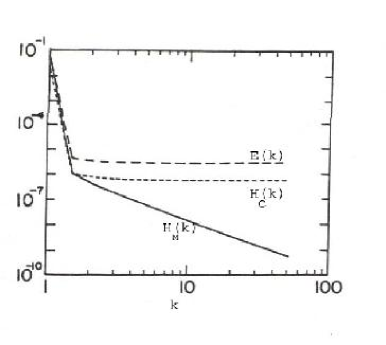
Figure 8: Spectrum of energy, cross helicity, and magnetic helicity of absolute equilibrium state. Adopted from Stribling et al. Stri:Abso .

Clearly total energy and cross helicity appear to cascade to larger wavenumbers, and magnetic helicity is peaking at smaller wavenumbers.

Even though nature of inviscid flow is very different from turbulent flow, Kraichnan and Chen KraiChen suggested that the tendency of the energy cascade in turbulent flow could be anticipated from the absolute equilibrium states. Suppose energy or helicity is injected in some intermediate range, and if the inviscid spectrum peaks at high wavenumber, then one may expect a direct cascade. On the contrary, if the inviscid spectrum peaks at smaller wavenumber, then we expect an inverse cascade. Frisch Fris:HM and Stribling and Matthaeus Stri:Abso have done detailed analysis, and shown that the energy and cross helicity may have forward cascade, and magnetic helicity may have an inverse cascade.

Ting et al. Ting studied the absolute equilibrium states for 2D inviscid MHD. They concluded that energy peaks at larger wavenumbers compared to cross helicity and mean-square vector potential. Hence, energy is expected to have a forward cascade. This is a very interesting property because we can get reasonable information about 3D energy spectra and fluxes by doing 2D numerical simulation, which are much cheaper compared to 3D simulations.

IV.4 Spectrum of Magnetic Helicity and Cross Helicity

As discussed in the previous subsection, absolute equilibrium states of MHD suggest a forward energy cascade for energy and cross helicity, and an inverse cascade for magnetic helicity (3D) or mean-square vector potential (2D). The forward energy cascade has already been discussed in subsection IV.2. Here we will discuss the phenomenologies for the inverse cascade regime.

The arguments are similar to the derivation of Kolmogorov’s spectrum for fluid turbulence (Sec. IV.1). We postulate a constant negative flux of magnetic helicity $\Pi_{H_{M}}$ at low wavenumbers (see Fig. 9).

Figure 9: Cascade direction of energy $\Pi_{E}$ and magnetic helicity $\Pi_{H_{M}}$in MHD turbulence.

Hence, the energy spectrum in this range will have the form

$$E(k)\sim\left|\Pi_{H_{M}}\right|^{\chi}k^{\psi}.$$

Simple dimensional matching yields $\chi=2/3$ and $\psi=-1$. Hence

$$E(k)\sim\left|\Pi_{H_{M}}\right|^{2/3}k^{-1}.$$

We will show later that the inverse cascade of magnetic helicity assists the growth of magnetic energy at large-scales, a process known as “dynamo”.

Using similar analysis for 2D MHD, Biskamp showed that

$$E(k)\sim\left|\Pi_{A2}\right|^{2/3}k^{-1/3},$$

where $\Pi_{A2}$ is the flux of mean-square vector potential. Note however that in 2D fluid turbulence, energy has inverse cascade, but enstrophy ($\Omega=\int|\nabla\times\mathbf{u}|^{2}/2$) has forward cascade (Kraichnan Krai:71 ), and the energy spectrum is

$$E(k) \sim \Pi^{2/3}k^{-5/3}\,\,\,\,\,k\ll k_{f}$$

$$E(k) \sim \Pi_{\Omega}^{2/3}k^{-3}\,\,\,\,\,\,k\gg k_{f},$$

where $k_{f}$ is the forcing wavenumber, and $\Pi_{\Omega}$ is the enstrophy flux.

IV.5 Dynamic Alignment

In a decaying turbulence, energy decreases with time. Researchers found that the evolution of other global quantities also have very interesting properties. Matthaeus et al. Matt:DynaicAlign studied the evolution of normalized cross helicity $2H_{c}/E$ using numerical simulations and observed that it increases with time. In other words, cross helicity decays slower than energy. Matthaeus et al. termed this phenomena as dynamic alignment because higher normalized cross helicity corresponds to higher alignment of velocity and magnetic field. Pouquet et al. Pouq:HcGrowth also observed growth of normalized cross helicity in their simulation. The argument of Matthaeus et al. Matt:DynaicAlign to explain this phenomena is as follows:

In KID’s model of MHD turbulence, the energy fluxes $\Pi^{+}$ and $\Pi^{-}$ are equal (see Eq. [100]). Hence both $E^{+}$ and $E^{-}$ will get depleted at the same rate. If initial condition were such that $E^{+}>E^{-}$, then $E^{+}/E^{-}$ ratio will increase with time. Consequently $\sigma_{c}=(E^{+}-E^{-})/(E^{+}+E^{-})$ will also increase with time.

However, recent development in the field show that Kolmogorov-like phenomenology (Marsch Mars:Kolm , Goldreich and Sridhar Srid1 ; Srid2 , Verma MKV:B0_RG ) models the dynamics of MHD turbulence better than KID’s phenomenology. Keeping this in mind, we generalize the arguments of Matthaeus et al. The rate of change of $E^{+}/E^{-}$is

$$\frac{d}{dt}\frac{E^{+}}{E^{-}}=\frac{1}{\left(E^{-}\right)^{2}}\left[E^{-}\dot{E^{+}}-E^{+}\dot{E^{-}}\right].$$

Clearly, $E^{+}/E^{-}$ will increase with time if

$$\frac{\dot{E^{+}}}{\dot{E^{-}}}>\frac{E^{+}}{E^{-}}\,\,\,or\,\,\,\frac{\epsilon^{+}}{\epsilon^{-}}<\frac{E^{+}}{E^{-}}$$ (110)

using $-\dot{{E^{\pm}}}=\epsilon^{\pm}$. If we assume $E^{+}/E^{-}\sim E^{+}(k)/E^{-}(k)$, then Eq. (103) yields

$$\frac{E^{+}}{E^{-}}\sim\frac{K^{+}}{K^{-}}\left(\frac{\epsilon^{+}}{\epsilon^{-}}\right)^{2}.$$

When $E^{+}/E^{-}$ is not much greater than 1, $K^{+}$and $K^{-}$ are probably very close. Hence,

$$\frac{E^{+}}{E^{-}}\sim\left(\frac{\epsilon^{+}}{\epsilon^{-}}\right)^{2}>\left(\frac{\epsilon^{+}}{\epsilon^{-}}\right).$$

Therefore, according to Eq. (110) $E^{+}/E^{-}$ will increase with time in this limit. For the case $E^{+}/E^{-}\gg 1$, Verma MKV:MHD_Flux showed that

$$\frac{\epsilon^{+}}{\epsilon^{-}}\approx\frac{1}{0.4}.$$

Since $E^{+}/E^{-}\gg 1$, $E^{+}/E^{-}>\epsilon^{+}/\epsilon^{-}$. Hence, growth of normalized cross helicity $\sigma_{c}$ is consistent with Kolmogorov-like model of MHD turbulence.

The above arguments are not applicable when the initial $\sigma_{c}=0$. Numerically simulations show that $\sigma_{c}$ typically could deviate up to 0.1-0.15. Also, cross helicity is quite sensitive to phases of Fourier modes; we will discuss this phenomena in Section IV.7. It would be interesting to study the evolution of cross helicity in the language of symmetry-breaking and its possible generalization to nonequilibrium situations.

IV.6 Selective Decay

We saw in the previous section that the cross helicity $(E^{+}-E^{-})$ decays slower than energy $(E^{+}+E^{-})$. Let us look at it from the decay equation of global quantities:

$$\frac{dE}{dt} = \frac{d}{dt}\int d\tau\frac{1}{2}(u^{2}+b^{2})=-\nu\int d\tau\left|\bigtriangledown\times\mathbf{u}\right|^{2}-\eta\int d\tau j^{2},$$

$$\frac{dH_{c}}{dt} = \frac{d}{dt}\int d\tau\mathbf{u}\cdot\mathbf{B}=-(\nu+\eta)\int d\tau\mathbf{j}\cdot\bigtriangledown\times\mathbf{u}$$

$$\frac{dH_{M}}{dt} = \frac{d}{dt}\int d\tau\frac{1}{2}\left(\mathbf{A}\cdot\mathbf{B}\right)=-\frac{1}{2}\eta\int d\tau\mathbf{j}\cdot\mathbf{B}.$$

where $\mathbf{j}$ represents the current density. Since the dissipation terms of $H_{M}$ has lower power of spatial derivatives as compared to $E$, $H_{M}$ will decay slower than $E$. The decay rate of $H_{c}$ is slower because $H_{C}$ can take both positive and negative values. Hence, $H_{c}$ and $H_{M}$ decay slower than $E$. This phenomena is called selective decay, first proposed by Matthaeus and Montgomery Matt:Selective-decay .

Several researchers argued that turbulence may relax to minimum energy state under the constraint of constant magnetic helicity $H_{M}$. This condition can be written as

$$\delta\left(\int d\tau\frac{1}{2}(u^{2}+b^{2})-\lambda\int d\tau\frac{1}{2}\left(\mathbf{A}\cdot\mathbf{B}\right)\right)=0.$$

Variation with respect to $\mathbf{A}$ yields

$$\bigtriangledown\times\mathbf{B}-\lambda\mathbf{B}=0.$$

Variation with relative to $\mathbf{u}$ yields $\mathbf{u=0}$. The above equation imply that current $\mathbf{j}=\bigtriangledown\times\mathbf{B}$ is parallel to $\mathbf{B}$, therefore force $\mathbf{j\times B}=0$. Hence, the minimum-energy state is a static force-free field. This result finds application in reversed-field-pinch plasma.

Slow decay or growth due to inverse cascade could produce coherent structure. This process is referred to as self-organization process. See Yanase et al. Yana:Coherent for more detailed study of this phenomena.

IV.7 “Phase” Sensitivity of Global Quantities

Let us consider the complex Fourier mode $\mathbf{z}^{\pm}\left(\mathbf{k}\right)=\left|\mathbf{z}^{\pm}\left(\mathbf{k}\right)\right|\exp\left(i\theta^{\pm}\right)$. Clearly there are four independent variables. The $\left|\mathbf{z}^{+}\left(\mathbf{k}\right)\right|$ and $\left|\mathbf{z}^{-}\left(\mathbf{k}\right)\right|$ fix $E^{+}\left(\mathbf{k}\right)$ and $E^{-}\left(\mathbf{k}\right)$ respectively. Since $E^{R}=Re(\mathbf{z}^{+}\left(\mathbf{k}\right)\cdot\mathbf{z}^{-*}\left(\mathbf{k}\right))\propto(E^{u}-E^{b})$, $\theta^{+}-\theta^{-}$ together with $\left|\mathbf{z}^{\pm}\left(\mathbf{k}\right)\right|$ fix $E^{u}/E^{b}$. Hence, three global quantities $(E^{\pm},E^{R})$ or $(E^{u},E^{b},H_{c})$ are fixed by $\left|\mathbf{z}^{\pm}\left(\mathbf{k}\right)\right|$ and $\theta^{+}-\theta^{-}$, leaving the absolute value of $\theta^{+}$ free. Dar et al. Dar:Phase studied the evolution of global quantities by varying the absolute value of initial phase $\theta^{+}$ while keeping $\theta^{+}-\theta^{-}$ fixed. We term this as “phase”.

Dar et al. Dar:Phase performed DNS on $512^{2}$ grid. They performed one set of run (mhd) for random values of $\theta^{+}$ keeping $\theta^{+}-\theta^{-}$ fixed (by choosing appropriate $r_{A})$. In the second run (mhd*) they changed $\theta^{+}$ uniformly for all the modes by an amount $\Delta$, and the third run (mhd**) the phase $\theta^{+}$ were shifted by a random amount. Dar et al. found that total energy and Alfvén ratio do not depend on the shift of $\theta^{+}$, however cross helicity depends quite sensitively on the shift, specially when $\sigma_{c}$ is small. This result is illustrated in Fig. 10.

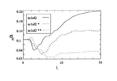
Figure 10: Evolution of normalized cross helicity $\sigma_{c}$ for initial $\sigma_{c}=0.1,$ $r_{A}=0.5$. The curves correspond to three different set of “phases” . Adopted from Dar et al. Dar:Phase .

Dar et al.’s result is very surprising, and its consequences have not been studied in detail. This result raises the question on randomness of initial conditions, ergodicity etc.

In this section we studied some of the basic phenomenological models of MHD turbulence. We will compare their predictions with the numerical results and solar wind observations. These are the topics of discussion of the next two sections.

V Solar Wind: A Testbed for MHD Turbulence

Analytical results are very rare in turbulence research because of complex nature of turbulence. Therefore, experiments and numerical simulations play very important role in turbulence research. In fluid turbulence, engineers have been able to obtain necessary information from experiments (e.g., wind tunnels), and successfully design complex machines like aeroplanes, spacecrafts etc. Unfortunately, terrestrial experiments exhibiting MHD turbulence are typically impossible because of large value of resistivity and viscosity of plasmas. For example, hydrogen plasma at temperature $10^{4}$K has resistivity approximately $10^{5}cm^{2}/s$ (see Table 1). For a typical laboratory setup of size $10cm$ and velocity scale of $10cm/s$, magnetic Reynolds number will be $10^{-3}$, which is far from turbulent regime. On the other hand, astrophysical plasmas have large length and velocity scales, and are typically turbulent. They are a natural testbed for MHD turbulence theories. We have been able to make large set of measurements on nearest astrophysical plasma, the solar wind, using spacecrafts. The data obtained from these measurements have provided many interesting clues in understanding the physics of MHD turbulence. Direct or indirect measurements on planetary and solar atmosphere, galaxies etc. also provide us with useful data, and MHD turbulence is applied to understand these astrophysical objects; due to lack of space, we will not cover these astrophysical objects in our review.

The Sun (or any typical star) spews out plasma, called solar wind. This was first predicted by Parker in 1958, and later observed by spacecrafts. The flow starts at the corona base and extends radially outward beyond the planetary system, and terminates at around 100 AU (1 AU = Earth’s orbital radius$\approx 1.5\times 10^{8}km$). Typical observational data for the solar wind and the corona base is given in Table 4 BiskTurb:book .

Table 4: Typical Observational Data on the Solar Wind

Quantity	Corona Base	1 AU
Ion Density	$10^{9}$$cm^{-3}$	3-20 $cm^{-3}$
Mean Velocity field	300-800 $km/s$	300-800 $km/s$
Velocity fluctuations	?	10-20 $km/s$
Mean magnetic field	$10Gauss$	$(3-20)\times 10^{-5}Gauss$
Magnetic field fluctuations	?	$(1-3)\times 10^{-5}Gauss$
Temperature	$10^{6}$	$10^{4}-10^{6}$

The density of the wind decreases approximately as $r^{-2}$. The mean magnetic field is largely polar in north-south direction, but spirals out in the equatorial plane. Typical Sound speed ($C_{s}\approx\sqrt{{k_{B}T/m_{p}}}$) is of the order of several hundred km/s. The density fluctuation $\delta\rho/\rho\approx(u/C_{s})^{2}\approx 0.01$, hence solar wind can be treated as incompressible fluid.

The solar wind data has been analyzed by many scientists. For details the reader is referred to reviews by Goldstein et al. Gold:RevAnnual and Tu and Marsch TuMars:book . The Alfvén ratio $r_{A}$, which is the ratio of kinetic to magnetic energy, is dependent on heliocentric distance and length-scale. The average value of $r_{A}$ in the inertial range decreases from near 5 at 0.3 AU to near 0.5 at 1AU and beyond MattGold ; Robe:87a ; Robe:87b . The normalized cross helicity $\sigma_{c}$, in general, decreases with increasing heliocentric distance, with asymptotic values near $+1$ (purely outward propagating Alfvén waves) near 0.3 AU, and near 0 by 8 AU or so MattGold ; Robe:87a ; Robe:87b . See Fig. 11 for an illustration.

Now let is focus on energy spectrum and turbulent dissipation rates in the solar wind. Matthaeus and Goldstein MarsTu90 computed the exponent of the total energy and magnetic energy. They found the exponents to be $1.69\pm 0.08$ and $1.73\pm 0.08$ respectively, somewhat closer to 5/3 than 3/2. Similar results were obtained by Marsch and Tu MarsTu90 for $E^{\pm}(k)$ and $E^{u,b}(k)$ at various heliocentric distances. Fig. 11 illustrates the energy spectra $E^{\pm,u,b}(k)$ of a typical solar wind stream. This is surprising because $B_{0}\gg\sqrt{kE^{\pm}(k)}$ for inertial range wavenumbers in the solar wind, and according to KID’s phenomenology, the exponent should be 3/2 (see Section IV.2). The phenomenological model of Matthaeus and Zhou, and Zhou and Matthaeus ZhouMatt ; MattZhou predicts that KID’s phenomenology should hold when $\sqrt{kE^{\pm}(k)}\ll B_{0}$(high $k$), and Kolmogorov-like phenomenology should be to be applicable when $\sqrt{kE^{\pm}(k)}\gg B_{0}$(low $k$). We do not find any such break from 5/3 to 3/2 spectrum in the observed spectrum, thus ruling out phenomenological model of Matthaeus and Zhou, and Zhou and Matthaeus ZhouMatt ; MattZhou .

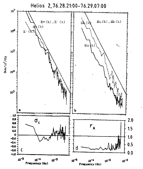
Figure 11: Energy spectra $E^{\pm,u,b}(k)$ of a typical solar wind stream. The normalized cross helicity $\sigma_{c}$ and Alfvén ratio $r_{A}$ are also shown in the figure. Adopted from Tu and Marsch TuMars91

The observational studies of Tu and Marsch TuMars:book show that the spectral index for large cross helicity is also close to $5/3$. This is in contradiction to Grappin et al.’s predictions $\Pi^{+}/\Pi^{-}\approx m^{+}/m^{-}=(3-m^{-})/(3-m^{+})$ Grap82 ; Grap83 . Hence the solar wind observations invalidate the phenomenology of Grappin et al. as well. On the whole, the solar wind data appears to indicate that Kolmogorov-like model (5/3) is applicable in MHD turbulence, even when the mean magnetic field is large as compared to the fluctuations. As we will discuss in later sections, numerical simulations and analytic arguments also support this observation.

As discussed above, the Alfvén ratio ($r_{A}=$$E^{u}/E^{b})$ is high ($\approx 5$) in the inner heliosphere, and it decreases to near 0.5 at 1AU. Similar evolution is seen in numerical simulations as well. In Section VIII.2 we will discuss a plausible argument why Alfvén ratio evolves toward 1 or lower in decaying turbulence.

Temperature of the solar wind decreases slower that adiabatic cooling, implying that solar wind is heated as it evolves. Some of the studied mechanism for heating are turbulence, shocks, neutral ions etc. Tu Tu:Dissipation , Verma et al. MKV:SWheat , Matthaeus et al. Matt:Dissipation , Verma MKV:MHD_Flux , and others have estimated the turbulent dissipation rate in the solar wind from the observational data and modelling. They argued that turbulent heating can contribute significantly to heating of the solar wind.

There are interesting studies on coherent structures, compressibility, density spectrum etc. in the solar wind. Due to lack of space, we will not discuss them here and refer the readers to excellent reviews on solar wind Gold:RevAnnual ; TuMars:book .

VI Numerical Investigation of MHD Turbulence

Like experiments, numerical simulations help us test existing models and theories, and inspire new one. In addition, numerical simulations can be performed for conditions which may be impossible in real experiments, and all the field components can be probed everywhere, and at all times. Recent exponential growth in computing power has fueled major growth in this area of research. Of course, numerical simulations have limitations as well. Even the best computers of today cannot resolve all the scales in a turbulent flow. We will investigate these issues in this section.

There are many numerical methods to simulate turbulence on a computer. Engineers have devised many clever schemes to simulate flows in complex geometries; however, their attention is typically at large scales. Physicists normally focus on intermediate and small scales in a simple geometry because these scales obey universal laws. Since nonlinear equations are generally quite sensitive, one needs to compute both the spatial and temporal derivatives as accurately as possible. It has been shown that spatial derivative could be computed “exactly” using Fourier transforms given enough resolutions Canu:book . Therefore, physicists typically choose spectral method to simulate turbulence. Note however that several researchers (for example, Brandenburg Bran:rev_computation ) have used higher order finite-difference scheme and have obtained comparable results.

VI.1 Numerical Solution of MHD Equations using Pseudo-Spectral Method

In this subsection we will briefly sketch the spectral method for 3D flows. For details refer to Canuto et al. Canu:book . The MHD equations in Fourier space is written as

$$\frac{\partial\mathbf{z^{\pm}}\left(\mathbf{k},t\right)}{\partial t} = \pm i\left(\mathbf{B}_{0}\cdot\mathbf{k}\right)\mathbf{z^{\pm}}\left(\mathbf{k},t\right)-i\mathbf{k}p\left(\mathbf{k},t\right)-FT\left[\mathbf{z^{\mp}}\left(\mathbf{k},t\right)\cdot\nabla\mathbf{\mathbf{z^{\pm}}\left(\mathbf{k},t\right)}\right]$$

$$-\nu_{\pm}k^{2}\mathbf{z^{\pm}}\left(\mathbf{k},t\right)-\nu_{\mp}k^{2}\mathbf{z^{\mp}}\left(\mathbf{k},t\right)+\mathbf{f}^{\pm}(\mathbf{k},t),$$

where $FT$ stands for Fourier transform, and $\mathbf{f}^{\pm}(\mathbf{k},t)$ are forcing functions. The flow is assumed to be incompressible, i. e., $\mathbf{k}\cdot\mathbf{z^{\pm}}\left(\mathbf{k},t\right)=0$. We assume periodic boundary condition with real-space box size as $(2\pi)\times(2\pi)\times(2\pi)$, and Fourier-space box size as $(nx,ny,nz)$. The allowed wavenumbers are ${\textbf{k}}=(k_{x},k_{y},k_{z})$ with $k_{x}=(-n_{x}/2:n_{x}/2),k_{y}=(-n_{y}/2:n_{y}/2),k_{z}=(-n_{z}/2:n_{z}/2)$. The reality condition implies that $\mathbf{z^{\pm}}\left(\mathbf{-k}\right)=\mathbf{z^{\pm*}}\left(\mathbf{k}\right)$, therefore, we need to consider only half of the modes Canu:book . Typically we take $(-n_{x}/2:n_{x}/2,-n_{y}/2:n_{y}/2,0:n_{z}/2)$, hence, we have $N=n_{x}*n_{y}*(n_{z}/2+1)$ coupled ordinary differential equations. The objective is to solve for the field variables at a later time given initial conditions. The following important issues are involved in this method:

1. The MHD equations are converted to nondimensionalized form, and then solved numerically. The parameter $\nu$ is inverse Reynold’s number. Hence, for turbulent flows, $\nu$ is chosen to be quite small (typically $10^{-3}$ or $10^{-4}$). In Section IV.1 we deduced using Kolmogorov’s phenomenology that the number of active modes are

   $$N\sim\nu^{-9/4}.$$

   If we choose a moderate Reynolds number $\nu^{-1}=10^{4}$, $N$ will be $10^{9}$, which is a very large number even for the most powerful supercomputers. To overcome this difficulty, researchers apply some tricks; the most popular among them are introduction of hyperviscosity and hyperresistivity, and large-eddy simulations. Hyperviscous (hyperresistive) terms are of the form $(\nu_{j},\eta_{j})k^{2j}\mathbf{\mathbf{z^{\pm}}\left(\mathbf{k}\right)}$ with $j\geq 2$; these terms become active only at large wavenumbers, and are expected not to affect the inertial range physics, which is of interest to us. Because of this property, the usage of hyperviscosity and hyperresistivity has become very popular in turbulence simulations. Large-eddy simulations will be discussed in Section XII of this paper. Just to note, one of the highest resolution fluid turbulence simulation is by Gotoh Goto:DNS on a $4096^{3}$ grid; this simulation was done on Fujitsu VPP5000/56 with 32 processors with 8 Gigabytes of RAM on each processor, and it took 500 hours of computer time.

2. The computation of the nonlinear terms is the most expensive part of turbulence simulation. A naive calculation involving convolution will take $O(N^{2})$ floating point operations. It is instead efficiently computed using Fast Fourier Transform (FFT) as follows:
   (a) Compute $\mathbf{\mathbf{z^{\pm}}\left(x\right)}$ from $\mathbf{\mathbf{z^{\pm}}\left(\mathbf{k}\right)}$ using Inverse FFT.
   (b) Compute $z_{i}^{\mp}({\textbf{x}})z_{j}^{\pm}({\textbf{x}})$ in real space by multiplying the fields at each space points.
   (c) Compute $FFT[z_{i}^{\mp}({\textbf{x}})z_{j}^{\pm}({\textbf{x}})]$ using FFT.
   (d) Compute $ik_{j}FFT[z_{i}^{\mp}({\textbf{x}})z_{j}^{\pm}({\textbf{x}})]$ by multiplying by $k_{j}$ and summing over all $j$. This vector is $-FFT\left[\mathbf{z^{\mp}}\left(\mathbf{k},t\right)\cdot\nabla\mathbf{\mathbf{z^{\pm}}\left(\mathbf{k},t\right)}\right]$.
   Since FFT takes $O(N\log N)$, the above method is quite efficient. The multiplication is done in real space, therefore this method is called pseudo-spectral method instead of just spectral method.

3. Products $z_{i}^{\mp}({\textbf{x}})z_{j}^{\pm}({\textbf{x}})$ produce modes with wavenumbers larger than $k_{max}$. On FFT, these modes get aliased with $k<k_{max}$ and will provide incorrect value for the convolution. To overcome this difficulty, last 1/3 modes of fields $z_{i}^{\pm}(\mathbf{k})$ are set to zero (zero padding), and then FFTs are performed. This scheme is called $2/3$ rule. For details refer to Canuto et al. Canu:book .

4. Pressure is computed by taking the dot product of MHD equation with $\mathbf{k}$. Using incompressibility condition one obtains

   $$p\left(\mathbf{k},t\right)=\frac{i\mathbf{k}}{k^{2}}\cdot FT\left[\mathbf{z^{\mp}}\left(\mathbf{k},t\right)\cdot\nabla\mathbf{\mathbf{z^{\pm}}\left(\mathbf{k},t\right)}\right].$$

   To compute $p({\textbf{k}})$ we use already computed nonlinear term.

5. Once the right-hand side of the MHD equation could be computed, we could time advance the equation using one of the standard techniques. The viscous terms are advanced using an implicit method called Crank-Nicholson’s scheme. However, the nonlinear terms are advanced using Adam-Bashforth or Runge-Kutta scheme. One uses either second or third order scheme. Choice of $dt$ is determined by CFL criteria $(dt<(\bigtriangleup x)/U_{rms})$. By repeated application of time-advancing, we can reach the desired final time.

6. The MHD turbulence equations can be solved either using $\mathbf{z^{\pm}}$ or $\mathbf{\left(\mathbf{u},b\right)}$. The usage of $\mathbf{z^{\pm}}$ turns out to be more efficient because they involve less number of FFT operations.

7. When forcing $\mathbf{f}^{\pm}=0$, the total energy gets dissipated due to viscosity and resistivity. This is called decaying simulation. On the contrary, forced simulation have nonzero forcing $(\mathbf{f}\neq 0)$, which feed energy into the system, and the system typically reaches a steady-state in several eddy turnover time. Forcing in astrophysical and terrestrial systems are typically at large-scale eddies (shocks, explosions etc.). Therefore, in forced MHD equations $\mathbf{f}^{u}$ is typically applied at small wavenumbers, which could feed both kinetic energy and kinetic helicity. For details refer to Brandenburg Bran:Alpha .

Spectral method has several disadvantages as well. This method can not be easily applied to nonperiodic flows. That is the reason why engineers hardly use spectral method. Note however that even in aperiodic flows with complex boundaries, the flows at small length-scale can be quite homogeneous, and can be simulated using spectral method. Spectral simulations are very popular among physicists who try to probe universal features of small-scale turbulent flows. Since the MHD equations are solved directly (without any modeling), this method is called Direct Numerical Simulation (DNS).

Many researchers have done spectral simulation of MHD turbulence. In this section we will mention some of the main results concerning energy spectra and cascade rates. Numerical results on dynamo and intermittency will be discussed later in this paper. Some numerical results on the evolution of global quantities (e. g., dynamic alignment by Matthaeus et al. Matt:DynaicAlign ) were discussed were discussed in Section IV, and they will not be repeated here.

VI.2 Numerical Results on Energy Spectra (3/2 or 5/3)

In Sec. IV we discussed various MHD turbulence phenomenologies, which predict the exponents to be 3/2, or 5/3, or mix of both. Grappin et al. Grap83 predicted the exponents to be cross helicity dependent; for small $\sigma_{c}$, $m^{+}\approx m^{-}\approx 3/2$, but for large $\sigma_{c}$, $m^{+}\rightarrow 3$, and $m^{-}\rightarrow 0$. Many researchers tried to test these predictions numerically.

One-dimensional energy spectrum $E(k)$ is computed by summing over all the modes in the shell $(k-1/2:k+1/2)$, i.e.,

$$E^{X}(k)=\frac{1}{2}\sum_{k-1/2<|\mathbf{s}|<k+1/2}\left|\hat{\mathbf{X}}(\mathbf{s})\right|^{2},$$

where $\mathbf{X}=\mathbf{u},\mathbf{b},\mathbf{z}^{\pm}$. The Energy spectrum is computed for both decaying or forced simulations. In the final state (after 2-10 eddy turnover time), Alfvén ratio is typically found to be close to 1/2. Most of the MHD turbulence simulations have been done for zero cross helicity; for these cases, normalized cross helicity typically fluctuates in the range of $-0.1$ to 0.1.

Most of the high resolution simulations till early 1990s were done in 2D due to lack of computing resources. Biskamp and Welter BiskWelt performed numerical studies of 2D MHD turbulence on grid up to $1024^{2}$ under small cross helicity limit. They reported the spectral index to be close to $3/2$ in agreement with the models of Kraichnan, Iroshnikov, and Dobrowolny et al. (KID), with a caveat that the exponents may be close to 5/3 in transition states, in which turbulence is concentrated in regions of weak magnetic field. In summary, the numerical simulations till early 1990s supported 3/2 spectral index. Note that according to absolute equilibrium theory, 2D and 3D are expected to have the same energy spectra. So we can test the turbulence models in 2D as well.

Since 5/3 and 3/2 are very close, there is a practical difficulty in resolving the spectral index. They can be resolved with certainty only in a high-resolution simulations. Verma MKV:Thesis , and Verma et al. MKV:MHD_Simulation approached this problem indirectly. They tested the energy cascade rates $\Pi^{\pm}$ for nonzero cross helicity in $512^{2}$ DNS. Recall that KID’s model (3/2) predicts $\Pi^{+}=\Pi^{-}$(Eq. [100]) independent of $E^{+}/E^{-}$ ratio, while Kolmogorov-like theories (5/3) predict (Eq. [103])

$$\frac{E^{-}(k)}{E^{+}(k)}=\frac{K^{-}}{K^{+}}\left(\frac{\Pi^{-}}{\Pi^{+}}\right)^{2}.$$

Verma MKV:Thesis and Verma et al. MKV:MHD_Simulation computed both energy spectra and cascade rates; their plots of the energy spectra and fluxes are reproduced in Fig. 12.

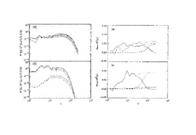
Figure 12: $E^{\pm}(k)k^{a}$ vs. $k$ (left panel) and $\Pi^{\pm}(k)$ vs. $k$ (right panel) for 2D runs with (a) $B_{0}=0$ and initial $\sigma_{c}=0.0$, and (b) $B_{0}=1.0$ and initial $\sigma_{c}=0.9$. In the left panel the solid $(E^{+})$ and dashed line $(E^{-})$ correspond to $a=5/3$, and chained $(E^{+})$ and dotted $(E^{-})$ correspond to $a=3/2$. In the right panel solid and chained lines represent $\Pi^{\pm}$ respectively, while the dashed and dotted lines represent dissipation rate and the energy loss in the sphere of radius $k$. The numerical results favour Kolmogorov’s phenomenology over KID’s phenomenology. Adopted from Verma et al. MKV:MHD_Simulation .

Regarding spectral indices, no particular claim could be made because the numerically computed indices were within the error bars of both 3/2 and 5/3. However, the study of energy fluxes showed that underlying turbulent dynamics is closer to Kolmogorov-like. The energy flux of majority species (larger of $E^{+}$and $E^{-}$, here taken to be $E^{+}$) was always greater that that of minority species, even in situations where $z_{rms}^{\pm}\ll B_{0}$. When we look at the values of cascade rates more closely (see Table 1 of Verma et al. MKV:MHD_Simulation ), we find that ,

$$\frac{E^{-}(k)}{E^{+}(k)}\approx\left(\frac{\Pi^{-}}{\Pi^{+}}\right)^{2}$$ (111)

for initial $\sigma_{c}=0.25$. However, for initial $\sigma_{c}=0.9$, they were off by a factor of 10. The Eq. (111) assumes $K^{+}=K^{-}$, which is not a valid assumption for large $\sigma_{c}$. Verma MKV:MHD_Flux has shown that $K^{\pm}$ depend on $\sigma_{c}$, and the factor of $K^{-}/K^{+}$ is of the order of 4. With this input, the numerical results come closer to the analytical results, but the agreement is still poor. This indicates that physics at large cross helicity (Alfvénic turbulence) is still unresolved.

The above numerical results imply that the relevant time scale for MHD turbulence is nonlinear time-scale $(kz_{k}^{\pm})^{-1}$, not the Alfvén time-scale $(kB_{0})^{-1}$. Verma’s MKV:Thesis and Verma et al.’s MKV:MHD_Simulation provided one of the first numerical evidence that Kolmogorov’s scaling is preferred over KID’s 3/2 scaling in MHD turbulence.

High resolution three-dimensional simulations soon became possible due to availability of powerful computers. Müller and Biskamp Bisk:Kolm1 , and Biskamp and Müller Bisk:Kolm2 performed $512^{3}$ DNS with both normal and hyperdiffusive terms. They showed that the energy spectrum follows a $k^{-5/3}$ law, steeper than $k^{-3/2}$ as previously thought (see Fig. 13).

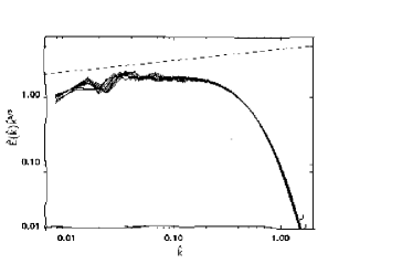
Figure 13: Plot of normalized energy spectrum compensated by $k^{5/3}$for a 3D MHD simulation on $512^{3}$grid. Flatness of the plot indicates that Kolmogorov’s 5/3 index fits better than 3/2 (dashed line). Adopted from Biskamp and Müller Bisk:Kolm2 .

The runs with hyperdiffusivity had a bump at large wavenumbers. The Kolmogorov’s constant was found to be 2.3. The range of 5/3 powerlaw is close to 1 decade. Numerical results of Cho Cho:Simulation , Cho et al. ChoLaz:Viscosity-damped , and others are consistent with Kolmogorov’s scaling.

Biskamp and Müller also computed the intermittency exponents and showed that they are consistent with Kolmogorov scaling and sheet-like dissipative structure. We will discuss these issues later in this paper.

Biskamp and Schwarz Bisk:2D performed DNS on two-dimensional MHD turbulence on grids of $2048^{2}$ to $8192^{2}$. They claimed that the energy spectrum agrees with KID’s law (3/2), contrary to 3D case. They have also computed the structure functions, and reported a strong anomalous bottleneck effect. Note that Biskamp and Schwarz’s results contradicts Verma et al.’s MKV:MHD_Simulation results, where the energy fluxes follow Kolmogorov’s predictions. This issue needs a closer look. It is possible that the dynamics is Kolmogorov-like, but they are strongly modified by intermittency effects. Refer to Verma et al. MKV:Bisk_Comment , Biskamp Bisk:MKV_Comment , and Section XI for further details.

VI.3 Numerical Results on Anisotropic Energy Spectra

Shebalin et al. Sheb performed DNS in 2D and studied the anisotropy resulting from the application of a mean magnetic field. They quantified anisotropy using the angle $\theta_{Q}$ defined by

$$\tan^{2}\theta_{Q}=\frac{\sum k_{\perp}^{2}\left|Q\left(\mathbf{k},t\right)\right|^{2}}{\sum k_{||}^{2}\left|Q\left(\mathbf{k},t\right)\right|^{2}},$$

where $Q$ represents any one of the vector fields like $\mathbf{u},\mathbf{b},\nabla\times\mathbf{u}$ etc. They found turbulence to be anisotropic. Later Oughton et al. Ough carried out the anisotropic studies in 3D. They found that with the increase of $B_{0}$, anisotropy increases up to $B_{0}\sim 3,$ then it saturated. They also found that anisotropy increases with increasing mechanical and magnetic Reynolds numbers, and also with increasing wavenumbers. $B_{0}$ also tended to suppress energy cascade. Matthaeus et al. Matt:AnisotropyPRL numerically show that the anisotropy scales linearly with the ratio of fluctuating to total magnetic field strength.

Cho et al. ChoVish:anis ; ChoVish:localB performed 3D DNS and studied anisotropic spectrum. They found that anisotropy of eddies depended on their size: along “local” magnetic field lines, the smaller eddies are more elongated than the larger ones. See Fig. 14 for an illustration of numerically computed velocity correlation function.

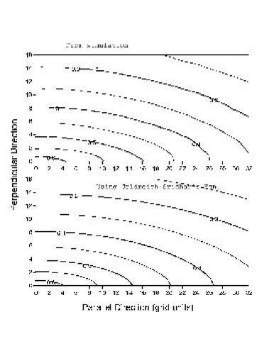
Figure 14: Cho et al. ChoVish:localB compared the velocity correlation function from simulation (top panel) with the predictions of Goldreich and Sridhar’s theory (bottom panel). The results are in very good agreement. Adopted from Cho et al. ChoVish:localB .

The numerical value matched quite closely with the predictions of Goldreich and Sridhar Srid2 . Their result was also consistent with the scaling law $k_{||}\sim k_{\perp}^{2/3}$ proposed by Goldreich and Sridhar Srid2 . Here $k_{||}$ and $k_{\perp}$ are the wavenumbers measured relative to the local magnetic field direction. The “local” magnetic field is in the same spirit as the “effective” mean magnetic field of Verma MKV:B0_RG .

Maron and Goldreich Maro:Simulation performed a detailed DNS of MHD turbulence. Their grid size ranged from $(64^{2}\times 256)$ to $(256^{2}\times 512)$. They numerical results are in general agreement with the Goldreich and Sridhar prediction $k_{||}\sim k_{\perp}^{2/3}$. However, their 1D spectral index was closer to 3/2 than 5/3, contrary to Cho et al. ’s ChoVish:anis ; ChoVish:localB numerical results that $E(k_{\perp})\propto k_{\perp}^{-5/3}$.

After a review of energy spectra in MHD turbulence, we now turn to studies on energy fluxes in MHD turbulence.

VI.4 Numerical Results on Energy Fluxes

Computation of energy fluxes using DNS has done by Verma et al. MKV:MHD_Simulation , Dar et al. Dar:flux , and Ishizawa and Hattori Ishi:EDQNM ; Ishi:flux (using wavelet basis). Verma et al. numerically computed $\Pi^{\pm}$, while Dar et al., and Ishizawa and Hattori computed various fluxes $\Pi_{Y>}^{X<}$ ($X,Y=u,b)$ in 2D MHD turbulence.

Dar et al. performed numerical DNS on a $512^{2}$ grid with random kinetic forcing over a wavenumber annulus $4\leq k\leq 5$. Theoretically, the magnetic energy in two-dimensional MHD decays in the long run even with steady kinetic energy forcing Zeld:book . However, we find that the magnetic energy remains steady for sufficiently long time before it starts to decay. For $128^{2}$ simulation, the decay of magnetic energy starts only after $t=25-30$ time units, and for $512^{2}$, the decay starts much later. We compute the energy fluxes in this quasi steady-state. In the quasi steady-state, the Alfvén ratio fluctuates between 0.4 and 0.56, and the normalized Cross helicity $\sigma_{c}$ approximately equal to 0.1. They found however that a variation of $\sigma_{c}$ does not change the behaviour of flux appreciably.

We illustrate the flux computation using an example. The flux $\Pi_{b>}^{u<}(k_{0})$, which is energy flux from inside of $u$-sphere of radius $k_{0}$, to outside of $b$-sphere of radius $k_{0}$, is

$$\Pi_{b>}^{u<}(k_{0})=\sum_{\mathbf{\left|k^{\prime}\right|<k_{0}}}\sum_{\left|\mathbf{p}\right|<k_{0}}\Im\left(\left[\mathbf{k}^{\prime}\cdot\mathbf{b}(\mathbf{q})\right]\left[\mathbf{b}(\mathbf{k^{\prime}})\cdot\mathbf{u}(\mathbf{p})\right]\right).$$ (112)

Now we define two “truncated” variables ${\textbf{u}}^{<}$ and ${\textbf{b}}^{>}$ as

$${\textbf{u}}^{<}({\textbf{k}})=\left\{\begin{array}[]{ll}{\textbf{u}}({\textbf{k}})&\mbox{if $|{\textbf{k}}|<k_{0}$}\\ 0&\mbox{if $|{\textbf{k}}|>k_{0}$}\end{array}\right.$$ (113)

and

$${\textbf{b}}^{>}({\textbf{p}})=\left\{\begin{array}[]{ll}0&\mbox{if $|{\textbf{p}}|<K$}\\ {\textbf{b}}({\textbf{p}})&\mbox{if $|{\textbf{p}}|>K$}\end{array}\right.$$ (114)

Eq. (112) written in terms of ${\textbf{u}}^{<}$ and ${\textbf{b}}^{>}$ reads as

$$\Pi_{b>}^{u<}(K)=\Im\left[\sum_{\textbf{k}}k_{j}b_{i}^{>}({\textbf{k}})\sum_{\textbf{p}}b_{j}({\textbf{k-p}})u_{i}^{<}({\textbf{p}})\right]$$ (115)

The p summation in the above equation is a convolution, which is computed using FFT. After FFT, $\mathbf{k}$ sum is performed. We compute energy flux this way. Ishizawa and Hattori Ishi:EDQNM ; Ishi:flux used Meyor wavelets as basis vectors and have computed the energy fluxes. Their approach is very similar to that of Dar et al.

The energy fluxes as a function of wavenumber spheres are plotted in Fig. 15.

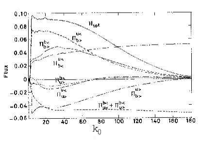
Figure 15: The plots of various energy fluxes in 2D-MHD versus wavenumber for a $512^{2}$ simulation. Adopted from Dar et al. Dar:flux .

The inertial range $20<k<50$ can be deduced from the approximate constancy of the energy fluxes. In Fig. 16 we schematically illustrate the numerical values of fluxes for $k=20$, a wavenumber within the inertial range.

Figure 16: A schematic illustration of the numerically evaluated values of the fluxes averaged over 15 time units. The values shown here are for $k=20,$ a wavenumber within the inertial range. Taken from Dar et al. Dar:flux

The main conclusions of Dar et al.’s calculation are as follows:

1. The sources for the large-scale magnetic field are large-scale velocity field ($\Pi_{b<}^{u<}$) and the small-scale velocity field ($\Pi_{u>}^{b<}$). The former transfer is of a greater magnitude than the latter, hence the magnetic field enhancement is primarily caused by a transfer from the u-sphere to the b-sphere. Indeed the first few b-modes get most of this energy.

2. Energy from the large-scale velocity field gets transferred to the small-scale magnetic field ($\Pi_{b>}^{u<}$). The small-scale magnetic field transfers energy to the small-scale velocity field ($\Pi_{u>}^{b>}$).

3. Small-scale velocity field transfers energy to large-scale velocity as well as magnetic field. Hence, there is an inverse cascade of kinetic energy. This result is consistent with the EDQNM closure calculations Pouq:EDQNM2D ; Ishi:EDQNM .

4. There is a forward cascade of magnetic energy toward the small scales. EDQNM closure calculations also yield a magnetic energy transfer to the small-scales Ishi:EDQNM .

Ishizawa and Hattori Ishi:EDQNM ; Ishi:flux obtained very similar results in their DNS using wavelet basis.

We have performed a preliminary 3D simulation on $512^{3}$ grid size and calculated the energy fluxes Oliv:Simulation . Ours was a decaying simulation in which Alfvén ratio saturated near 0.4. The energy fluxes at $k=11$, one of the inertial range wavenumbers, is shown in Fig. 17.

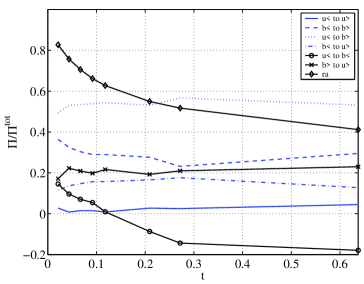
Figure 17: Values of inertial-range energy fluxes at different time in a $512^{3}$ decaying 3D-MHD turbulence simulation. Note the change in sign for some of the fluxes near $r_{A}=0.6$.

All the outgoing fluxes are positive, but $\Pi_{b<}^{u<}$ is negative for $r_{A}<0.6$. These are in qualitative agreement with Verma’s analytic results MKV:MHD_Flux ; Ayye:MHD , which will be discussed in Section VIII.

Haugen et al. Bran:Flux have computed the dissipation rates of kinetic and magnetic energies. They find that for $E^{b}/E^{u}\approx 0.5$, $\epsilon^{u}/\Pi=(\Pi_{u>}^{u<}+\Pi_{u>}^{b<})/\Pi\approx 0.3$, and $\epsilon^{b}/\Pi=(\Pi_{b>}^{u<}+\Pi_{b>}^{b<})/\Pi\approx 0.7$ (see Figures 11 and 12 of Haugen et al. Bran:Flux ). Note however that Haugen et al. ’s schematics of energy fluxes are missing $\Pi_{u>}^{b<}$ and $\Pi_{b>}^{u<}$. We will compare Haugen et al.’s numerical values with theoretical predictions in Section VIII.1.1.

There are major differences between the energy fluxes in 2D and 3D MHD turbulence. Primarily, for $r_{A}<0.6$, $\Pi_{b<}^{u<}<0$ in 3D MHD but is positive in 2D MHD. Also, $\Pi_{u>}^{u<}$ and $\Pi_{u>}^{b<}$ are positive in 3D, but are negative in 2D MHD. In Section VIII we will compare 3D numerical results with their analytical counterparts. Unfortunately, we do not have analytical results for 2D MHD turbulence.

The energy fluxes give us information about the overall energy transfer from inside/outside $u/b$-sphere to inside/outside $u/b$-sphere. To obtain a more detailed account of the energy transfer, Dar et al. Dar:flux also studied energy exchange between the wavenumber shells; Ishizawa and Hattori Ishi:EDQNM ; Ishi:flux performed the same studies using wavelet basis.

VI.5 Shell-to-Shell energy Transfer-rates in MHD Turbulence

Dar et al. Dar:flux partitioned the k-space into shells with boundaries at wavenumbers $k_{n}(n=1,2,3,...)=1,16,19.02,22.62,...,2^{(n+14)/4}$, and computed the shell-to-shell energy transfer rates $T_{nm}^{YX}$ defined by Eq. (84). The results are shown in Fig. 18.

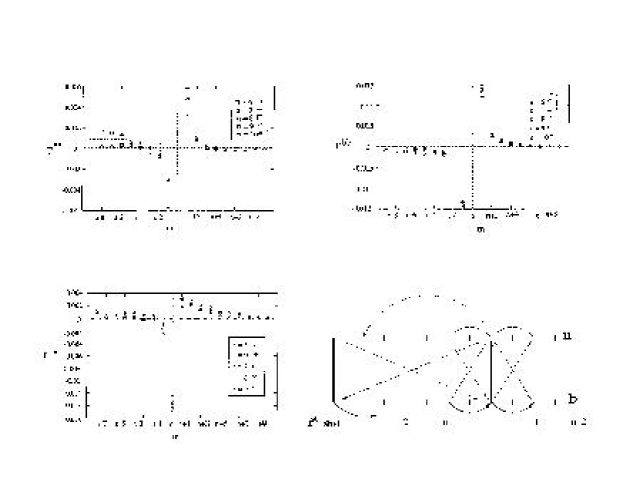
Figure 18: Shell-to-shell energy transfer $T_{nm}^{uu},T_{nm}^{bb},T_{nm}^{bu}$ (in order) for Dar et al.’s $512^{2}$ run. They are schematically illustrated in the last diagram. Adopted from Dar et al. Dar:flux .

The main conclusions of Dar et al. are as follows:

1. The energy fluxes $T_{nm}^{YX}$ are virtually independent of the individual values of $m$ and $n$, but only dependent on their differences. Hence, the transfer rates in the inertial range are self-similar.

2. $T_{nm}^{bb}$ is positive for $n>m$, and negative for $n<m$, and maximum for $n=m+1.$ Hence magnetic to magnetic energy transfer is forward and local.

3. The most dominant $T_{nm}^{uu}$ is from $(m-1)$-th shell to $m$-th shell and $m$-th shell to $(n=m+1)$-th shell, thus $u$-$u$ energy transfer to the nearest shell is forward. However, $T_{nm}^{uu}$ is negative for $n>m+3$, which may contribute to the inverse cascade of kinetic energy. This result is consistent with analytic results on 2D shell-to-shell energy transfers in fluid turbulence (see Appendix D). There are significant energy transfers from inertial wavenumbers to small wavenumbers (nonlocal), which will also contribute to the inverse cascade of energy.

4. $T_{nm}^{bu}$ is positive for all $n$, except for $n=m-1$ and $m$, implying that $n$-th $u$ shell loses energy to all but $n$th and $(n-1)$th $b$-shell. However, energy gained from these two shells is larger than the total loss. Consequently there is a net gain of energy by $u$-shells in the inertial range.

5. $T_{1m}^{bu}$ is positive implying that the first $b$-shell gains energy from the inertial range $u$-shells through a nonlocal transfer.

6. $T_{n1}^{bu}$ is positive implying that the first $u$-shell loses energy to the inertial range $b-$shells through a nonlocal transfer.

All the above results are schematically illustrated in Fig. 18(d).

The above results on shell-to-shell energy transfers provide us with important insights into the dynamics of MHD turbulence. Unfortunately, we do not have enough results on shell-to-shell energy transfer in 3D.

In this section we described the methodology of spectral method and some important results on energy spectra, fluxes, and shell-to-shell transfers. In Section XII we will also present large-eddy simulation (LES), which enables us to perform turbulence simulations on smaller grids. In the next three sections we will describe the field-theoretic calculation of renormalized viscosity and resistivity, energy fluxes, and shell-to-shell energy transfer rates.

VII Renormalization Group Analysis of MHD Turbulence

In Section IV we discussed various existing MHD turbulence models. Till early 1990s, KID’s model (3/2 spectral index) used be the accepted model of MHD turbulence. However, solar wind observations and numerical results in the last decade are in better agreement with the predictions of Kolmogorov-like models (5/3 spectral index). In this and the next two sections we will present computation of energy spectrum and energy cascade rates starting from the MHD equations using field-theoretic techniques. In this section we will present some of the important renormalization group calculations applied to MHD turbulence. Most recent RG calculations favour 5/3 spectral index for energy spectrum.

Field theory is well developed, and has been applied to many areas of physics, e.g., Quantum Electrodynamics, Condensed Matter Physics etc. In this theory, the equations are expanded perturbatively in terms of nonlinear term, which are considered small. In fluid turbulence the nonlinear term is not small; the ratio of nonlinear to linear (viscous) term is Reynolds numbers, which is large in turbulence regime. However in MHD turbulence, when $B_{0}\gg z^{\pm}$, the nonlinear term is small compared to the linear (Alfvén propagation term $\mathbf{B}_{0}\cdot\nabla\mathbf{z}^{\pm}$) term. This is the weak turbulence limit, and the perturbative expansion makes sense here. On the other hand when $z^{\pm}\gg B_{0}$ (the strong turbulence limit), the nonlinear term is not small, and the perturbative expansion is questionable. This problem appears in many areas of physics including Quantum Chromodynamics (QCD), Strongly Correlated Systems, Quantum Gravity etc., and is largely unsolved. Several interesting methods, Direct Interaction Approximation, Renormalization Groups (RG), Eddy-damped quasi-normal Markovian approximations, have been attempted in turbulence. We discuss some of them below.

A simple-minded calculation of Green’s function shows divergence at small wavenumbers (infrared divergence). One way to solve problem is by introducing an infrared cutoff for the integral. The reader is referred to Leslie Lesl:book for details. RG technique, to be described below, is a systematic procedure to cure this problem.

VII.1 Renormalization Groups in Turbulence

Renormalization Group Theory (RG) is a technique which is applied to complex problems involving many length scales. Many researchers have applied RG to fluid and MHD turbulence. Over the years, several different RG applications for turbulence has been discovered. Broadly speaking, they fall in three different categories:

Yakhot-Orszag (YO) Perturbative approach

Yakhot and Orszag’s YakhOrsz work, motivated by Forster et al. FNS and Fournier and Frisch FourFrisRG , is the first comprehensive application of RG to turbulence. It is based on Wilson’s shell-elimination procedure. Also refer to Smith and Woodruff Smit for details. Here the renormalized parameter is function of forcing noise spectrum $D(k)=D_{0}k^{-y}$. It is shown that the local Reynolds number $\bar{\lambda}$ is

$$\bar{\lambda}=\frac{\lambda_{0}^{2}D_{0}}{\nu^{3}(\Lambda)\Lambda^{\epsilon}},$$

where $\lambda_{0}$ is the expansion parameter, $\Lambda$ is the cutoff wavenumber, and $\epsilon=4+y-d$ YakhOrsz . It is found that $\nu(\Lambda)$ increases as $\Lambda$ decreases, therefore, $\bar{\lambda}$ remains small (may not be less that one though) compared to $Re$ as the wavenumber shells are eliminated. Hence, the “effective” expansion parameter is small even when the Reynolds number may be large.

The RG analysis of Yakhot and Orszag YakhOrsz yielded Kolmogorov’s constant $K_{Ko}=1.617$, turbulent Prandtl number for high-Reynolds-number heat transfer $P_{t}=0.7179$, Batchelor constant $Ba=1.161$ etc. These numbers are quite close to the experimental results. Hence, Yakhot and Orszag’s method appears to be highly successful. However there are several criticisms to the YO scheme. Kolmogorov’s spectrum results in the YO scheme for $\epsilon=4$, far away from $\epsilon=0$, hence epsilon-expansion is questionable. YO proposed that higher order nonlinearities are “irrelevant” in the RG sense for $\epsilon=0$, and are marginal when $\epsilon=4$. Eyink Eyin:RG objected to this claim and demonstrated that the higher order nonlinearities are marginal regardless of $\epsilon$. Kraichnan Krai:YO compared YO’s procedure with Kraichnan’s Direct Interaction Approximation Krai:59 and raised certain objections regarding distant-interaction in YO scheme. For details refer to Zhou et al. ZhouMcCo:RGrev and Smith and Woodruff Smit .

There are several RG calculations applied to MHD turbulence based on YO procedure. These calculations will be described in Section VII.5.

Self-consistent approach of McComb and Zhou

This is one of the nonperturbative method, which is often used in Quantum Field theory. In this method, a self-consistent equation of the full propagator is written in terms of itself and the proper vertex part. The equation may contain many (possibly infinite) terms, but it is truncated at some order. Then the equation is solved iteratively. McComb McCo:book , Zhou and coworkers ZhouVaha88 have applied this scheme to fluid turbulence, and have calculated renormalized viscosity and Kolmogorov’s constant successfully. Direct Interaction Approximation of Kraichnan is quite similar to self-consistent theory (Smith and Woodruff Smit ).

The difficulty with this method is that it is not rigorous. In McComb and Zhou’s procedures, the vertex correction is not taken into account. Verma MKV:B0_RG ; MKV:MHD_PRE ; MKV:MHD_RG has applied the self-consistent theory to MHD turbulence.

Callan-Symanzik Equation for Turbulence

DeDominicis and Martin DeDo and Teodorovich Teod obtained the RG equation using functional integral. Teodorovich obtained $K_{Ko}=2.447$, which is in worse agreement with the experimental data, though it is not too far away.

It has been shown that Wilson’s shell renormalization and RG through Callan-Symanzik equation are equivalent procedure. However, careful comparison of RG schemes in turbulence is not completely worked out.

The renormalization of viscosity, resistivity, and “mean magnetic field” will be discussed below. The self-consistent approach will be discussed at somewhat greater length because it is one of the most recent and exhaustive work. After renormalization, in Section VIII we will discuss the computation of energy fluxes in MHD turbulence. These calculations are done using self-consistent field theory, a scheme very similar to DIA. At the end we will describe Eddy-damped quasi-normal Markovian approximation, which is very similar to the energy flux calculation.

VII.2 Physical Meaning of Renormalization in Turbulence

The field theorists have been using renormalization techniques since 1940s. However, the physical meaning of renormalization became clear after path-breaking work of Wilson WilsKogu . Here renormalization is a variation of parameters as we go from one length scale to the next. Following Wilson, renormalized viscosity and resistivity can also be interpreted as scale-dependent parameters. We coarse-grain the physical space and look for an effective theory at a larger scale. In this method, we sum up all the interactions at smaller scales, and as a outcome we obtain terms that can be treated as a correction to viscosity and resistivity. The corrected viscosity and resistivity are called “effective” or renormalized dissipative parameters. This procedure of coarse graining is also called shell elimination in wavenumber space. We carry on with this averaging process till we reach inertial range. In the inertial range the “effective” or renormalized parameters follow a universal powerlaw, e. g., renormalized viscosity $\nu(l)\propto l^{4/3}$. This is the renormalization procedure in turbulence. Note that the renormalized parameters are independent of microscopic viscosity or resistivity.

In viscosity and resistivity renormalization the large wavenumber shells are eliminated, and the interaction involving these shells are summed. Hence, we move from larger wavenumbers to smaller wavenumbers. However, it is also possible to go from smaller wavenumbers to larger wavenumber by summing the smaller wavenumber shells. This process is not coarse-graining, but it is a perfectly valid RG procedure, and is useful when the small wavenumber modes (large length scales) are linear. This scheme is followed in Quantum Electrodynamics (QED), where the electromagnetic field is negligible at a large distance (small wavenumbers) from a charge particle, while the field becomes nonzero at short distances (large wavenumber). In QED, the charge of a particle gets renormalized when we come closer to the charge particle, i. e., from smaller wavenumbers to larger wavenumbers. In MHD too, the large-scale Alfvén modes are linear, hence we can apply RG procedure from smaller wavenumbers to larger wavenumbers. Verma MKV:B0_RG has precisely done this to compute the “effective or renormalized mean magnetic field” in MHD turbulence. See Fig. 19 for an illustration of wavenumber shells to be averaged.

Figure 19: The wavenumber shells to be averaged during renormalization procedure. (a) In “mean magnetic field” renormalization, averaging starts from small wavenumber, first shell being $(k_{0},k_{1})$. (b) In viscosity and resistivity, averaging starts from large wavenumbers.

VII.3 “Mean Magnetic Field” Renormalization in MHD Turbulence

In this subsection we describe the self-consistent RG procedure of Verma MKV:B0_RG , which is similar to that used by McComb McCo , McComb and Shanmugsundaram McCoShan , McComb and Watt McCoWatt , and Zhou et al. ZhouVaha88 for fluid turbulence. However, one major difference between the two is that Verma MKV:B0_RG integrates the small wavenumber modes instead of integrating the large wavenumber modes, as done by earlier authors. At small wavenumbers the MHD equations are linear in $B_{0}$, the mean magnetic field. Verma applied RG procedure to compute the renormalized mean magnetic field.

The basic idea of the calculation is that the effective mean magnetic field is the magnetic field of the next-largest eddy (local field), contrary to the KID’s phenomenology where the effective mean magnetic field at any scale is a constant. This argument is based on a physical intuition that the scattering of the Alfvén waves at a wavenumber $k$ is effected by the magnetic field of the next-largest eddy, rather than the external magnetic field. The mean magnetic field at the largest scale will simply convect the waves, whereas the local inhomogeneities contribute to the scattering of waves which leads to turbulence (note that in WKB method, the local inhomogeneity of the medium determines the amplitude and the phase evolution). The calculation shows that $E(k)\propto k^{-5/3}$, and the mean magnetic field $B_{0}(k)\propto k^{-1/3}$ are the self-consistent solutions of the RG equations. Thus $B_{0}$ appearing in KID’s phenomenology should be $k$-dependent.

Verma made one drastic assumption that the mean magnetic field at large-scales are randomly oriented. This assumption simplifies the calculation tremendously because the problem remains isotropic. Physically, the above assumption may be approximately valid several scales below the largest length scale. Now, Verma’s procedure follows.

The MHD equations in the Fourier space is (see Eq. [32])

$$\left(-i\omega\mp i\left({\textbf{B}}_{0}\cdot{\textbf{k}}\right)\right)z_{i}^{\pm}(\hat{k})=-iM_{ijm}({\textbf{k}})\int d\hat{{p}}z_{j}^{\mp}(\hat{{p}})z_{m}^{\pm}(\hat{{k}}-\hat{{p}})$$ (116)

where

$$M_{ijm}({\textbf{k}})=k_{j}P_{im}({\textbf{k}});\,\,P_{im}({\textbf{k}})=\delta_{im}-\frac{k_{i}k_{m}}{k^{2}},$$ (117)

and $\hat{{k}}=(\mathbf{k},\omega)$. We ignore the viscous terms because they are effective at large wavenumbers. We take the mean magnetic field $\mathbf{B}_{0}$ to be random. Hence,

$$\left(-i\omega+\hat{{\Sigma}}_{(0)}\right)\left[\begin{array}[]{c}z_{i}^{+}(\hat{k})\\ z_{i}^{-}(\hat{k})\end{array}\right]=-iM_{ijm}({\textbf{k}})\int d\hat{{k}}\left[\begin{array}[]{c}z_{j}^{-}(\hat{{p}})z_{m}^{+}(\hat{{k}}-\hat{{p}})\\ z_{j}^{+}(\hat{{p}})z_{m}^{-}(\hat{{k}}-\hat{{p}})\end{array}\right]$$

with the self-energy matrix $\hat{{\Sigma}}_{(0)}$ given by

$$\hat{\Sigma}_{(0)}=\left[\begin{array}[]{cc}-ikB_{0}&0\\ 0&ikB_{0}\end{array}\right]$$

We logarithmically divide the wavenumber range $(k_{0},k_{N})$ into $N$ shells. The $n$th shell is $(k_{n-1},k_{n})$ where $k_{n}=s^{n}k_{o}(s>1)$. The modes in the first few shells will be the energy containing eddies that will force the turbulence. For keeping our calculation procedure simple, we assume that the external forcing maintains the energy of the first few shells to the initial values. The modes in the first few shells are assumed to be random with a gaussian distribution with zero mean (see Items 3 and 4 below).

First we eliminate the first shell $(k_{0},k_{1})$, and then obtain the modified the MHD equations. Subsequently higher wavenumber shells are eliminated, and a general expression for the modified MHD equations after elimination of $n$th shell is obtained. The details of each step are as follows:

1. We decompose the modes into the modes to be eliminated $(k^{<})$ and the modes to be retained $(k^{>}).$ In the first iteration $(k_{0},k_{1})=k^{<}$ and $(k_{1},k_{N})=k^{>}$. Note that $B_{0}(k)$ is the mean magnetic field before the elimination of the first shell.

2. We rewrite the Eq. (32) for $k^{<}$ and $k^{>}$. The equations for $z_{i}^{\pm>}(\hat{{k}})$ modes are

   $$\left(-i\omega\mp i\left(B_{0}k\right)\right)z_{i}^{\pm>}(\hat{k}) = -iM_{ijm}({\textbf{k}})\int d\hat{{k}}\left[z_{j}^{\mp>}(\hat{{p}})z_{m}^{\pm>}(\hat{{k}}-\hat{{p}})\right]$$ (118)

   $$+\left[z_{j}^{\mp>}(\hat{{p}})z_{m}^{\pm<}(\hat{{k}}-\hat{{p}})+z_{j}^{\mp<}(\hat{{p}})z_{m}^{\pm>}(\hat{{k}}-\hat{{p}})\right]$$

   $$+\left[z_{j}^{\mp<}(\hat{{p}})z_{m}^{\pm<}(\hat{{k}}-\hat{{p}})\right]$$

   while the equation for $z_{i}^{\pm<}({\textbf{k}},t)$ modes can be obtained by interchanging $<$ and $>$ in the above equation.

3. The terms given in the second and third brackets in the RHS of Eq. (118) are calculated perturbatively. The details of the perturbation expansion is given in Appendix B. We perform ensemble average over the first shell, which is to be eliminated. We assume that $z_{i}^{\pm<}(\hat{{k}})$ has a gaussian distribution with zero mean. Hence,

   $$\begin{array}[]{c}\left\langle z_{i}^{\pm<}(\hat{{k}})\right\rangle=0\\ \left\langle z_{i}^{\pm>}(\hat{{k}})\right\rangle=z_{i}^{\pm>}(\hat{{k}})\end{array}$$ (119)

   and

   $$\left\langle z_{s}^{a<}(\hat{{p}})z_{m}^{b<}(\hat{{q}})\right\rangle=P_{sm}({\textbf{p)}}C^{ab}(\hat{{p}})\delta\left(\hat{{p}}+\hat{{q}}\right)$$ (120)

   where $a,b=\pm$ or $\mp$. Also, the triple order correlations $\left\langle z_{s}^{a,b<}(\hat{{k}})z_{s}^{a,b<}(\hat{{p}})z_{s}^{a,b<}(\hat{{q}})\right\rangle$ are zero due to the Gaussian nature of the fluctuations. The experiments show that gaussian approximation for $z_{i}^{\pm<}(\hat{{k}})$ is not quite correct, however it is a good approximation (refer to Sections XI). A popular method called EDQNM calculation also makes this assumption (see Sections VIII.3).

4. As shown in Appendix B, to first order in perturbation, the second bracketed term of Eq. (118) vanishes except the terms of the type $\left\langle z_{s}^{a,b>}(\hat{{k}})z_{s}^{a,b>}(\hat{{p}})z_{s}^{a,b>}(\hat{{k}})\right\rangle$ (called triple nonlinearity). Verma ignored this term. The effects of triple nonlinearity can be included using the procedure of Zhou and Vahala ZhouVaha88 , but they are expected to be of higher order. For averaging, we also hypothesize that

   $$\left\langle z^{>}z^{<}z^{<}\right\rangle=z^{>}\left\langle z^{<}z^{<}\right\rangle,$$

   which cannot be strictly correct. This is one of the major assumption of RG procedure ZhouMcCo:RGrev . After performing the perturbation we find that the third bracketed term of Eq. (118) is nonzero, and yields corrections $\delta\hat{\Sigma}_{(0)}$to the self energy $\hat{\Sigma}_{(0)}$:

   $$\left(-i\omega+\hat{{\Sigma}}_{(0)}+\hat{{\delta\Sigma}_{(0)}}\right)\left[\begin{array}[]{c}z_{i}^{+>}(\hat{k})\\ z_{i}^{->}(\hat{k})\end{array}\right]=-iM_{ijm}({\textbf{k}})\int d\hat{{k}}\left[\begin{array}[]{c}z_{j}^{->}(\hat{{p}})z_{m}^{+>}(\hat{{k}}-\hat{{p}})\\ z_{j}^{+>}(\hat{{p}})z_{m}^{->}(\hat{{k}}-\hat{{p}})\end{array}\right]$$

   with

   $$\delta\Sigma_{(0)}^{++} = \int_{\hat{p}+\hat{{q}}=\hat{{k}}}^{\Delta}d\hat{{p}}[S_{1}(k,p,q)G_{(0)}^{++}(\hat{{p})}C_{(0)}^{--}(\hat{{q}})+S_{2}(k,p,q)G_{(0)}^{+-}(\hat{{p})}C_{(0)}^{--}(\hat{{q}})$$ (121)

   $$+S_{3}(k,p,q)G_{(0)}^{-+}(\hat{{p})}C_{(0)}^{+-}(\hat{{q}})+S_{4}(k,p,q)G_{(0)}^{--}(\hat{{p})}C_{(0)}^{+-}(\hat{{q}})],$$

   $$\delta\Sigma_{(0)}^{+-} = \int_{\hat{p}+\hat{{q}}=\hat{{k}}}^{\Delta}d\hat{{p}}[S_{1}(k,p,q)G_{(0)}^{+-}(\hat{{p})}C_{(0)}^{-+}(\hat{{q}})+S_{2}(k,p,q)G_{(0)}^{++}(\hat{{p})}C_{(0)}^{-+}(\hat{{q}})$$ (122)

   $$+S_{3}(k,p,q)G_{(0)}^{--}(\hat{{p})}C_{(0)}^{++}(\hat{{q}})+S_{4}(k,p,q)G_{(0)}^{-+}(\hat{{p})}C_{(0)}^{++}(\hat{{q}})].$$

   where the integral is to performed over the first shell $(k_{0},k_{1})$, denoted by region $\Delta$, and $S_{i}(k,p,q)$ are given in Appendix B. The equations for the other two terms $\Sigma^{--}$and $\Sigma^{-+}$ can be obtained by interchanging $+$ and $-$ signs. Note that

   $$\left[\begin{array}[]{cc}\Sigma_{(0)}^{++}&\Sigma_{(0)}^{+-}\\ \Sigma_{(0)}^{-+}&\Sigma_{(0)}^{--}\end{array}\right]=\left[\begin{array}[]{cc}-ikB_{(0)}^{++}&-ikB_{(0)}^{+-}\\ ikB_{(0)}^{-+}&ikB_{(0)}^{--}\end{array}\right]$$

   with $B_{(0)}^{\pm\mp}=0$.

5. The full-fledged calculation of $\Sigma$’s are quite involved. Therefore, to simplify the calculation by solving the equations in the limit $C^{\pm\mp}=C^{R}=C^{uu}(k)-C^{bb}(k)=0$ and $E^{+}(k)=E^{-}(k)$. Under this approximation we have $+-$ symmetry in our problem, hence $B_{(0)}^{++}=B_{(0)}^{--}$ and $B_{(0)}^{+-}=B_{(0)}^{-+}$. In the first iteration, $B_{(0)}^{+-}=B_{(0)}^{-+}=0$, but they become nonzero after the first iteration, hence we will keep the expressions $B_{(0)}^{+-}$ intact.

6. The expressions for $\delta\Sigma^{\prime}$s involve Green’s functions and correlation functions, which are themselves functions of $\Sigma^{\prime}$s. We need to solve for $\Sigma$’s and $G$’s self-consistently. Green’s function after first iteration is

   $$\hat{G}_{(0)}^{-1}(k,\omega)=\left[\begin{array}[]{cc}-i\omega-ikB_{(0)}^{++}&-ikB_{(0)}^{+-}\\ ikB_{(0)}^{-+}&-i\omega+ikB_{(0)}^{--}\end{array}\right],$$ (123)

   which implies that

   $$G_{(0)}^{\pm\pm}(k,t-t^{\prime}) = \frac{X_{(0)}(k)+B_{(0)}^{++}(k)}{2X_{(0)}(k)}\exp{\pm ikX_{(0)}(k)(t-t^{\prime})}$$

   $$G_{(0)}^{\pm\mp}(k,t-t^{\prime}) = \frac{B_{(0)}^{+-}}{2X_{(0)}(k)}\exp{\pm ikX_{(0)}(k)(t-t^{\prime})},$$

   where $X_{(0)}(k)=\sqrt{{B_{(0)}^{++2}-B_{(0)}^{+-2}}}$. The frequency dependence of correlation function are taken as $\hat{C}(k,\omega)=2\Re[\hat{{G}}(k,\omega)]\hat{C}(k)$, which is one of the generalizations of fluctuation-dissipation theorem to nonequilibrium systems. In terms of time difference, $\hat{C}(k,t-t^{\prime})=\hat{{G}}(k,t-t^{\prime})C(k,t,t)$, which yields

   $$\hat{C}(k,t-t^{\prime})=\Re\left[\begin{array}[]{cc}\frac{X_{(0)}(k)+B_{(0)}^{++}(k)}{2X_{(0)}(k)}C(k)\exp{i\Phi}&\frac{B_{(0)}^{+-}}{2X_{(0)}(k)}C(k)\exp{i\Phi}\\ \frac{B_{(0)}^{+-}}{2X_{(0)}(k)}C(k)\exp{-i\Phi}&\frac{X_{(0)}(k)+B_{(0)}^{++}(k)}{2X_{(0)}(k)}C(k)\exp{-i\Phi}\end{array}\right].$$

   where $\Phi=kX_{(0)}(k)(t-t^{\prime})$. To derive the above, we use the fact that $C^{R}=C^{uu}(k)-C^{bb}(k)=0$, and $C^{++}(k)=C^{--}(k)=C(k)$. While doing the integral, the choice of the pole is dictated by the direction of the waves.

7. Above Green’s functions and correlation functions are substituted in Eqs. (121,122), and the frequency integral is performed. These operations yield

   $$k\delta B_{(0)}^{++} = \frac{1}{d-1}\int\frac{d\mathbf{p}}{\left(2\pi\right)^{d}}C(q)[-S_{1}(k,p,q)\frac{X_{(0)}(p)+B_{(0)}^{++}(p)}{2X_{(0)}(p)}-S_{2}(k,p,q)\frac{B_{(0)}^{+-}(p)}{2X_{(0)}(p)}$$ (124)

   $$+S_{3}(k,p,q)\frac{B^{+-}(p)}{2X_{(0)}(p)}-S_{4}(k,p,q)\frac{X_{(0)}(p)-B_{(0)}^{++}(p)}{2X_{(0)}(p)}]/denr,$$

   $$k\delta B_{0}^{+-} = \frac{1}{d-1}\int\frac{d\mathbf{p}}{\left(2\pi\right)^{d}}C(q)[-S_{1}(k,p,q)\frac{B_{(0)}^{++}(p)}{2X_{(0)}(p)}-S_{2}(k,p,q)\frac{X_{(0)}(p)-B_{(0)}^{++}(p)}{2X_{(0)}(p)}$$ (125)

   $$+S_{3}(k,p,q)\frac{X_{(0)}(p)+B_{(0)}^{++}(p)}{2X_{(0)}(p)}+S_{4}(k,p,q)\frac{B_{(0)}^{+-}(p)}{2X_{(0)}(p)}]/denr,$$

   with

   $$denr=[-kX_{(0)}(k)+pX_{(0)}(p)-qX_{(0)}(q)]$$

   The frequency integral in the above are done using contour integral. It is also possible to obtain the above using $t^{\prime}$ integral Lesl:book . Also note that $\omega_{k}^{\pm}=\mp kB_{0}^{\pm\pm}(k)$, which is equivalent to using $\omega=k^{z}$.

8. Let us denote $\hat{B}_{(1)}(k)$ as the effective mean magnetic field after the elimination of the first shell. Therefore,

   $$B_{(1)}^{ab}(k)=B_{(0)}^{ab}(k)+\delta B_{(0)}^{ab}(k),$$ (126)

   Recall that $a,b=\pm 1$. We keep eliminating the shells one after the other by the above procedure, and obtain the following recurrence relation after $n+1$ iterations:

   $$B_{(n+1)}^{ab}(k)=B_{(n)}^{ab}(k)+\delta B_{(n)}^{ab}(k),$$ (127)

   where the equations for $\delta B_{(n)}^{\pm\pm}(k)$ and $\delta B_{(n)}^{\pm\mp}(k)$ are the same as the equations (124,125) except that the terms $B_{(0)}^{ab}(k)$ and $X_{(0)}^{ab}(k)$ are to be replaced by $B_{(n)}^{ab}(k)$ and $X_{(n)}^{ab}(k)$ respectively. Clearly $B_{(n+1)}(k)$ is the effective mean magnetic field after the elimination of the $(n+1)$th shell. The set of RG equations to be solved are Eqs. (124,125) with $B_{(0)}$ replaced by $B_{(n)}$s, and Eq. (127).

9. In YO’s perturbative RG calculation, the correlation function depends of the noise (forcing) spectrum. In the self-consistent procedure, we assume that we are in the inertial range, and the energy spectrum is proportional to Kolmogorov’s $5/3$ power law, i.e.,

   $$C(k)=\frac{2\left(2\pi\right)^{d}}{S_{d}(d-1)}k^{{}_{(d-1)}}E(k)$$

   where

   $$E(k)=K\Pi^{2/3}k^{-5/3}$$ (128)

   Here, $S_{d}$ is the surface area of $d$-dimensional unit sphere, $\Pi$ is the total energy cascade rate, and $K$ is Kolmogorov’s constant. Note that $\Pi^{+}=\Pi^{-}=\Pi$ due to symmetry. We substitute the following form of $B_{(n)}(k)$ in the modified equations (124,125)

   $$B_{(n)}^{ab}(k_{n}k^{\prime})=K^{1/2}\Pi^{1/3}k_{n}^{-1/3}B_{(n)}^{*ab}(k^{\prime})$$ (129)

   with $k=k_{(n+1)}k^{\prime}$ ($k^{\prime}>1$). We expect $B_{(n)}^{*ab}(k^{\prime})$ to be a universal function for large $n$. After the substitution we obtain the equations for $B_{(n)}^{*ab}(k^{\prime})$ that are

   $$\delta B_{n}^{++*}(k^{\prime}) = \frac{1}{d-1}\int d\mathbf{p}^{\prime}\frac{2}{S_{d}(d-1)}\frac{E(q^{\prime})}{q^{\prime d-1}}[-S_{1}(k^{\prime},p^{\prime},q^{\prime})\frac{X_{(0)}(sp^{\prime})+B_{(0)}^{++}(sp^{\prime})}{2X_{(0)}(sp^{\prime})}$$ (130)

   $$-S_{2}(k^{\prime},p^{\prime},q^{\prime})\frac{B_{(0)}^{+-}(sp^{\prime})}{2X_{(0)}(sp^{\prime})}+S_{3}(k^{\prime},p^{\prime},q^{\prime})\frac{B^{+-}(sp^{\prime})}{2X_{(0)}(sp^{\prime})}$$

   $$-S_{4}(k^{\prime},p^{\prime},q^{\prime})\frac{X_{(0)}(sp^{\prime})-B_{(0)}^{++}(sp^{\prime})}{2X_{(0)}(sp^{\prime})}]/denr^{\prime},$$

   $$\delta B_{n}^{+-*}(k^{\prime}) = \frac{1}{d-1}\int d\mathbf{p}^{\prime}\frac{2}{S_{d}(d-1)}\frac{E(q^{\prime})}{q^{\prime d-1}}[-S_{1}(k^{\prime},p^{\prime},q^{\prime})\frac{B_{(0)}^{++}(sp^{\prime})}{2X_{(0)}(sp^{\prime})}$$ (131)

   $$-S_{2}(k^{\prime},p^{\prime},q^{\prime})\frac{X_{(0)}(sp^{\prime})-B_{(0)}^{++}(sp^{\prime})}{2X_{(0)}(sp^{\prime})}+S_{4}(k^{\prime},p^{\prime},q^{\prime})\frac{B_{(0)}^{+-}(sp^{\prime})}{2X_{(0)}(sp^{\prime})}$$

   $$+S_{3}(k^{\prime},p^{\prime},q^{\prime})\frac{X_{(0)}(sp^{\prime})+B_{(0)}^{++}(sp^{\prime})}{2X_{(0)}(sp^{\prime})}]/denr^{\prime},$$

   where

   $$denr^{\prime}=[-k^{\prime}X_{(0)}(sk^{\prime})+p^{\prime}X_{(0)}(sp^{\prime})-q^{\prime}X_{(0)}(sq^{\prime})],$$

   The integrals in the Eqs. (130,131) are performed over a region $1/s\leq p^{\prime},q^{\prime}\leq 1$ with the constraint that $\mathbf{p^{\prime}}+\mathbf{q}^{\prime}=\mathbf{k}^{\prime}$. The recurrence relation for $B_{(n)}$ is

   $$B_{(n+1)}^{*ab}(k^{\prime})=s^{1/3}B_{(n)}^{*ab}(sk^{\prime})+s^{-1/3}\delta B_{(n)}^{*ab}(k^{\prime})$$ (132)

10. Now we need to solve the above three equations iteratively. Here we take the space dimensionality $d=3$. We use Monte Carlo technique to solve the integrals. Since the integrals are identically zero for $k^{\prime}>2$, the initial $B_{(0)}^{*}(k_{i}^{\prime})=B_{(0)}^{*initial}$ for $k_{i}^{\prime}<2$ and $B_{(0)}^{*}(k_{i}^{\prime})=B_{(0)}^{*initial}*(k_{i}^{\prime}/2)^{-1/3}$ for $k_{i}^{\prime}>2$. We take $B_{(0)}^{+-}=0$. The Eqs. (130,131,132) are solved iteratively. We continue iterating the equations till $B_{(n+1)}^{*}(k^{\prime})\approx B_{(n)}^{*}(k^{\prime})$, that is, till the solution converges. The $B_{(n)}^{*}$s for various $n$ ranging from $0..3$ is shown in Fig. 20.

    

    Figure 20: $B_{n}^{*}(k^{\prime})$ for $n=0..3$. The line of best is $k^{\prime-1/3}$.

    Here the convergence is very fast, and after $n=3-4$ iterations $B_{(n)}^{*}(k)$ converges to an universal function

    $$f(k^{\prime})=1.24*B_{(0)}^{*initial}k^{\prime-0.32}\approx B_{(0)}^{*initial}(k^{\prime}/2)^{-1/3}.$$

    The other parameter $B_{(n)}^{*+-}(k^{\prime})$ remains close to zero. Since $B_{(n)}^{*}(k^{\prime})$ converges, the universal function is an stable solution in the RG sense. The substitution of the function $B_{(n)}^{*}(k^{\prime})$ in Eq. (129) yields and

    $$B_{(n+1)}(k)=K^{1/2}\Pi^{1/2}B_{(0)}^{*initial}(k/2)^{-1/3}=B_{0}\left(\frac{k}{2k_{0}}\right)^{-1/3},$$

    for $k>k_{n+1}$ when $n$ is large (stable RG solution). Hence we see that $B_{n}(k)\propto k^{-1/3}$ in our self-consistent scheme.

To summarize, we have shown that the mean magnetic field $B_{0}$ gets renormalized due to the nonlinear term. As a consequence, the energy spectrum is Kolmogorov-like, not $k^{-3/2}$ as predicted by KID’s phenomenology, i. e.,

$$E(k)=K\Pi^{2/3}k^{-5/3}.$$

Since, $B_{0}$is corrected by renormalization, we can claim that KID’s phenomenology is not valid for MHD turbulence.

The physical idea behind our argument is that scattering of the Alfvén waves at a wavenumber $k$ is caused by the “effective or renormalized magnetic field”, rather than the mean magnetic field effective at the largest scale. The effective field turns out to be $k$-dependent or local field, and can be interpreted as the field due to the next largest eddy. The above theoretical result can be put in perspective with the numerical results of Cho et al. ChoVish:localB where they show that turbulent dynamics is determined by the “local” mean magnetic field. Note that KID take $\tau_{A}\approx(kB_{0})^{-1}$ to be the effective time scale for the nonlinear interactions that gives $E(k)\propto k^{-3/2}$. However the timescale $\tau_{NL}^{B_{(n)}}$, which is of the same order as the nonlinear time-scales of $z_{k}^{\pm}$, $\tau_{NL}^{\pm}\approx(kz_{k}^{\pm})^{-1}$, yields $E(k)\propto k^{-5/3}$. The quantity $\tau_{NL}^{B_{(n)}}$ can possibly be obtained numerically from the time evolution of the Fourier components; this test will validate the theoretical assumptions made in the above calculation.

The above calculation shows that Kolmogorov-like energy spectrum is one of the solution of RG equation. However, we cannot claim this to be the unique solution. Further investigation in this direction is required. Also, the above RG calculation was done for $E^{+}=E^{-}$ and $r_{A}=1$ for simplicity of the calculation. The generalization to arbitrary field configuration is not yet done. The mean magnetic field is assumed to be isotropic, which is unrealistic. In addition, self-consistent RG scheme has other fundamental problems, as described in Section VII.1.

In the above RG scheme, averaging of wavenumber has been performed for small wavenumbers in contrast to the earlier RG analysis of turbulence in which higher wavenumbers were averaged out. Here a self-consistent power-law energy spectrum was obtained for smaller length scales, and the spectrum was shown to be independent of the small wavenumber forcing states. This is in agreement with the Kolmogorov’s hypothesis which states that the energy spectrum of the intermediate scale is independent of the large-scale forcing. Any extension of this scheme to fluid turbulence in the presence of large-scale shear etc. will yield interesting insights into the connection of energy spectrum with large-scale forcing.

After the discussion on the renormalization of mean magnetic field, we move to renormalization of dissipative parameters.

VII.4 Renormalization of viscosity and resistivity using self-consistent procedure

In this subsection we compute renormalized viscosity and resistivity using self-consistent procedure. This work was done by Verma MKV:MHD_RG ; MKV:MHD_Helical , and Chang and Lin Chan:RG . Here the mean magnetic field is assumed to be zero, and renormalization of viscosity and resistivity is performed from large wavenumber to smaller wavenumbers. This is the major difference between the calculation of Subsection VII.3 and the present calculation. The RG calculation for arbitrary cross helicity, Alfvén ratio, magnetic helicity, and kinetic helicities is very complex, therefore Verma performed the calculation in the following three limiting cases: (1) Nonhelical nonAlfvénic MHD ($H_{M}=H_{K}=H_{c}=0$), (2) Nonhelical Alfvénic MHD ($H_{M}=H_{K}=0,\sigma_{c}\rightarrow 1$), and (3) Helical nonAlfvénic MHD ($H_{M}\neq 0,H_{K}\neq 0,H_{c}=0$). These generic cases provide us with many useful insights into the dynamics of MHD turbulence.

VII.4.1 Nonhelical nonAlfvénic MHD ($H_{M}=H_{K}=H_{c}=0$):

In this case, the RG calculations are done in terms of $\mathbf{u}$ and $\mathbf{b}$ variables because the matrix of Green’s function becomes diagonal in these variables. We take the following form of Kolmogorov’s spectrum for kinetic energy [$E^{u}(k)$] and magnetic energy [$E^{b}(k)$]

$$E^{u}(k) = K^{u}\Pi^{2/3}k^{-5/3},$$ (133)

$$E^{b}(k) = E^{u}(k)/r_{A},$$ (134)

where $K^{u}$ is Kolmogorov’s constant for MHD turbulence, and $\Pi$ is the total energy flux. In the limit $\sigma_{c}=0$, we have $E^{+}=E^{-}$ and $\Pi^{+}=\Pi^{-}=\Pi$ [cf. Eq. (103)]. Therefore, $E_{total}(k)=E^{+}(K)=E^{u}(k)+E^{b}(k)$ and

$$K^{+}=K^{u}(1+r_{A}^{-1})$$ (135)

With these preliminaries we start our RG calculation. The incompressible MHD equations in the Fourier space are

$$\left(-i\omega+\nu k^{2}\right)u_{i}\left(\hat{{k}}\right) = -\frac{i}{2}P_{ijm}^{+}({\textbf{k}})\int_{\hat{{p}}+\hat{{q}}=\hat{{k}}}d\hat{{p}}\left[u_{j}(\hat{{p}})u_{m}(\hat{{q}})-b_{j}(\hat{{p}})b_{m}(\hat{{q}})\right],$$ (136)

$$\left(-i\omega+\eta k^{2}\right)b_{i}\left(\hat{{k}}\right) = -iP_{ijm}^{-}({\textbf{k}})\int_{\hat{{p}}+\hat{{q}}=\hat{{k}}}d\hat{{p}}\left[u_{j}(\hat{{p}})b_{m}(\hat{{q}})\right],$$ (137)

where

$$P_{ijm}^{+}({\textbf{k}}) = k_{j}P_{im}({\textbf{k}})+k_{m}P_{ij}({\textbf{k}}),$$ (138)

$$P_{ijm}^{-}({\textbf{k}}) = k_{j}\delta_{im}-k_{m}\delta_{ij}.$$ (139)

Here $\nu$ and $\eta$ are the viscosity and the resistivity respectively, and $d$ is the space dimensionality.

In our RG procedure the wavenumber range $(k_{N},k_{0})$ is divided logarithmically into $N$ shells. The $n$th shell is $(k_{n},k_{n-1})$ where $k_{n}=h^{n}k_{0}\,\,(h<1)$. In the following discussion, we carry out the elimination of the first shell $(k_{1},k_{0})$ and obtain the modified MHD equations. We then proceed iteratively to eliminate higher shells and get a general expression for the modified MHD equations. The renormalization group procedure is as follows:

1. We divide the spectral space into two parts: 1. the shell $(k_{1},k_{0})=k^{>}$, which is to be eliminated; 2. $(k_{N},k_{1})=k^{<}$, set of modes to be retained. Note that $\nu_{(0)}$ and $\eta_{(0)}$ denote the viscosity and resistivity before the elimination of the first shell.

2. We rewrite Eqs. (136, 137) for $k^{<}$ and $k^{>}$. The equations for $u_{i}^{<}(\hat{k})$ and $b_{i}^{<}(\hat{k})$ modes are

   $$\left(-i\omega+\Sigma_{(0)}^{uu}(k)\right)u_{i}^{<}(\hat{k})+\Sigma_{(0)}^{ub}(k)b_{i}^{<}(\hat{k}) = -\frac{i}{2}P_{ijm}^{+}({\textbf{k}})\int d\hat{p}([u_{j}^{<}(\hat{p})u_{m}^{<}(\hat{k}-\hat{p})]$$ (140)

   $$+2[u_{j}^{<}(\hat{p})u_{m}^{>}(\hat{k}-\hat{p})]+[u_{j}^{>}(\hat{p})u_{m}^{>}(\hat{k}-\hat{p})]$$

   $$-\mbox{Similar terms for $b$})$$

   $$\left(-i\omega+\Sigma_{(0)}^{bb}(k)\right)b_{i}^{<}(\hat{k})+\Sigma_{(0)}^{bu}(k)u_{i}^{<}(\hat{k}) = -iP_{ijm}^{-}({\textbf{k}})\int d\hat{p}([u_{j}^{<}(\hat{p})b_{m}^{<}(\hat{k}-\hat{p})]$$ (141)

   $$+[u_{j}^{<}(\hat{p})b_{m}^{>}(\hat{k}-\hat{p})+u_{j}^{>}(\hat{p})b_{m}^{<}(\hat{k}-\hat{p})]$$

   $$+[u_{j}^{>}(\hat{p})b_{m}^{>}(\hat{k}-\hat{p})])$$

   The $\Sigma$s appearing in the equations are usually called the “self-energy” in Quantum field theory language. In the first iteration, $\Sigma_{(0)}^{uu}=\nu_{(0)}k^{2}$ and $\Sigma_{(0)}^{bb}=\eta_{(0)}k^{2}$, while the other two $\Sigma$s are zero. The equation for $u_{i}^{>}(\hat{k})$ modes can be obtained by interchanging $<$ and $>$ in the above equations.

3. The terms given in the second and third brackets in the Right-hand side of Eqs. (140, 141) are calculated perturbatively. Since we are interested in the statistical properties of u and b fluctuations, we perform the usual ensemble average of the system YakhOrsz . We assume that ${\textbf{u}}^{>}(\hat{k})$ and ${\textbf{b}}^{>}(\hat{k})$ have gaussian distributions with zero mean, while ${\textbf{u}}^{<}(\hat{k})$ and ${\textbf{b}}^{<}(\hat{k})$ are unaffected by the averaging process. Hence,

   $$\left\langle u_{i}^{>}(\hat{k})\right\rangle = 0$$ (142)

   $$\left\langle b_{i}^{>}(\hat{k})\right\rangle = 0$$ (143)

   $$\left\langle u_{i}^{<}(\hat{k})\right\rangle = u_{i}^{<}(\hat{k})$$ (144)

   $$\left\langle b_{i}^{<}(\hat{k})\right\rangle = b_{i}^{<}(\hat{k})$$ (145)

   and

   $$\left\langle u_{i}^{>}(\hat{p})u_{j}^{>}(\hat{q})\right\rangle = P_{ij}({\textbf{p)}}C^{uu}(\hat{p})\delta(\hat{p}+\hat{q})$$ (146)

   $$\left\langle b_{i}^{>}(\hat{p})b_{j}^{>}(\hat{q})\right\rangle = P_{ij}({\textbf{p)}}C^{bb}(\hat{p})\delta(\hat{p}+\hat{q})$$ (147)

   $$\left\langle u_{i}^{>}(\hat{p})b_{j}^{>}(\hat{q})\right\rangle = P_{ij}({\textbf{p)}}C^{ub}(\hat{p})\delta(\hat{p}+\hat{q})$$ (148)

   The triple order correlations $\left\langle X_{i}^{>}(\hat{k})X_{j}^{>}(\hat{p})X_{m}^{>}(\hat{q})\right\rangle$ are zero due to Gaussian nature of the fluctuations. Here, $X$ stands for $u$ or $b$. In addition, we also neglect the contribution from the triple nonlinearity $\left\langle X^{<}(\hat{k})X_{j}^{<}(\hat{p})X_{m}^{<}(\hat{q})\right\rangle$, as done in many of the turbulence RG calculations YakhOrsz ; McCo:book . The effects of triple nonlinearity can be included following the scheme of Zhou and Vahala ZhouVaha88 .

4. To the first order, the second bracketed terms of Eqs. (140, 141) vanish, but the nonvanishing third bracketed terms yield corrections to $\Sigma$s. Refer to Appendix C for details. Eqs. (140, 141) can now be approximated by

   $$\left(-i\omega+\Sigma_{(0)}^{uu}+\delta\Sigma_{(0)}^{uu}\right)u_{i}^{<}(\hat{k})+\left(\Sigma_{(0)}^{ub}+\delta\Sigma_{(0)}^{ub}\right)b_{i}^{<}(\hat{k}) = -\frac{i}{2}P_{ijm}^{+}({\textbf{k}})\int d\hat{p}[u_{j}^{<}(\hat{p})u_{m}^{<}(\hat{k}-\hat{p})$$ (149)

   $$-b_{j}^{<}(\hat{p})b_{m}^{<}(\hat{k}-\hat{p})]$$

   $$\left(-i\omega+\Sigma_{(0)}^{bb}+\delta\Sigma_{(0)}^{bb}\right)b_{i}^{<}(\hat{k})+\left(\Sigma_{(0)}^{bu}+\delta\Sigma_{(0)}^{bu}\right)u_{i}^{<}(\hat{k}) = -iP_{ijm}^{-}({\textbf{k}})\int d\hat{p}[u_{j}^{<}(\hat{p})b_{m}^{<}(\hat{k}-\hat{p})]$$ (150)

   with

   $$\delta\Sigma_{(0)}^{uu}(k) = \frac{1}{(d-1)}\int_{\hat{p}+\hat{q}=\hat{k}}^{\Delta}d\hat{p}[S(k,p,q)G^{uu}(\hat{p})C^{uu}(\hat{q})-S_{6}(k,p,q)G^{bb}(\hat{p})C^{bb}(\hat{q})$$ (151)

   $$+S_{6}(k,p,q)G^{ub}(\hat{p})C^{ub}(\hat{q})-S(k,p,q)G^{bu}(\hat{p})C^{ub}(\hat{q})]$$

   $$\delta\Sigma_{(0)}^{ub}(k) = \frac{1}{(d-1)}\int_{\hat{p}+\hat{q}=\hat{k}}^{\Delta}d\hat{p}[-S(k,p,q)G^{uu}(\hat{p})C^{ub}(\hat{q})+S_{5}(k,p,q)G^{ub}(\hat{p})C^{uu}(\hat{q})$$ (152)

   $$+S(k,p,q)G^{bu}(\hat{p})C^{bb}(\hat{q})-S_{5}(k,p,q)G^{bb}(\hat{p})C^{ub}(\hat{q})]$$

   $$\delta\Sigma_{(0)}^{bu}(k) = \frac{1}{(d-1)}\int_{\hat{p}+\hat{q}=\hat{k}}^{\Delta}d\hat{p}[S_{8}(k,p,q)G^{uu}(\hat{p})C^{ub}(\hat{q})+S_{10}(k,p,q)G^{bb}(\hat{p})C^{ub}(\hat{q})$$ (153)

   $$+S_{12}(k,p,q)G^{ub}(\hat{p})C^{bb}(\hat{q})-S_{7}(k,p,q)G^{bu}(\hat{p})C^{uu}(\hat{q})]$$

   $$\delta\Sigma_{(0)}^{bb}(k) = \frac{1}{(d-1)}\int_{\hat{p}+\hat{q}=\hat{k}}^{\Delta}d\hat{p}[-S_{8}(k,p,q)G^{uu}(\hat{p})C^{bb}(\hat{q})+S_{9}(k,p,q)G^{bb}(\hat{p})C^{uu}(\hat{q})$$ (154)

   $$+S_{11}(k,p,q)G^{ub}(\hat{p})C^{ub}(\hat{q})-S_{9}(k,p,q)G^{bu}(\hat{p})C^{ub}(\hat{q})]$$

   The quantities $S_{i}(k,p,q)$ are given in the Appendix C. The integral $\Delta$ is to be done over the first shell.

5. The full-fledge calculation of $\Sigma$’s is quite involved. Therefore, we take two special cases: (1) NonAlfvénic: $C^{ub}=0$ or $\sigma_{c}=0$; and (2) Alfvénic: $C^{ub}\approx C^{uu}\approx C^{bb}$ or $\sigma_{c}\rightarrow 1$. In this subsubsection we will discuss only the case $\sigma_{c}=0$. The other case will be taken up in the next subsubsection. A word of caution is in order here. In our calculation the parameters used $\sigma_{c}(k)=2C^{ub}(k)/(C^{uu}(k)+C^{bb}(k))$ and $r_{A}(k)=E^{u}(k)/E^{b}(k)$ are taken to be constants, even though they could be a function of $k$. Also note that these parameters could differ from the global $\sigma_{c}$ and $r_{A}$, yet we assume that they are probably closer to the global value.
   When $\sigma_{c}=0$, an inspection of the self-energy diagrams shows that $\Sigma^{ub}=\Sigma^{bu}=0$, and $G^{ub}=G^{bu}=0$. Clearly, the equations become much simpler because of the diagonal nature of matrices $G$ and $\Sigma$, and the two quantities of interest $\delta\Sigma_{(0)}^{uu}$ and $\delta\Sigma_{(0)}^{bb}$ are given by

   $$\delta\Sigma_{(0)}^{uu}(\hat{k}) = \frac{1}{d-1}\int_{\hat{p}+\hat{q}=\hat{k}}^{\Delta}d\hat{p}\left(S(k,p,q)G^{uu}(p)C^{uu}(q)-S_{6}(k,p,q)G^{bb}(p)C^{bb}(q)\right)$$ (155)

   $$\delta\Sigma_{(0)}^{bb}(\hat{k}) = \frac{1}{d-1}\int_{\hat{p}+\hat{q}=\hat{k}}^{\Delta}d\hat{p}\left(-S_{8}(k,p,q)G^{uu}(p)C^{bb}(q)+S_{9}(k,p,q)G^{bb}(p)C^{uu}(q)\right)$$ (156)

6. The frequency dependence of the correlation function are taken as: $C^{uu}(k,\omega)=2C^{uu}(k)\Re(G^{uu}(k,\omega))$ and $C^{bb}(k,\omega)=2C^{bb}(k)\Re(G^{bb}(k,\omega))$. In other words, the relaxation time-scale of correlation function is assumed to be the same as that of corresponding Green’s function. Since we are interested in the large time-scale behaviour of turbulence, we take the limit $\omega$ going to zero. Under these assumptions, the frequency integration of the above equations yield

   $$\delta\nu_{(0)}(k) = \frac{1}{(d-1)k^{2}}\int_{\textbf{p+q=k}}^{\Delta}\frac{d{\textbf{p}}}{(2\pi)^{d}}$$ (157)

   $$\left[\frac{S(k,p,q)C^{uu}(q)}{\nu_{(0)}(p)p^{2}+\nu_{(0)}(q)q^{2}}-\frac{S_{6}(k,p,q)C^{bb}(q)}{\eta_{(0)}(p)p^{2}+\eta_{(0)}(q)q^{2}}]\right]$$

   $$\delta\eta_{(0)}(k) = \frac{1}{(d-1)k^{2}}\int_{\textbf{p+q=k}}^{\Delta}\frac{d{\textbf{p}}}{(2\pi)^{d}}$$ (158)

   $$\left[-\frac{S_{8}(k,p,q)C^{bb}(q)}{\nu_{(0)}(p)p^{2}+\eta_{(0)}(q)q^{2}}+\frac{S_{9}(k,p,q)C^{uu}(q)}{\eta_{(0)}(p)p^{2}+\nu_{(0)}(q)q^{2}}]\right]$$

   Note that $\nu(k)=\Sigma^{uu}(k)/k^{2}$ and $\eta(k)=\Sigma^{bb}(k)/k^{2}$. There are some important points to remember in the above step. The frequency integral in the above is done using contour integral. It can be shown that the integrals are nonzero only when both the components appearing the denominator are of the same sign. For example, first term of Eq. (158) is nonzero only when both $\nu_{(0)}(p)$ and $\eta_{(0)}(q)$ are of the same sign.

7. Let us denote $\nu_{(1)}(k)$ and $\eta_{(1)}(k)$ as the renormalized viscosity and resistivity respectively after the first step of wavenumber elimination. Hence,

   $$\nu_{(1)}(k) = \nu_{(0)}(k)+\delta\nu_{(0)}(k);$$ (159)

   $$\eta_{(1)}(k) = \eta_{(0)}(k)+\delta\eta_{(0)}(k)$$ (160)

   We keep eliminating the shells one after the other by the above procedure. After $n+1$ iterations we obtain

   $$\nu_{(n+1)}(k)=\nu_{(n)}(k)+\delta\nu_{(n)}(k)$$ (161)

   $$\eta_{(n+1)}(k)=\eta_{(n)}(k)+\delta\eta_{(n)}(k)$$ (162)

   where the equations for $\delta\nu_{(n)}(k)$ and $\delta\eta_{(n)}(k)$ are the same as the Eqs. (157, 158) except that $\nu_{(0)}(k)$ and $\eta_{(0)}(k)$ appearing in the equations are to be replaced by $\nu_{(n)}(k)$ and $\eta_{(n)}(k)$ respectively. Clearly $\nu_{(n+1)}(k)$ and $\eta_{(n+1)}$(k) are the renormalized viscosity and resistivity after the elimination of the $(n+1)$th shell.

8. We need to compute $\delta\nu_{(n)}$ and $\delta\eta_{(n)}$ for various $n$. These computations, however, require $\nu_{(n)}$ and $\eta_{(n)}$. In our scheme we solve these equations iteratively. In Eqs. (157, 158) we substitute $C(k)$ by one dimensional energy spectrum $E(k)$

   $$C^{(uu,bb)}(k)=\frac{2(2\pi)^{d}}{S_{d}(d-1)}k^{-(d-1)}E^{(u,b)}(k)$$

   where $S_{d}$ is the surface area of $d$-dimensional spheres. We assume that $E^{u}(k)$ and $E^{b}(k)$ follow Eqs. (133, 134) respectively. Regarding $\nu_{(n)}$ and $\eta_{(n)}$, we attempt the following form of solution

   $$(\nu,\eta)_{(n)}(k_{n}k^{\prime})=(K^{u})^{1/2}\Pi^{1/3}k_{n}^{-4/3}(\nu^{*},\eta^{*})_{(n)}(k^{\prime})$$

   with $k=k_{n+1}k^{\prime}\,(k^{\prime}<1)$. We expect $\nu_{(n)}^{*}(k^{\prime})$ and $\eta_{(n)}^{*}(k^{\prime})$ to be a universal functions for large $n$. The substitution of $C^{uu}(k),C^{bb}(k),\nu_{(n)}(k)$, and $\eta_{(n)}(k)$ yields the following equations:

   $$\delta\nu_{(n)}^{*}(k^{\prime}) = \frac{1}{(d-1)}\int_{\textbf{p'+q'=k'}}d{\textbf{q'}}\frac{2}{(d-1)S_{d}}\frac{E^{u}(q^{\prime})}{q^{\prime d-1}}[S(k^{\prime},p^{\prime},q^{\prime})\frac{1}{\nu_{(n)}^{*}(hp^{\prime})p^{\prime 2}+\nu_{(n)}^{*}(hq^{\prime})q^{\prime 2}}$$ (163)

   $$-S_{6}(k^{\prime},p^{\prime},q^{\prime})\frac{r_{A}^{-1}}{\eta_{(n)}^{*}(hp^{\prime})p^{\prime 2}+\eta_{(n)}^{*}(hq^{\prime})q^{\prime 2}}]$$

   $$\delta\eta_{(n)}^{*}(k^{\prime}) = \frac{1}{(d-1)}\int_{\textbf{p'+q'=k'}}d{\textbf{q'}}\frac{2}{(d-1)S_{d}}\frac{E^{u}(q^{\prime})}{q^{\prime d-1}}[-S_{8}(k^{\prime},p^{\prime},q^{\prime})\frac{1}{\nu_{(n)}^{*}(hp^{\prime})p^{\prime 2}+\eta_{(n)}^{*}(hq^{\prime})q^{\prime 2}}$$ (164)

   $$+S_{9}(k^{\prime},p^{\prime},q^{\prime})\frac{r_{A}^{-1}}{\eta_{(n)}^{*}(hp^{\prime})p^{\prime 2}+\nu_{(n)}^{*}(hq^{\prime})q^{\prime 2}}]$$

   $$\nu_{(n+1)}^{*}(k^{\prime}) = h^{4/3}\nu_{(n)}^{*}(hk^{\prime})+h^{-4/3}\delta\nu_{(n)}^{*}(k^{\prime})$$ (165)

   $$\eta_{(n+1)}^{*}(k^{\prime}) = h^{4/3}\eta_{(n)}^{*}(hk^{\prime})+h^{-4/3}\delta\eta_{(n)}^{*}(hk^{\prime})$$ (166)

   where the integrals in the above equations are performed iteratively over a region $1\leq p^{\prime},q^{\prime}\leq 1/h$ with the constraint that $\mathbf{p}^{\prime}+\mathbf{q}^{\prime}=\mathbf{k}^{\prime}$. Fournier and Frisch FourFris showed the above volume integral in $d$ dimension to be

   $$\int_{\mathbf{p}^{\prime}+\mathbf{q}^{\prime}=\mathbf{k}^{\prime}}d\mathbf{p^{\prime}}=S_{d-1}\int dp^{\prime}dq^{\prime}\left(\frac{p^{\prime}q^{\prime}}{k^{\prime}}\right)^{d-2}\left(\sin\alpha\right)^{d-3},$$ (167)

   where $\alpha$ is the angle between vectors $\mathbf{p}^{\prime}$ and $\mathbf{q}^{\prime}$.

9. Now we solve the above four equations self consistently for various $r_{A}$s. We have taken $h=0.7$. This value is about middle of the range (0.55-0.75) estimated to be the reasonable values of $h$ by Zhou et al. ZhouMcCo:RGrev . We start with constant values of $\nu_{(0)}^{*}$ and $\eta_{(0)}^{*}$, and compute the integrals using Gauss quadrature technique. Once $\delta\nu_{(0)}^{*}$ and $\delta\eta_{(0)}^{*}$ have been computed, we can calculate $\nu_{(1)}^{*}$ and $\eta_{(1)}^{*}$. We iterate this process till $\nu_{(m+1)}^{*}(k^{\prime})\approx\nu_{(m)}^{*}(k^{\prime})$ and $\eta_{(m+1)}^{*}(k^{\prime})\approx\eta_{(m)}^{*}(k^{\prime})$, that is, till they converge. We have reported the limiting $\nu^{*}$ and $\eta^{*}$ whenever the solution converges. The criterion for convergence is that the error must be less than 1%. This criterion is usually achieved by $n=10$ or so. The result of our RG analysis is given below.

Verma carried out the RG analysis for various space dimensions and found that the solution converged for all $d>d_{c}\approx 2.2$. Hence, the RG fixed-point for MHD turbulence is stable for $d\geq d_{c}$. For illustration of convergent solution, see the plot of $\nu_{(n)}^{*}(k^{\prime})$ and $\eta_{(n)}^{*}(k^{\prime})$ for $d=3,r_{A}=1$ in Fig. 21.

Figure 21: The plots of $\nu^{*}(k^{\prime})$ (solid) and $\eta^{*}(k^{\prime})$ (dashed) vs. $k^{\prime}$ for $d=3$ and $\sigma_{c}=0,$ $r_{A}=1$. The values converge. Adopted from Verma MKV:MHD_RG .

The RG fixed point for $d<d_{c}$ is unstable. Refer to Fig. 22 for $d=2,r_{A}=1$ as an example of an unstable solution.

Figure 22: The plots of $\nu^{*}(k^{\prime})$ (solid) and $\eta^{*}(k^{\prime})$ (dashed) vs. $k^{\prime}$ for $d=2$ and $\sigma_{c}=0,$ $r_{A}=1$. There is no convergence. Adopted from Verma MKV:MHD_RG .

From this observation we can claim that Kolmogorov’s powerlaw is a consistent solution of MHD RG equations at least for $d\geq d_{c}$. Verma also computed the contribution to renormalized viscosity and resistivity from each of the four terms $\mathbf{u}\cdot\nabla\mathbf{u},-\mathbf{b}\cdot\nabla\mathbf{b},-\mathbf{u}\cdot\nabla\mathbf{b},\mathbf{b}\cdot\nabla\mathbf{u}$. These quantities are denoted by $\nu^{uu}$, $\nu^{ub}$, $\eta^{bu}$, and $\eta^{bb}$ respectively. The values of asymptotic ($k^{\prime}\rightarrow 0$ limit) $\nu^{*}$,$\eta^{*}$, $\nu^{uu}$, $\nu^{ub}$, $\eta^{bu}$, and $\eta^{bb}$ for various $d$ and $r_{A}=1$ are displayed in Table 5.

Table 5: The values of $\nu^{*}$, $\eta^{*}$, $\nu^{uu*}$, $\nu^{ub*}$, $\eta^{bu*}$, $\eta^{bb*}$ for various space dimensions $d$ with $r_{A}=1$ and $\sigma_{c}=0$.

$d$	$\nu^{*}$	$\eta^{*}$	$Pr$	$\nu^{uu*}$	$\nu^{ub*}$	$\eta^{bu*}$	$\eta^{bb*}$
2.1	…	…	…	…	…	…	…
2.2	1.9	0.32	6.0	-0.041	1.96	-0.44	0.76
2.5	1.2	0.57	2.1	0.089	1.15	$-0.15$	0.72
3.0	1.00	0.69	1.4	0.20	0.80	0.078	0.61
4.0	0.83	0.70	1.2	0.27	0.56	0.21	0.49
10.0	0.51	0.50	1.0	0.23	0.28	0.22	0.28
50.0	0.23	0.23	1.0	0.11	0.12	0.11	0.12
100.0	0.14	0.14	1.0	0.065	0.069	0.066	0.069

The MHD equations can be written in terms of these renormalized parameters as

$$\left(\frac{\partial}{\partial t}+\nu^{uu}k^{2}+\nu^{ub}k^{2}\right)u_{i}^{<}(\mathbf{k},t) = -\frac{i}{2}P_{ijm}^{+}(\mathbf{k})\int\frac{d\mathbf{p}}{(2\pi)^{d}}[u_{j}^{<}(\mathbf{p},t)u_{m}^{<}(\mathbf{k-p},t)$$

$$-b_{j}^{<}(\mathbf{p},t)b_{m}^{<}(\mathbf{k-p},t)]$$

$$\left(\frac{\partial}{\partial t}+\eta^{bu}k^{2}+\eta^{bb}k^{2}\right)b_{i}^{<}(\mathbf{k},t) = -P_{ijm}^{-}(\mathbf{k})\int\frac{d\mathbf{p}}{(2\pi)^{d}}[u_{j}^{<}(\mathbf{p},t)b_{m}^{<}(\mathbf{k-p},t)]$$

We multiply the above equations by $u_{i}^{<*}(\mathbf{k},t)$ and $b_{i}^{<*}(\mathbf{k},t)$ respectively and obtain the energy equation. When we integrate the terms up to the last wavenumbers $k_{N}$, the terms in the RHS vanish because of “detailed conservation of energy in a triad interaction” (see Section III.4). Therefore from the definition, we deduce that the energy cascade rate from inside of the $X$ sphere ($X<$) to outside of the $Y$ sphere ($Y>$) is

$$\Pi_{Y>}^{X<}=\int_{0}^{k_{N}}2\nu^{XY}(k)k^{2}E^{X}(k)dk$$ (168)

where $X,Y$ denote $u$ or $b$. From Table 1, we see that the sign of $\nu^{uu}$ changes from positive to negative at $d=2.2$; this result is consistent with the conclusions of Fournier and Frisch FourFris , where they predict the reversal of the sign of eddy viscosity at $d=2.208$. Even though Verma’s RG calculation could not be extended to $d=2$ (because of instability of the fixed point), it is reasonable to expect that for $d=2$, $\nu^{uu}$will be negative, and $\Pi_{u>}^{u<}$ will be negative consistent with the EDQNM results of Pouquet et al. Pouq:EDQNM2D , Ishizawa and Hattori Ishi:EDQNM , and numerical results of Dar et al. Dar:flux .

For large $d$ , $\nu^{*}=\eta^{*}$, and it decreases as $d^{-1/2}$ (see Fig. 23);

Figure 23: The plot of asymptotic $\nu^{*}$(square) and $\eta^{*}$(diamond) vs. $d$ for $\sigma_{c}=0$ and $r_{A}=1$. The fluid $\nu^{*}$ (triangle) is also plotted for reference. For large $d$, these values fit quite well with predicted $d^{-1/2}$ curve. Adopted from Verma MKV:MHD_RG .

$\nu^{*}$ for pure fluid turbulence also decreases as $d^{-1/2}$, as shown in the same figure. This is evident from Eqs. (163,164) using the following arguments of Fournier et al. Four:Inf . For large $d$

$$\int dp^{\prime}dq^{\prime}\left(\frac{p^{\prime}q^{\prime}}{k^{\prime}}\right)^{d-2}\left(\sin\alpha\right)^{d-3}... \sim d^{-1/2},$$ (169)

$$\frac{S_{d-1}}{\left(d-1\right)^{2}S_{d}} \sim \frac{1}{d^{2}}\left(\frac{d}{2\pi}\right)^{1/2},$$

$$S,-S_{6},-S_{8},S_{9}(k^{\prime},p^{\prime},q^{\prime}) = kpd(z+xy),$$ (170)

which leads to

$$\nu^{*}\delta\nu^{*}\propto\frac{1}{d^{2}}\left(\frac{d}{2\pi}\right)^{1/2}d^{-1/2}d$$

hence $\nu^{*}\propto d^{-1/2}$. Also, from Eq. (170) it can be deduced that $\nu^{uu*}=\nu^{ub*}=\eta^{bu*}=\eta^{bb*}$ for large $d$, as is seen from Table 5.

Verma MKV:MHD_RG also observed that the stability of RG fixed point in a given space dimension depends on Alfvén ratio and normalized cross helicity. For example, for $d=2.2$ the RG fixed point is stable for $r_{A}\geq 1$, but unstable for $r_{A}<1$. A detailed study of stability of the RG fixed point is required to ascertain the boundary of stability.

The values of renormalized parameters for $d=3$ and various $r_{A}$ are shown in Table 6.

Table 6: The values of $\nu^{*}$, $\eta^{*}$, $\nu^{uu*}$, $\nu^{ub*}$, $\eta^{bu*}$, $\eta^{bb*}$ for various $r_{A}$ with $d=3$ and $\sigma_{c}=0$.

$r_{A}$	$\nu^{*}$	$\eta^{*}$	$Pr$	$\nu^{uu*}$	$\nu^{ub*}$	$\eta^{bu*}$	$\eta^{bb*}$
$\infty$	0.38	…	…	$0.38$	…	…	…
5000	0.36	0.85	0.42	0.36	$1.4\times 10^{-4}$	$-0.023$	0.87
100	0.36	0.85	0.42	0.36	$7.3\times 10^{-3}$	$-0.022$	0.87
5	0.47	0.82	0.57	0.32	0.15	$4.7\times 10^{-4}$	0.82
2	0.65	0.78	0.83	0.27	0.38	0.031	0.75
1	1.00	0.69	1.40	0.20	0.80	0.078	0.61
0.5	2.1	0.50	4.2	0.11	2.00	0.15	0.35
0.3	11.0	0.14	78	0.022	11.0	0.082	0.053
0.2	…	…	…	…	…	…	…

For large $r_{A}$ (fluid dominated regime), $\nu^{*}$ is close to renormalized viscosity of fluid turbulence ($r_{A}=\infty$), but $\eta^{*}$ is also finite. As $r_{A}$ is decreased, $\eta^{*}$ decreases but $\nu^{*}$ increases, or the Prandtl number $Pr=\nu/\eta$ increases. This trend is seen till $r_{A}\approx 0.25$ when the RG fixed point with nonzero $\nu^{*}$ and $\eta^{*}$ becomes unstable, and the trivial RG fixed point with $\nu^{*}=\eta^{*}=0$ becomes stable. This result suggests an absence of turbulence for $r_{A}$ below 0.25 (approximately). Note that in the $r_{A}\rightarrow 0$ (fully magnetic) limit, the MHD equations become linear, hence there is no turbulence. Surprisingly, our RG calculation suggests that turbulence disappear near $r_{A}=0.25$ itself.

Using the flux interpretation of renormalized parameters (Eq. [168]), and from the values of renormalized parameters in Table 6, we can deduce that energy fluxes from kinetic to kinetic, magnetic to magnetic, and kinetic to magnetic energies are always positive. The energy fluxes from magnetic energy to kinetic energy is positive for $0.3<r_{A}<2$, but changes sign on further increase of $r_{A}$. The negative value of $\eta^{bu*}$ indicates that the kinetic energy at large wavenumbers are transferred to the magnetic energy at smaller wavenumbers (inverse transfer).

Verma found that the final $\nu^{*}(k^{\prime})$ and $\eta^{*}(k^{\prime})$ are constant for small $k^{\prime}$ but shifts toward zero for larger $k^{\prime}$ (see Fig. 21). Similar behaviour has been seen by McComb and coworkers McCoWatt for fluid turbulence, and is attributed to the neglect of triple nonlinearity. Triple nonlinearity for fluid turbulence was first included in the RG calculation by Zhou and Vahala ZhouVaha93 ; similar calculation for MHD turbulence is yet to done.

Pouquet Pouq:EDQNM2D and Ishizawa and Hattori Ishi:EDQNM calculated $\nu^{uu}$, $\nu^{ub}$, $\eta^{bu}$, $\eta^{bb}$ for $d=2$ using EDQNM (Eddy-damped quasi-normal Markovian) approximation. Pouquet argued that $\eta^{bb}$ is negative, while Ishizawa found it to be positive. Unfortunately Verma’s procedure cannot be extended to $d=2$. However, Verma claimed that the magnetic energy cascade rate ($\Pi_{b>}^{b<}$) is positive for all $d>d_{c}$ because $\eta^{bb}>0$.

In the following subsection we present Verma’s calculation of renormalized viscosity and resistivity for $\sigma_{c}\rightarrow 1$ limit MKV:MHD_RG .

VII.4.2 Nonhelical Alfvénic MHD ($H_{M}=H_{K};\sigma_{c}\rightarrow 1$):

Alfvénic MHD has high $\mathbf{u}$-b correlation or $\left\langle|z^{+}|^{2}\right\rangle\gg\left\langle|z^{-}|^{2}\right\rangle$. For this case it is best to work with Elsässer variables $\mathbf{z}^{\pm}=\mathbf{u}\pm\mathbf{b}$. These types of fluctuations have been observed in the solar wind near the Sun. However, by the time the solar wind approaches the Earth, the normalized cross helicity is normally close to zero. In this section we will briefly discuss the RG treatment for the above case. For the following discussion we will denote $\left\langle|z^{-}|^{2}\right\rangle/\left\langle|z^{+}|^{2}\right\rangle=r=(1-\sigma_{c})/(1+\sigma_{c})$. Clearly $r\ll 1$.

MHD equations in terms of Elsässer variables are

$$\left(-i\omega+\nu_{(0)\pm\pm}k^{2}\right)z_{i}^{\pm}(\hat{{k}})+\nu_{(0)\pm\mp}k^{2}z_{i}^{\mp}(\hat{{k}})=-iM_{ijm}({\textbf{k}})\int d\hat{{k}}z_{j}^{\mp}(\hat{{p}})z_{m}^{\pm}(\hat{{k}}-\hat{{p}}).$$

Note that the above equations contain four dissipative coefficients $\nu_{\pm\pm}$ and $\nu_{\pm\mp}$ instead of usual two constants $\nu_{\pm}=(\nu\pm\eta)/2$. The $+-$ symmetry is broken when $r\neq 1$. RG generates the other two constants. We carry out the same procedure as outlined in the previous RG calculation. After $n+1$ steps of the RG calculation, the above equations become

$$\left[-i\omega+\left(\nu_{(n)\pm\pm}(k)+\delta\nu_{(n)\pm\pm}(k)\right)k^{2}\right]z_{i}^{\pm<}(\hat{k})$$

$$+\left(\nu_{(n)\pm\mp}(k)+\delta\nu_{(n)\pm\mp}(k)\right)k^{2}z_{i}^{\mp<}(\hat{k}) = -iM_{ijm}({\textbf{k}})\int d\hat{p}z_{j}^{\mp<}(\hat{p})z_{m}^{\pm<}(\hat{k}-\hat{p})$$ (171)

with

$$\delta\nu_{(n)++}(k) = \frac{1}{(d-1)k^{2}}\int_{\hat{p}+\hat{q}=\hat{k}}^{\Delta}d\hat{p}[S_{1}(k,p,q)G_{(n)}^{++}(\hat{p})C^{--}(\hat{q})+S_{2}(k,p,q)G_{(n)}^{+-}(\hat{p})C^{--}(\hat{q})$$ (172)

$$+S_{3}(k,p,q)G_{(n)}^{-+}(\hat{p})C^{+-}(\hat{q})+S_{4}(k,p,q)G_{(n)}^{--}(\hat{p})C^{+-}(\hat{q})]$$

$$\delta\nu_{(n)+-}(k) = \frac{1}{(d-1)k^{2}}\int_{\hat{p}+\hat{q}=\hat{k}}^{\Delta}d\hat{p}[S_{1}(k,p,q)G_{(n)}^{+-}(\hat{p})C^{-+}(\hat{q})+S_{2}(k,p,q)G_{(n)}^{++}(\hat{p})C^{-+}(\hat{q})$$ (173)

$$+S_{3}(k,p,q)G_{(n)}^{--}(\hat{p})C^{++}(\hat{q})+S_{4}(k,p,q)G_{(n)}^{-+}(\hat{p})C^{++}(\hat{q})]$$

where the integral is performed over the $(n+1)$th shell $(k_{n+1},k_{n})$. The equations for the other two $\delta\nu$s can be obtained by interchanging $+$ and $-$ signs. Now we assume that the Alfvén ratio is one, i.e., $C^{+-}=E^{u}-E^{b}=0$. Under this condition, the above equations reduce to

$$\delta\nu_{(n)++}(k) = \frac{1}{(d-1)k^{2}}\int_{\hat{p}+\hat{q}=\hat{k}}^{\Delta}d\hat{p}[S_{1}(k,p,q)G_{(n)}^{++}(\hat{p})+S_{2}(k,p,q)G_{(n)}^{+-}(\hat{p})]C^{--}(\hat{q})$$ (174)

$$\delta\nu_{(n)+-}(k) = \frac{1}{(d-1)k^{2}}\int_{\hat{p}+\hat{q}=\hat{k}}^{\Delta}d\hat{p}[S_{3}(k,p,q)G_{(n)}^{--}(\hat{p})+S_{4}(k,p,q)G_{(n)}^{-+}(\hat{p})]C^{++}(\hat{q})$$ (175)

$$\delta\nu_{(n)-+}(k) = \frac{1}{(d-1)k^{2}}\int_{\hat{p}+\hat{q}=\hat{k}}^{\Delta}d\hat{p}[S_{3}(k,p,q)G_{(n)}^{++}(\hat{p})+S_{4}(k,p,q)G_{(n)}^{+-}(\hat{p})]C^{--}(\hat{q})$$ (176)

$$\delta\nu_{(n)--}(k) = \frac{1}{(d-1)k^{2}}\int_{\hat{p}+\hat{q}=\hat{k}}^{\Delta}d\hat{p}[S_{1}(k,p,q)G_{(n)}^{--}(\hat{p})+S_{2}(k,p,q)G_{(n)}^{-+}(\hat{p})]C^{++}(\hat{q})$$ (177)

The inspection of Eqs. (174–177) reveal that $\nu_{++}$ and $\nu_{-+}$ are of the order of $r$. Hence, we take the $\hat{\nu}$ matrix to be of the form

$$\hat{\nu}(k,\omega)=\left(\begin{array}[]{cc}r\zeta&\alpha\\ r\psi&\beta\end{array}\right)$$ (178)

It is convenient to transform the frequency integrals in Eqs. (174-177) into temporal integrals, which yields

$$\delta\nu_{(n)++}(k) = \frac{1}{(d-1)k^{2}}\int_{\textbf{p+q=k}}^{\Delta}\frac{d{\textbf{p}}}{(2\pi)^{d}}\int_{-\infty}^{t}dt^{\prime}[S_{1}(k,p,q)G_{(n)}^{++}({\textbf{p}},t-t^{\prime})$$ (179)

$$+S_{2}(k,p,q)G_{(n)}^{+-}({\textbf{p}},t-t^{\prime})]C^{--}({\textbf{q}},t-t^{\prime})]$$

and similar forms for equations for other $\nu$s. Green’s function $\hat{G}(k,t-t^{\prime})=\exp{-[\hat{\nu}k^{2}(t-t^{\prime})]}$ can be easily evaluated by diagonalizing the matrix $\hat{\nu}$. The final form of $\hat{G}(k,t-t^{\prime})$ to leading order in $r$ is

$$\hat{G}(k,t-t^{\prime})=\left(\begin{array}[]{cc}1-\frac{r\alpha\psi}{\beta^{2}}\left(1-\exp{\left(-\beta(t-t^{\prime})\right)}\right)&-\left\{\frac{\alpha}{\beta}+\frac{r\alpha}{\beta}\left(\frac{\zeta}{\beta}-\frac{2\alpha\psi}{\beta^{2}}\right)\right\}\left(1-\exp{\left(-\beta(t-t^{\prime})\right)}\right)\\ -\frac{r\psi}{\beta}\left(1-\exp{\left(-\beta(t-t^{\prime})\right)}\right)&\exp{\left(-\beta(t-t^{\prime})\right)}+\frac{r\alpha\psi}{\beta^{2}}\left(1-\exp{\left(-\beta(t-t^{\prime})\right)}\right)\end{array}\right)$$

The correlation matrix $\hat{C}(k,t-t^{\prime})$ is given by

$$\left(\begin{array}[]{cc}C^{++}(k,t-t^{\prime})&C^{+-}(k,t-t^{\prime})\\ C^{-+}(k,t-t^{\prime})&C^{--}(k,t-t^{\prime})\end{array}\right) = \hat{G}(k,t-t^{\prime})\left(\begin{array}[]{cc}C^{++}(k)&C^{+-}(k)\\ C^{-+}(k)&C^{--}(k)\end{array}\right)$$ (184)

The substitution of correlation functions and Green’s functions yield the following expressions for the elements of $\delta\hat{\nu}$

$$\delta\zeta_{(n)}(k) = \frac{1}{(d-1)k^{2}}\int^{\Delta}\frac{d{\textbf{p}}}{(2\pi)^{d}}C^{+}(q)\{S_{1}(k,p,q)\frac{1}{\beta_{(n)}(q)q^{2}}$$ (185)

$$\hskip 72.26999pt+S_{2}(k,p,q)\frac{\alpha_{(n)}(p)}{\beta_{(n)}(p)}\left(\frac{1}{\beta_{(n)}(p)p^{2}+\beta_{(n)}(q)q^{2}}-\frac{1}{\beta_{(n)}(q)q^{2}}\right)$$

$$\hskip 72.26999pt-S_{3}(k,p,q)\frac{\alpha_{(n)}(q)}{\beta_{(n)}(q)}\left(\frac{1}{\beta_{(n)}(p)p^{2}+\beta_{(n)}(q)q^{2}}-\frac{1}{\beta_{(n)}(p)p^{2}}\right)\}$$

$$\delta\alpha_{(n)}(k) = \frac{1}{(d-1)k^{2}}\int^{\Delta}\frac{d{\textbf{p}}}{(2\pi)^{d}}S_{3}(k,p,q)\frac{C^{+}(q)}{\beta_{(n)}(p)p^{2}}$$ (186)

$$\delta\psi_{(n)}(k) = \frac{1}{(d-1)k^{2}}\int^{\Delta}\frac{d{\textbf{p}}}{(2\pi)^{d}}C^{+}(q)\{S_{3}(k,p,q)\frac{1}{\beta_{(n)}(q)q^{2}}$$ (187)

$$+S_{2}(k,p,q)\frac{\alpha_{(n)}(q)}{\beta_{(n)}(q)}\left(\frac{1}{\beta_{(n)}(p)p^{2}+\beta_{(n)}(q)q^{2}}-\frac{1}{\beta_{(n)}(p)p^{2}}\right)$$

$$+S_{4}(k,p,q)\frac{\alpha_{(n)}(p)}{\beta_{(n)}(p)}\frac{1}{\beta_{(n)}(q)q^{2}}\}$$

$$\delta\beta_{(n)}(k) = \frac{1}{(d-1)k^{2}}\int^{\Delta}\frac{d{\textbf{p}}}{(2\pi)^{d}}S_{1}(k,p,q)\frac{C^{+}(q)}{\beta_{(n)}(p)p^{2}}$$ (188)

Note that $\delta\alpha$, $\delta\beta$, $\delta\zeta$, $\delta\psi$, and hence $\alpha,\beta,\zeta,\psi$, are all independent of $r$. To solve the above equations we substitute the following one-dimensional energy spectra in the above equations:

$$E^{+}(k) = K^{+}\frac{\left(\Pi^{+}\right)^{4/3}}{\left(\Pi^{-}\right)^{2/3}}k^{-5/3}$$ (189)

$$E^{-}(k) = rE^{+}(k),$$ (190)

For the elements of $\hat{\nu}$ we substitute

$$Z_{(n)}(k)=Z_{(n)}^{*}\sqrt{K^{+}}\frac{\left(\Pi^{+}\right)^{2/3}}{\left(\Pi^{-}\right)^{1/3}}k^{-4/3}$$ (191)

where $Z$ stands for $\zeta,\alpha,\psi,\beta$. The renormalized $Z^{*}$s are calculated using the procedure outlined in the previous section. For large $n$ their values for $d=3$ are

$$\hat{Z^{*}}=\left(\begin{array}[]{cc}0.86r&0.14\\ 0.16r&0.84\end{array}\right),$$ (192)

and for $d=2$ they are

$$\hat{Z^{*}}=\left(\begin{array}[]{cc}0.95r&0.54\\ 1.10r&0.54\end{array}\right)$$ (193)

Note that the solution converges for both $d=2$ and $d=3$.

As discussed in the earlier section, the cascade rates $\Pi^{\pm}$ can be calculated from the renormalized parameters discussed above. Using the energy equations we can easily derive the equations for the cascade rates, which are

$$\Pi^{+} = \int_{0}^{k_{N}}2r\zeta k^{2}E^{+}(k)+\int_{0}^{k_{N}}2\alpha k^{2}(E^{u}(k)-E^{b}(k))$$ (194)

$$\Pi^{-} = \int_{0}^{k_{N}}2\beta k^{2}E^{-}(k)+\int_{0}^{k_{N}}2r\psi k^{2}(E^{u}(k)-E^{b}(k))$$ (195)

Under the assumption that $r_{A}=1$, the parts of $\Pi^{\pm}$ proportional to $(E^{u}(k)-E^{b}(k))$ vanish. Hence, the total cascade rate will be

$$\Pi = \frac{1}{2}(\Pi^{+}+\Pi^{-})$$ (196)

$$= r\int_{0}^{k_{N}}(\zeta+\beta)k^{2}E^{+}(k)$$ (197)

Since $\zeta$ and $\beta$ are independent of $r$, the total cascade rate is proportional to $r$ (for $r$ small). Clearly the cascade rate $\Pi$ vanishes when $r=0$ or $\sigma_{c}=1$. This result is consistent with the fact that the nonlinear interactions vanishes for pure Alfvén waves ($z^{+}$ or $z^{-}$). The detailed calculation of the cascade rates $\Pi^{\pm}$ and the constants $K^{\pm}$ is presented in Section VIII.1.2.

Now we will present the renormalization group analysis for helical MHD.

VII.4.3 Helical nonAlfvénic MHD ($H_{M}\neq 0;H_{K}\neq 0;\sigma_{c}=0$):

Helical MHD is defined for space dimension $d=3$. Verma MKV:MHD_Helical performed the RG analysis for helical MHD. His method moves along the same lines as that applied for nonhelical MHD (Section VII.4.1). All the steps are the same except Eqs. (146,147) are replaced by

$$\left\langle u_{i}^{>}(\hat{p})u_{j}^{>}(\hat{q})\right\rangle = \left[P_{ij}({\textbf{p)}}C^{uu}(\hat{p})-i\epsilon_{ijl}\frac{p_{l}}{p^{2}}H_{K}(\hat{p})\right](2\pi)^{4}\delta(\hat{p}+\hat{q})$$ (198)

$$\left\langle b_{i}^{>}(\hat{p})b_{j}^{>}(\hat{q})\right\rangle = \left[P_{ij}({\textbf{p)}}C^{bb}(\hat{p})-i\epsilon_{ijl}p_{l}H_{M}(\hat{p})\right](2\pi)^{4}\delta(\hat{p}+\hat{q})$$ (199)

Note that $u$-$b$ correlation has been taken to be zero in our calculation. Because of helicities, the equations for change in renormalized self-energy (157, 158) get altered to

$$\delta\nu_{(0)}(k) = \frac{1}{(d-1)k^{2}}\int_{\textbf{p+q=k}}^{\Delta}\frac{d{\textbf{p}}}{(2\pi)^{d}}[\frac{S(k,p,q)C^{uu}(q)+S^{\prime}(k,p,q)H_{K}(q)}{\nu_{(0)}(p)p^{2}+\nu_{(0)}(q)q^{2}}$$

$$\hskip 108.405pt-\frac{S_{6}(k,p,q)C^{bb}(q)+S^{\prime}_{6}(k,p,q)H_{M}(q)}{\eta_{(0)}(p)p^{2}+\eta_{(0)}(q)q^{2}}],$$

$$\delta\eta_{(0)}(k) = \frac{1}{(d-1)k^{2}}\int_{\textbf{p+q=k}}^{\Delta}\frac{d{\textbf{p}}}{(2\pi)^{d}}[-\frac{S_{8}(k,p,q)C^{bb}(q)+S^{\prime}_{8}(k,p,q)H_{M}(q)}{\nu_{(0)}(p)p^{2}+\eta_{(0)}(q)q^{2}}$$

$$\hskip 108.405pt+\frac{S_{9}(k,p,q)C^{uu}(q)+S^{\prime}_{9}(k,p,q)H_{K}(q)}{\eta_{(0)}(p)p^{2}+\nu_{(0)}(q)q^{2}}],$$

where $S^{\prime}_{i}$ defined below can be shown to be zero.

$$S^{\prime}(k,p,q) = P_{bjm}^{+}(k)P_{mab}^{+}(p)\epsilon_{jal}q_{l}=0,$$

$$S^{\prime}_{6}(k,p,q) = P_{ajm}^{+}(k)P_{mba}^{-}(p)\epsilon_{jal}q_{l}=0,$$

$$S^{\prime}_{8}(k,p,q) = P_{ijm}^{-}(k)P_{jab}^{+}(p)\epsilon_{mal}q_{l}P_{ib}(k)=0,$$

$$S^{\prime}_{9}(k,p,q) = P_{ijm}^{-}(k)P_{mab}^{-}(p)\epsilon_{jal}q_{l}P_{ib}(k)=0.$$

The argument for vanishing of $S^{\prime}$ is follows. Since $\delta\nu$ and $\delta\eta$ are proper scalars and $H_{M,K}$ are pseudo scalars, $S^{\prime}_{i}(k,p,q)$ will be pseudo scalars. In addition, $S^{\prime}_{i}(k,p,q)$ are also linear in $k,p$ and $q$. This implies that $S^{\prime}_{i}(k,p,q)$ must be proportional to $\mathbf{q}\cdot(\mathbf{k}\times\mathbf{p})$, which will be zero because $\mathbf{k}=\mathbf{p}+\mathbf{q}$. Hence all $S^{\prime}_{i}(k,p,q)$ turn out to be zero. Hence, helicities do not alter the already calculated $\delta(\nu,\eta)_{(n)}(k)$ in Section VII.4.1. Zhou Zhou:HK arrived at a similar conclusion while calculating the renormalized viscosity for helical fluid turbulence.

VII.5 RG Calculations of MHD Turbulence using YO’s Perturbative Scheme

In YO’s perturbative scheme for fluid turbulence, corrections to viscosity, vertex, and noise are computed on shell elimination. After that recurrence relations are written for these quantities, and fixed points are sought. The nontrivial fixed point provides us with spectral exponents etc.

In MHD turbulence there are more variables than fluid turbulence. If cross helicity is zero, we can manage with corrections to (1) viscosity and resistivity, (2) three vertices corresponding to $(\mathbf{u}\cdot\nabla)\mathbf{u},$ $(\mathbf{b}\cdot\nabla)\mathbf{b}$, and $\mathbf{(u}\cdot\nabla)\mathbf{b}-(\mathbf{b}\cdot\nabla)\mathbf{u}$, and (3) two noise parameters corresponding to the velocity and magnetic fields respectively FourSule . In terms of Elsässer variables, we get similar terms. These calculations have been performed by Lee Lee , Fournier et al. FourSule , Camargo and Tasso Cama , Liang and Diamond Lian , Berera and Hochberg Bere , Longcope and Sudan Long , and Basu Basu:Fieldth . Note that in 1965 itself Lee Lee had written all the Feynman diagrams for dressed Green’s functions, noise, and vertex, but could not compute the dressed Green’s function or correlation function.

A brief comments on all the above work are as follows. In almost all the following work, cross helicity is taken to be zero.

VII.5.1 Fournier, Sulem, and Pouquet

Fournier et al. FourSule were the first to perform RG calculation for MHD turbulence in 1982. Different regimes were obtained depending on space dimension, external driving (noise), and fluid characteristics like Prandtl number. The trivial and kinetic regimes exist in any space dimension. Here, the dissipative coefficients, viscosity and resistivity, are renormalized, and they have the same scaling. Turbulent magnetic Prandtl number depends on space dimension only and tends to 1 when $d\rightarrow\infty$.

The magnetic regime is found only for $d>d_{c}\approx 2.8$. The effect of the small-scales kinetic energy on the large scales is negligible, and the renormalization of the coupling is only due to the small scales magnetic energy. The turbulent magnetic Prandtl number is infinite for $d_{c}<d<d_{c}^{\prime}\approx 4.7$, while for $d>d_{c}^{\prime}$, it has a finite value which tends to 1 as $d\rightarrow\infty$.

No magnetic regime can be computed by the RG for $d<d_{c}$. Also, in $d<3$, the contribution of the magnetic small scales to the turbulent diffusivity is negative and tends to destabilize the magnetic large scales. In $d=2$ or close to 2, the electromagnetic force produces unbounded nonlinear effects on large scales, making RG inapplicable.

VII.5.2 Camargo and Tasso

Camargo and Tasso Cama performed RG analysis using $\mathbf{z}^{\pm}$ variables. They derived flow equations for the Prandtl number. They showed that effective resistivity could be negative, but effective viscosity is always positive.

VII.5.3 Liang and Diamond

Liang and Diamond Lian applied RG for 2D fluid and MHD turbulence. They found that no RG fixed point exists for both these systems. They attributed this phenomena to dual-cascade.

VII.5.4 Berera and Hochberg Bere

Berera and Hochberg’s Bere RG analysis showed that Kolmogorov-like 5/3, KID’s 3/2, or any other energy spectra can be obtained by a suitable choice of the spectrum of the injected noise. They also report forward cascade for both energy and magnetic helicity.

VII.5.5 Longcope and Sudan

Longcopee and Sudan Long applied RG analysis to Reduced Magnetohydrodynamics (RMHD) and obtained effective values of the viscosity and resistivity at large-scales.

VII.6 Callan-Symanzik Equation for MHD Turbulence

This scheme is equivalent to Wilson’s RG scheme of shell elimination. For details of this scheme, refer to the book by Adzhemyan Adzh:book . Hnatich, Honkonen, and Jurcisin Hnat performed RG analysis based on two parameters, space dimension and noise spectral index. They showed that the kinetic fixed point is stable for $d\geq 2$, but the magnetic fixed point is stable only for $d>d_{c}\approx 2.46$. Adzhemyan et al. Adzh:MHD applied quantum-field approach to MHD turbulence and performed a detailed RG analysis.

VII.7 Other Analytic Techniques in MHD Turbulence

Direct Interaction Approximation Krai:59 is very popular in fluid turbulence. In fact, some researchers (e.g., Kraichnan Krai:RG ) argue in favour of DIA over RG. One problem of DIA is that the integral for Green’s function diverges (infrared divergence), and one needs to introduce a infrared cutoff Lesl:book . In any case, there are only a few DIA calculations for MHD turbulence. Verma and Bhattacharjee MKVJKB applied DIA to compute Kolmogorov’s constant in MHD turbulence assuming 5/3 energy spectrum. Note however that their self-energy matrix is not quite correct, and should be replaced by that given in Section VII.4.2. Nakayama Naka performed one such calculation based on KID’s scaling for Green’s function and correlation functions.

There are some interesting work by Montgomery and Hatori MontHato , and Montgomery and Chen MontChen1 ; MontChen2 using scale separation. They computed the effects of small scales on the large-scale magnetic field, and found that helicity could enhance the magnetic field. They have also computed the corrections to the transport parameters due to small-scale fields. Note that RG schemes are superior to these schemes because they include all the interaction terms. For details, the reader is referred to the original papers.

Now let us compare the various results discussed above. One common conclusion is that the magnetic (dominated) fixed point near $d=2$ is unstable, however, authors report different critical dimension $d_{c}$. Both Fournier et al. FourSule and Verma find that magnetic $Pr=1$ as $d\rightarrow\infty$. For 2D fluid turbulence, Liang and Diamond’s Lian argued that RG fixed point is unstable. This result is in disagreement with our self-consistent RG (see Appendix D). To sum up, RG calculations for MHD turbulence appears to be quite involved, and there are many unresolved issues.

In fluid turbulence, there are some other interesting variations of field-theoretic calculations by DeDominicis and Martin DeDo , Bhattacharjee JKB:mode , Carati Cara:RG and others. In MHD turbulence, however, these types of calculations are less.

In the next section we will compute energy fluxes for MHD turbulence using field-theoretic techniques.

VIII Field-theoretic Calculation of Energy Fluxes and Shell-to-shell Energy Transfer

In this section we present calculation of energy fluxes in MHD turbulence. The computation was carried out by Verma MKV:MHD_PRE ; MKV:MHD_Flux ; MKV:MHD_Helical for the inertial-range wavenumbers using perturbative self-consistent field-theoretic technique. He assumed the turbulence to be homogeneous and isotropic. Even though the real-world turbulence do not satisfy these properties, many conclusions drawn using these assumption provide us with important insights into the energy transfer mechanisms at small scales. Verma assumed that the mean magnetic field is absent; this assumption was made to ensure that the turbulence is isotropic. The field-theoretic procedure requires Fourier space integrations of functions involving products of energy spectrum and the Greens functions. Since there is a general agreement on Kolmogorov-like spectrum for MHD turbulence, Verma took $E(k)\propto k^{-5/3}$ for all the energy spectra. For the Greens function, he substituted the “renormalized” or “dressed” Greens function computed by Verma MKV:MHD_RG (see Section VII.4).

VIII.1 Field-theoretic Calculation of Energy Fluxes

The field-theoretic calculation for arbitrary cross helicity, Alfvén ratio, magnetic helicity, and kinetic helicities is quite intractable, therefore Verma performed the calculation in the following three limiting cases: (1) Nonhelical nonAlfvénic MHD ($H_{M}=H_{K}=H_{c}=0$), (2) Nonhelical Alfvénic MHD ($H_{M}=H_{K}=0,\sigma_{c}\rightarrow 1$), and (3) Helical nonAlfvénic MHD ($H_{M}\neq 0,H_{K}\neq 0,H_{c}=0$). Energy flux calculation for each of these cases is described below.

VIII.1.1 Nonhelical nonAlfvénic MHD ($H_{M}=H_{K}=H_{c}=0$)

As described in Section III.6 the energy flux from inside of the $X$-sphere of radius $k_{0}$ to outside of the $Y$-sphere of the same radius is

$$\Pi_{Y>}^{X<}(k_{0}) = \frac{1}{(2\pi)^{d}\delta(\mathbf{k^{\prime}+p+q})}\int_{k^{\prime}>k_{0}}\frac{d\mathbf{k^{\prime}}}{(2\pi)^{d}}\int_{p<k_{0}}\frac{d\mathbf{p}}{(2\pi)^{d}}\left\langle S(\mathbf{k^{\prime}|p|q})\right\rangle$$ (200)

where $X$ and $Y$ stand for $u$ or $b$. Verma assumed that the kinetic energy is forced at small wavenumbers.

Verma MKV:MHD_Flux analytically calculated the above energy fluxes in the inertial range to leading order in perturbation series. It was assumed that $\mathbf{u}(\mathbf{k})$ is quasi-gaussian as in EDQNM approximation. Under this approximation, the triple correlation $\left\langle XXX\right\rangle$ is zero to zeroth order, but nonzero to first oder. To first order $\left\langle XXX\right\rangle$ is written in terms of $\left\langle XXXX\right\rangle$, which is replaced by its Gaussian value, a sum of products of second-order moment. Consequently, the ensemble average of $S^{YX}$, $\left\langle S^{YX}\right\rangle$, is zero to the zeroth order, but is nonzero to the first order. The first order terms for $\left\langle S^{YX}(k|p|q)\right\rangle$ in terms of Feynman diagrams are given in Appendix C. They are given below in terms of Green’s functions and correlation functions:

$$\left\langle S^{uu}(k|p|q)\right\rangle = \int_{-\infty}^{t}dt^{\prime}(2\pi)^{d}[T_{1}(k,p,q)G^{uu}(k,t-t^{\prime})C^{uu}(p,t,t^{\prime})C^{uu}(q,t,t^{\prime})$$ (201)

$$\hskip 28.45274pt+T_{5}(k,p,q)G^{uu}(p,t-t^{\prime})C^{uu}(k,t,t^{\prime})C^{uu}(q,t,t^{\prime})$$

$$\hskip 28.45274pt+T_{9}(k,p,q)G^{uu}(q,t-t^{\prime})C^{uu}(k,t,t^{\prime})C^{uu}(p,t,t^{\prime})]\delta(\mathbf{k^{\prime}}+\mathbf{p}+\mathbf{q})$$

$$\left\langle S^{ub}(k|p|q)\right\rangle = -\int_{-\infty}^{t}dt^{\prime}(2\pi)^{d}[T_{2}(k,p,q)G^{uu}(k,t-t^{\prime})C^{bb}(p,t,t^{\prime})C^{bb}(q,t,t^{\prime})$$ (202)

$$\hskip 28.45274pt+T_{7}(k,p,q)G^{bb}(p,t-t^{\prime})C^{uu}(k,t,t^{\prime})C^{bb}(q,t,t^{\prime})$$

$$\hskip 28.45274pt+T_{11}(k,p,q)G^{uu}(q,t-t^{\prime})C^{uu}(k,t,t^{\prime})C^{bb}(p,t,t^{\prime})]\delta(\mathbf{k^{\prime}}+\mathbf{p}+\mathbf{q})$$

$$\left\langle S^{bu}(k|p|q)\right\rangle = -\int_{-\infty}^{t}dt^{\prime}(2\pi)^{d}[T_{3}(k,p,q)G^{bb}(k,t-t^{\prime})C^{uu}(p,t,t^{\prime})C^{bb}(q,t,t^{\prime})$$ (203)

$$\hskip 28.45274pt+T_{6}(k,p,q)G^{uu}(p,t-t^{\prime})C^{bb}(k,t,t^{\prime})C^{bb}(q,t,t^{\prime})$$

$$\hskip 28.45274pt+T_{12}(k,p,q)G^{bb}(q,t-t^{\prime})C^{bb}(k,t,t^{\prime})C^{uu}(p,t,t^{\prime})]\delta(\mathbf{k^{\prime}}+\mathbf{p}+\mathbf{q})$$

$$\left\langle S^{bb}(k|p|q)\right\rangle = \int_{-\infty}^{t}dt^{\prime}(2\pi)^{d}[T_{4}(k,p,q)G^{bb}(k,t-t^{\prime})C^{bb}(p,t,t^{\prime})C^{uu}(q,t,t^{\prime})$$ (204)

$$\hskip 28.45274pt+T_{8}(k,p,q)G^{bb}(p,t-t^{\prime})C^{bb}(k,t,t^{\prime})C^{uu}(q,t,t^{\prime})$$

$$\hskip 28.45274pt+T_{10}(k,p,q)G^{uu}(q,t-t^{\prime})C^{bb}(k,t,t^{\prime})C^{bb}(p,t,t^{\prime})]\delta(\mathbf{k^{\prime}}+\mathbf{p}+\mathbf{q})$$

where $T_{i}(k,p,q)$ are functions of wavevectors $k,p$, and $q$ given in Appendix C.

The Greens functions can be written in terms of “effective” or “renormalized” viscosity $\nu(k)$ and resistivity $\eta(k)$ computed in Section VII.4.1

$$G^{uu,bb}(k,t-t^{\prime})=\theta{(t-t^{\prime})}\exp\left(-[\nu(k),\eta(k)]k^{2}(t-t^{\prime})\right)$$

The relaxation time for $C^{uu,}(k,t,t^{\prime})$ $[C^{bb}(k,t,t^{\prime})]$ is assumed to be the same as that of $G^{uu}(k,t,t^{\prime})$ [$G^{bb}(k,t,t^{\prime})$]. Therefore the time dependence of the unequal-time correlation functions will be

$$C^{uu,bb}(k,t,t^{\prime})=\theta{(t-t^{\prime})}\exp\left(-[\nu(k),\eta(k)]k^{2}(t-t^{\prime})\right)C^{uu,bb}(k,t,t)$$

The above forms of Green’s and correlation functions are substituted in the expression of $\left\langle S^{YX}\right\rangle$, and the $t^{\prime}$ integral is performed. Now Eq. (200) yields the following flux formula for $\Pi_{u>}^{u<}(k_{0})$:

$$\Pi_{u>}^{u<}(k_{0}) = \int_{k>k_{0}}\frac{d{\textbf{k}}}{(2\pi)^{d}}\int_{p<k_{0}}\frac{d{\textbf{p}}}{(2\pi)^{d}}\frac{1}{\nu(k)k^{2}+\nu(p)p^{2}+\nu(q)q^{2}}\times[T_{1}(k,p,q)C^{uu}(p)C^{uu}(q)$$ (205)

$$\hskip 85.35826pt+T_{5}(k,p,q)C^{uu}(k)C^{uu}(q)+T_{9}(k,p,q)C^{uu}(k)C^{uu}(p)].$$

The expressions for the other fluxes can be obtained similarly.

The equal-time correlation functions $C^{uu}(k,t,t)$ and $C^{bb}(k,t,t)$ at the steady-state can be written in terms of one dimensional energy spectrum as

$$C^{uu,bb}(k,t,t)=\frac{2(2\pi)^{d}}{S_{d}(d-1)}k^{-(d-1)}E^{u,b}(k),$$

where $S_{d}$ is the surface area of $d$-dimensional unit spheres. We are interested in the fluxes in the inertial range. Therefore, Verma substituted Kolmogorov’s spectrum [Eqs.(133,134)] for the energy spectrum. The effective viscosity and resistivity are proportional to $k^{-4/3}$, i.e.,

$$[\nu,\eta](k)=(K^{u})^{1/2}\Pi^{1/3}k^{-4/3}[\nu^{*},\eta^{*}],$$

and the parameters $\nu^{*}$ and $\eta^{*}$ were calculated in Section VII.4.1.

Verma nondimensionalized Eq. (205) by substituting Lesl:book

$$k=\frac{k_{0}}{u};\,\,\,\,\,p=\frac{k_{0}}{u}v;\,\,\,\,\,q=\frac{k_{0}}{u}w.$$ (206)

Application of Eq. (167) yields

$$\Pi_{Y>}^{X<}=(K^{u})^{3/2}\Pi\left[\frac{4S_{d-1}}{(d-1)^{2}S_{d}}\int_{0}^{1}dv\ln{(1/v)}\int_{1-v}^{1+v}dw(vw)^{d-2}(\sin\alpha)^{d-3}F_{Y>}^{X<}(v,w)\right],$$ (207)

where the integrals $F_{Y>}^{X<}(v,w)$ are

$$F_{u>}^{u<} = \frac{1}{\nu^{*}(1+v^{2/3}+w^{2/3})}[t_{1}(v,w)(vw)^{-d-\frac{2}{3}}+t_{5}(v,w)w^{-d-\frac{2}{3}}+t_{9}(v,w)v^{-d-\frac{2}{3}}],$$ (208)

$$F_{u>}^{b<} = -\frac{1}{\nu^{*}+\eta^{*}(v^{2/3}+w^{2/3})}[t_{2}(v,w)(vw)^{-d-\frac{2}{3}}r_{A}^{-2},$$ (209)

$$\hskip 113.81102pt+t_{7}(v,w)w^{-d-\frac{2}{3}}r_{A}^{-1}+t_{11}(v,w)v^{-d-\frac{2}{3}}r_{A}^{-1}],$$

$$F_{b>}^{u<} =- \frac{1}{\nu^{*}v^{2/3}+\eta^{*}(1+w^{2/3})}[t_{3}(v,w)(vw)^{-d-\frac{2}{3}}r_{A}^{-1},$$ (210)

$$\hskip 113.81102pt+t_{6}(v,w)w^{-d-\frac{2}{3}}r_{A}^{-2}+t_{12}(v,w)v^{-d-\frac{2}{3}}r_{A}^{-1}]$$

$$F_{b>}^{b<} = \frac{1}{\nu^{*}w^{2/3}+\eta^{*}(1+v^{2/3})}[t_{4}(v,w)(vw)^{-d-\frac{2}{3}}r_{A}^{-1}$$ (211)

$$\hskip 113.81102pt+t_{8}(v,w)w^{-d-\frac{2}{3}}r_{A}^{-1}+t_{10}(v,w)v^{-d-\frac{2}{3}}r_{A}^{-2}].$$

Here $t_{i}(v,w)=T_{i}(k,kv,kw)/k^{2}$. Note that the energy fluxes are constant, consistent with the Kolmogorov’s picture. Verma computed the bracketed terms (denoted by $I_{Y>}^{X<}$) numerically using Gaussian-quadrature method, and found all of them to be convergent. Let us denote $I=I_{u>}^{u<}+I_{u>}^{b<}+I_{b>}^{u<}+I_{b>}^{b<}$. Using the fact that the total flux $\Pi$ is

$$\Pi=\Pi_{u>}^{u<}+\Pi_{u>}^{b<}+\Pi_{b>}^{u<}+\Pi_{b>}^{b<},$$ (212)

constant $K^{u}$ can be calculated as

$$K^{u}=(I)^{-2/3}.$$ (213)

The energy flux ratios can be computed using $\Pi_{Y>}^{X<}/\Pi=I_{Y>}^{X<}/I$. The value of constant $K$ can be computed using Eq. (135). The flux ratios and Kolmogorov’s constant for $d=3$ and various $r_{A}$ are listed in Table 7.

Table 7: The computed values of energy fluxes in MHD turbulence for various $r_{A}$ when $d=3$ and $\sigma_{c}=0$.

$\Pi/r_{A}$	5000	100	5	1	0.5	0.3	Trend
$\Pi_{u>}^{u<}/\Pi$	1	0.97	0.60	0.12	0.037	0.011	Decreases
$\Pi_{b>}^{u<}/\Pi$	$3.4\times 10^{-4}$	$1.7\times 10^{-2}$	0.25	0.40	0.33	0.36	Increases then saturates
$\Pi_{u>}^{b<}/\Pi$	$-1.1\times 10^{-4}$	$-5.1\times 10^{-3}$	$-0.05$	0.12	0.33	0.42	Increases then saturates
$\Pi_{b>}^{b<}/\Pi$	$2.7\times 10^{-4}$	$1.3\times 10^{-2}$	0.20	0.35	0.30	0.21	Increases then dips
$K^{+}$	1.53	1.51	1.55	1.50	1.65	3.26	Approx. const till $r_{A}\approx 0.5$
$K^{u}$	1.53	1.50	1.29	0.75	0.55	0.75	Decrease

The following trends can be inferred by studying Table 7. We find that for $d=3$, $\Pi_{u>}^{u<}/\Pi$ starts from 1 for large $r_{A}$ and decreases nearly to zero near $r_{A}=0.3$. All other fluxes start from zero or small negative values, and increase up to some saturated values. Near $r_{A}\approx 1$, all the energy fluxes become significant. All the fluxes are positive except for $\Pi_{u>}^{b<}$, which is negative for $r_{A}$ greater than 3 (kinetic energy dominated state). Hence, both kinetic and magnetic energies flow from large length scale to small length scale. However, in kinetic energy dominated situations, there is an energy transfer from small-scale kinetic energy to large-scale magnetic field (Inverse energy cascade). Negative $\Pi_{u>}^{b<}$ for $r_{A}>3$ is consistent with negative value of $\eta^{bu*}$ computed in Sec. VII.4.1.

The quantity of special interest is $\Pi_{b>}^{b<}$, which is positive indicating that magnetic energy cascades from large length-scale to small length-scale. The Kolmogorov constant $K$ for $d=3$ is listed in Table 7. For all $r_{A}$ greater than 0.5, $K$ is approximately constant and is close to 1.6, same as that for fluid turbulence ($r_{A}=\infty$).

Verma’s method mentioned above cannot be used to compute energy transfer $\Pi_{b<}^{u<}$ from the large-scale kinetic energy to the large-scale magnetic energy because the forcing wavenumbers (large scales) do not obey Kolmogorov’s powerlaw. Verma MKV:MHD_Flux attempted to compute these using steady-state assumption

$$\Pi_{b<}^{u<}=\Pi_{b>}^{b<}+\Pi_{u>}^{b<}.$$

Unfortunately, shell-to-shell energy transfer studies (Section VIII.2) reveal that in kinetic regime ($r_{A}>1$), $u$-shells lose energy to $b$-shells; while in magnetically dominated situations ($r_{A}<1$), $b$-shells lose energy to $u$-shells. Hence, steady-state MHD is not possible except near $r_{A}=1$. Therefore, Verma’s prediction of $\Pi_{b<}^{u<}$ based on steady-state assumption is incorrect. However, $\Pi_{b>}^{b<}+\Pi_{u>}^{b<}$ can still be used as an estimate for $\Pi_{b<}^{u<}$.

We compute total kinetic energy flux $\Pi^{u}=\Pi_{u>}^{u<}+\Pi_{b>}^{u<}$, and total magnetic energy flux $\Pi^{b}=\Pi_{b>}^{b<}+\Pi_{u>}^{b<}$. We find that $E^{u}\propto(\Pi^{u})^{2/3}$ and $E^{b}\propto(\Pi^{b})^{2/3}$ for all $r_{A}$. Hence,

$$E^{u,b}=K^{1,2}\left(\Pi^{u,b}\right)^{2/3}k^{-5/3},$$ (214)

where the constants $K^{1,2}$ are somewhat independent of $r_{A}$ unlike $K^{u}$.

Now let us compare the theoretical values with their numerical counterparts reported in Section VI. Haugen et al. Bran:Flux reported that for $E^{b}/E^{u}\approx 0.5$, $\Pi^{u}\approx 0.3$ and $\Pi^{b}\approx 0.7$. These numbers match with our theoretical values very well. However, the preliminary numerical results of Olivier et al. Oliv:Simulation agree with the theoretical values only qualitatively. Further numerical simulations are required to test the above theoretical predictions.

The values of energy flux-ratios and Kolmogorov’s constant for various space dimensions (when $r_{A}=1$) are listed in Table 8.

Table 8: The computed values of energy fluxes in MHD turbulence for various space dimensions $d$ when $r_{A}=1$ and $\sigma_{c}=0$.

$\Pi/d$	2.1	2.2	2.5	3	4	10	100
$\Pi_{u>}^{u<}/\Pi$	-	0.02	0.068	0.12	0.17	0.23	0.25
$\Pi_{b>}^{u<}/\Pi$	-	0.61	0.49	0.40	0.34	0.27	0.25
$\Pi_{u>}^{b<}/\Pi$	-	-0.027	0.048	0.12	0.18	0.23	0.25
$\Pi_{b>}^{b<}/\Pi$	-	0.40	0.39	0.35	0.31	0.27	0.25
$K^{+}$	-	1.4	1.4	1.5	1.57	1.90	3.46
$K^{u}$	-	0.69	0.72	0.75	0.79	0.95	1.73

In Section VII.4.1 it has been shown that for $d<2.2$, the RG fixed point is unstable, and the renormalized parameters could not be determined. Due to that reason we have calculated fluxes and Kolmogorov’s constant for $d\geq 2.2$ only. For large $d$ it is observed that all the flux ratios are equal, and Kolmogorov’s constant is proportional to $d^{1/3}$. It can be explained by observing that for large $d$

$$\int dp^{\prime}dq^{\prime}\left(\frac{p^{\prime}q^{\prime}}{k^{\prime}}\right)^{d-2}\left(\sin\alpha\right)^{d-3}... \sim d^{-1/2},$$ (215)

$$\frac{S_{d-1}}{\left(d-1\right)^{2}S_{d}} \sim \frac{1}{d^{2}}\left(\frac{d}{2\pi}\right)^{1/2},$$

$$\nu^{*}=\eta^{*} \sim d^{-1/2}$$ (216)

$$t_{1}=-t_{3}=-t_{5}=t_{7} = kpd(z+xy),$$ (217)

and $t_{9}=t_{11}=0$. Using Eq. (217) it can be shown that all $F_{Y>}^{X<}$ are equal for large $d$, which implies that all the flux ratios will be equal. By matching the dimensions, it can be shown that $K\propto d^{-1/3}$. This result is a generalization of theoretical analysis of Fournier et al. FourFris for fluid turbulence.

In this subsection we calculated the cascade rates for $\sigma_{c}=0$. In the next subsection we take the other limit $\sigma_{c}\rightarrow 1$.

VIII.1.2 Nonhelical Alfvénic MHD ($H_{M}=H_{K}=0,\sigma_{c}\rightarrow 1$)

In $z^{\pm}$ variables, there are only two types of fluxes $\Pi^{\pm}$, one for the $z^{+}$ cascade and the other for $z^{-}$ cascade. These energy fluxes $\Pi^{\pm}$ can be computed using

$$\Pi^{\pm}(k_{0}) = \frac{1}{(2\pi)^{d}\delta(\mathbf{k^{\prime}+p+q})}\int_{k^{\prime}>k_{0}}\frac{d\mathbf{k^{\prime}}}{(2\pi)^{d}}\int_{p<k_{0}}\frac{d\mathbf{p}}{(2\pi)^{d}}\left\langle S^{\pm}(\mathbf{k^{\prime}|p|q})\right\rangle.$$ (218)

Verma MKV:MHD_Flux calculated the above fluxes to the leading order in perturbation series. The Feynman diagrams are given in Appendix B. To first order, $\left\langle S^{\pm}(\mathbf{k^{\prime}|p|q})\right\rangle$ are

$$\left\langle S^{\pm}(\mathbf{k^{\prime}|p|q})\right\rangle = \int_{-\infty}^{t}dt^{\prime}(2\pi)^{d}[T_{13}(k,p,q)G^{\pm\pm}(k,t-t^{\prime})C^{\pm\mp}(p,t,t^{\prime})C^{\mp\pm}(q,t,t^{\prime})$$ (219)

$$+T_{14}(k,p,q)G^{\pm\pm}(k,t-t^{\prime})C^{\pm\pm}(p,t,t^{\prime})C^{\mp\mp}(q,t,t^{\prime})$$

$$+T_{15}(k,p,q)G^{\pm\mp}(k,t-t^{\prime})C^{\pm\pm}(p,t,t^{\prime})C^{\mp\mp}(q,t,t^{\prime})$$

$$+T_{16}(k,p,q)G^{\pm\mp}(k,t-t^{\prime})C^{\pm\mp}(p,t,t^{\prime})C^{\mp\pm}(q,t,t^{\prime})$$

$$+T_{17}(k,p,q)G^{\pm\pm}(p,t-t^{\prime})C^{\pm\mp}(k,t,t^{\prime})C^{\mp\pm}(q,t,t^{\prime})$$

$$+T_{18}(k,p,q)G^{\pm\pm}(p,t-t^{\prime})C^{\pm\pm}(k,t,t^{\prime})C^{\mp\mp}(q,t,t^{\prime})$$

$$+T_{19}(k,p,q)G^{\pm\mp}(p,t-t^{\prime})C^{\pm\pm}(k,t,t^{\prime})C^{\mp\mp}(q,t,t^{\prime})$$

$$+T_{20}(k,p,q)G^{\pm\mp}(p,t-t^{\prime})C^{\pm\pm}(k,t,t^{\prime})C^{\mp\mp}(q,t,t^{\prime})$$

$$+T_{21}(k,p,q)G^{\mp\pm}(q,t-t^{\prime})C^{\pm\mp}(k,t,t^{\prime})C^{\pm\pm}(p,t,t^{\prime})$$

$$+T_{22}(k,p,q)G^{\mp\pm}(q,t-t^{\prime})C^{\pm\pm}(k,t,t^{\prime})C^{\pm\mp}(p,t,t^{\prime})$$

$$+T_{23}(k,p,q)G^{\mp\mp}(q,t-t^{\prime})C^{\pm\pm}(k,t,t^{\prime})C^{\pm\mp}(p,t,t^{\prime})$$

$$+T_{24}(k,p,q)G^{\mp\mp}(q,t-t^{\prime})C^{\pm\mp}(k,t,t^{\prime})C^{\pm\pm}(p,t,t^{\prime})]\delta(\mathbf{k^{\prime}}+\mathbf{p}+\mathbf{q}),$$

where $T_{i}(k,p,q)$ are given in Appendix A.

Verma considered the case when $r=E^{-}(k)/E^{+}(k)$ is small. In terms of renormalized $\hat{\nu}$ matrix, Green’s function and correlation functions calculated in Section VII.4.2, we obtain the following expression for $\Pi^{\pm}$ in leading order in $r$:

$$\Pi^{\pm}=r\frac{(\Pi^{+})^{2}}{\Pi^{-}}(K^{+})^{3/2}\left[\frac{4S_{d-1}}{(d-1)^{2}S_{d}}\int_{0}^{1}dv\ln{(1/v)}\int_{1-v}^{1+v}dw(vw)^{d-2}(\sin\alpha)^{d-3}F^{\pm}(v,w)\right],$$ (220)

where the integrand $F^{\pm}$ are

$$F^{+} = t_{13}(v,w)(vw)^{-d-2/3}\frac{1}{\beta^{*}w^{2/3}}+t_{14}(v,w)(vw)^{-d-2/3}\frac{\alpha^{*}}{\beta^{*}}\left\{\frac{1}{\beta^{*}(1+w^{2/3})}-\frac{1}{\beta^{*}w^{2/3}}\right\}$$ (221)

$$+t_{15}(v,w)w^{-d-2/3}\frac{1}{\beta^{*}w^{2/3}}+t_{16}(v,w)w^{-d-2/3}\frac{\alpha^{*}}{\beta^{*}}\left\{\frac{1}{\beta^{*}(v^{2/3}+w^{2/3})}-\frac{1}{\beta^{*}w^{2/3}}\right\}$$

$$+t_{17}(v,w)v^{-d-2/3}\frac{\alpha^{*}}{\beta^{*}}\left\{\frac{1}{\beta^{*}(v^{2/3}+w^{2/3})}-\frac{1}{\beta^{*}w^{2/3}}\right\}$$

$$+t_{18}(v,w)v^{-d-2/3}\frac{\alpha^{*}}{\beta^{*}}\left\{\frac{1}{\beta^{*}(1+w^{2/3})}-\frac{1}{\beta^{*}w^{2/3}}\right\},$$

$$F^{-} = t_{13}(v,w)(vw)^{-d-2/3}\frac{1}{\beta^{*}(1+v^{2/3})}+t_{15}(v,w)w^{-d-2/3}\frac{1}{\beta^{*}(1+v^{2/3})},$$ (222)

where $t_{i}(v,w)=T_{i}(k,kv,kw)/k^{2}$. Here we assumed that $r_{A}=1$. We find that some of the terms of Eq. (219) are of higher order, and they have been neglected.

The bracketed term of Eq. (220), denoted by $I^{\pm}$, are computed numerically. The integrals are finite for $d=2$ and 3. Also note that $I^{\pm}$ are independent of $r$. Now the constant $K^{\pm}$ of Eq. (220) is computed in terms of $I^{\pm}$; they are listed in Table 9. The constants $K^{\pm}$ depend very sensitively on $r$.

Table 9: The computed values of Kolmogorov’s constants for $\sigma_{c}\rightarrow 1$ and $r_{A}=1$ limit for various $r=E^{-}/E^{+}$ $(d=2,3)$.

$d$	$r$	$K^{+}$	$K^{-}$
	0.17	1.4	1.4
	0.10	2.1	1.2
3	0.07	2.7	1.07
	$10^{-3}$	45	0.26
	0.2	0.72	3.1

$d$	$r$	$K^{+}$	$K^{-}$
	0.1	1.2	2.4
	0.07	1.5	2.2
2	0.047	1.9	1.9
	$10^{-3}$	25	0.52
	$10^{-6}$	2480	0.052

Also, there is a change of behaviour near $r=(I^{-}/I^{+})^{2}=r_{c}$; $K^{-}<K^{+}$ for $r<r_{c}$, whereas inequality reverses for $r$ beyond $r_{c}$.

Many important relationships can be deduced from the equations derived above. For example,

$$\frac{\Pi^{-}}{\Pi^{+}}=\frac{I^{-}}{I^{+}}$$ (223)

Since $I^{\pm}$ are independent of $r$, we can immediately conclude that the ratio $\Pi^{-}/\Pi^{+}$ is also independent of $r$. This is an important conclusion derivable from the above calculation. From the above equations one can also derive

$$K^{+} = \frac{1}{r^{2/3}}\frac{(I^{-})^{2/3}}{(I^{+})^{4/3}}$$ (224)

$$K^{-} = r^{1/3}\frac{(I^{+})^{2/3}}{(I^{-})^{4/3}}$$ (225)

$$\frac{K^{-}}{K^{+}} = r\left(\frac{I^{+}}{I^{-}}\right)^{2}$$ (226)

The total energy cascade rate can be written in terms of $E^{+}(k)$ as

$$\Pi=\frac{1}{2}(\Pi^{+}+\Pi^{-})=\frac{r}{2}(I^{+}+I^{-})(E^{+}(k))^{3/2}k^{5/2}$$ (227)

Since $I^{\pm}$ are independent of $r$, $\Pi$ is a linear function of $r$. As expected the energy flux vanishes when $r=0$.

In this section, we have dealt with strong turbulence. For weak turbulence, Lithwick and Goldreich Gold:Imbalanced have solved Alfvénic MHD equations using kinetic theory.

VIII.1.3 Helical nonAlfvénic MHD ($H_{M}\neq 0,H_{K}\neq 0,H_{c}=0$):

Now we present computation of cascade rates of energy and magnetic helicity for helical MHD $(H_{M}\neq 0,H_{K}\neq 0)$ MKV:MHD_Helical . Here $d=3$. To simplify the equation, we consider only nonAlfvénic fluctuations ($\sigma_{c}=0$). We start with the flux formulas of energy (Eq. [200]) and magnetic helicity

$$\Pi_{H_{M}}(k_{0}) = \frac{1}{(2\pi)^{d}\delta(\mathbf{k^{\prime}+p+q})}\int_{k^{\prime}>k_{0}}\frac{d\mathbf{k^{\prime}}}{(2\pi)^{3}}\int_{p<k_{0}}\frac{d\mathbf{p}}{(2\pi)^{3}}\left\langle S^{H_{M}}(\mathbf{k^{\prime}|p|q})\right\rangle.$$ (228)

The calculation procedure is identical to that of nonhelical nonAlfvénic MHD. The only difference is that additional terms appear in $\left\langle S^{YX}(\mathbf{k^{\prime}}|\mathbf{p}|\mathbf{q})\right\rangle$ (Eq. [201-204]) because terms $\left\langle u_{i}(\mathbf{k},t)u_{j}(\mathbf{k},t^{\prime})\right\rangle$ and $\left\langle b_{i}(\mathbf{k},t)b_{j}(\mathbf{k},t^{\prime})\right\rangle$ contain helicities in addition to correlation functions:

$$\left\langle u_{i}(\mathbf{p},t)u_{j}(\mathbf{q},t^{\prime})\right\rangle = \left[P_{ij}\left(\mathbf{p}\right)C^{uu}(\mathbf{p},t,t^{\prime})-i\epsilon_{ijl}k_{l}H_{M}(k,t,t^{\prime})\right]\delta(\mathbf{p}+\mathbf{q})\left(2\pi\right)^{3},$$

$$\left\langle b_{i}(\mathbf{p},t)b_{j}(\mathbf{q},t^{\prime})\right\rangle = \left[P_{ij}\left(\mathbf{p}\right)C^{bb}(\mathbf{p},t,t^{\prime})-i\epsilon_{ijl}k_{l}\frac{H_{M}(k,t,t^{\prime})}{k^{2}}\right]\delta(\mathbf{p}+\mathbf{q})\left(2\pi\right)^{3}.$$

Substitutions of these functions in perturbative series yield

$$\left\langle S^{uu}(k^{\prime}|p|q)\right\rangle = \int_{-\infty}^{t}dt^{\prime}(2\pi)^{3}\left[T_{1}(k,p,q)G^{uu}(k,t-t^{\prime})C^{u}(p,t,t^{\prime})C^{u}(q,t,t^{\prime})\right.$$ (229)

$$\hskip 28.45274pt+T^{\prime}_{1}(k,p,q)G^{uu}(k,t-t^{\prime})\frac{H_{K}(p,t,t^{\prime})}{p^{2}}\frac{H_{K}(q,t,t^{\prime})}{q^{2}}$$

$$\hskip 28.45274pt+T_{5}(k,p,q)G^{uu}(p,t-t^{\prime})C^{u}(k,t,t^{\prime})C^{u}(q,t,t^{\prime})$$

$$\hskip 28.45274pt+T^{\prime}_{5}(k,p,q)G^{uu}(p,t-t^{\prime})\frac{H_{K}(k,t,t^{\prime})}{k^{2}}\frac{H_{K}(q,t,t^{\prime})}{q^{2}}$$

$$\hskip 28.45274pt+T_{9}(k,p,q)G^{uu}(q,t-t^{\prime})C^{u}(k,t,t^{\prime})C^{u}(p,t,t^{\prime})$$

$$\hskip 28.45274pt+T^{\prime}_{9}(k,p,q)G^{uu}(q,t-t^{\prime})\frac{H_{K}(k,t,t^{\prime})}{k^{2}}\frac{H_{K}(p,t,t^{\prime})}{p^{2}}\delta(\mathbf{k^{\prime}}+\mathbf{p}+\mathbf{q})$$

$$\left\langle S^{ub}(k^{\prime}|p|q)\right\rangle = -\int_{-\infty}^{t}dt^{\prime}(2\pi)^{3}\left[T_{2}(k,p,q)G^{uu}(k,t-t^{\prime})C^{b}(p,t,t^{\prime})C^{b}(q,t,t^{\prime})\right.$$ (230)

$$\hskip 28.45274pt+T^{\prime}_{2}(k,p,q)G^{uu}(k,t-t^{\prime})H_{M}(p,t,t^{\prime})H_{M}(q,t,t^{\prime})$$

$$\hskip 28.45274pt+T_{7}(k,p,q)G^{bb}(p,t-t^{\prime})C^{u}(k,t,t^{\prime})C^{b}(q,t,t^{\prime})$$

$$\hskip 28.45274pt+T^{\prime}_{7}(k,p,q)G^{bb}(p,t-t^{\prime})\frac{H_{K}(k,t,t^{\prime})}{k^{2}}H_{M}(q,t,t^{\prime})$$

$$\hskip 28.45274pt+T_{11}(k,p,q)G^{uu}(q,t-t^{\prime})C^{u}(k,t,t^{\prime})C^{b}(p,t,t^{\prime})$$

$$\hskip 28.45274pt\left.+T^{\prime}_{11}(k,p,q)G^{uu}(q,t-t^{\prime})\frac{H_{K}(k,t,t^{\prime})}{k^{2}}H_{M}(p,t,t^{\prime})\right]\delta(\mathbf{k^{\prime}}+\mathbf{p}+\mathbf{q})$$

$$\left\langle S^{bu}(k^{\prime}|p|q)\right\rangle = -\int_{-\infty}^{t}dt^{\prime}(2\pi)^{3}\left[T_{3}(k,p,q)G^{bb}(k,t-t^{\prime})C^{u}(p,t,t^{\prime})C^{b}(q,t,t^{\prime})\right.$$ (231)

$$\hskip 28.45274pt+T^{\prime}_{3}(k,p,q)G^{bb}(k,t-t^{\prime})\frac{H_{K}(p,t,t^{\prime})}{p^{2}}H_{M}(q,t,t^{\prime})$$

$$\hskip 28.45274pt+T_{6}(k,p,q)G^{uu}(p,t-t^{\prime})C^{b}(k,t,t^{\prime})C^{b}(q,t,t^{\prime})$$

$$\hskip 28.45274pt+T^{\prime}_{6}(k,p,q)G^{uu}(p,t-t^{\prime})H_{M}(k,t,t^{\prime})H_{M}(q,t,t^{\prime})$$

$$\hskip 28.45274pt+T_{12}(k,p,q)G^{bb}(q,t-t^{\prime})C^{b}(k,t,t^{\prime})C^{u}(p,t,t^{\prime})$$

$$\hskip 28.45274pt\left.+T^{\prime}_{12}(k,p,q)G^{bb}(q,t-t^{\prime})H_{M}(k,t,t^{\prime})\frac{H_{K}(p,t,t^{\prime})}{p^{2}}\right]\delta(\mathbf{k^{\prime}}+\mathbf{p}+\mathbf{q})$$

$$\left\langle S^{bb}(k^{\prime}|p|q)\right\rangle = \int_{-\infty}^{t}dt^{\prime}(2\pi)^{3}\left[T_{4}(k,p,q)G^{bb}(k,t-t^{\prime})C^{b}(p,t,t^{\prime})C^{u}(q,t,t^{\prime})\right.$$ (232)

$$\hskip 28.45274pt+T^{\prime}_{4}(k,p,q)G^{bb}(k,t-t^{\prime})H_{M}(p,t,t^{\prime})\frac{H_{K}(q,t,t^{\prime})}{q^{2}}$$

$$\hskip 28.45274pt+T_{8}(k,p,q)G^{bb}(p,t-t^{\prime})C^{b}(k,t,t^{\prime})C^{u}(q,t,t^{\prime})$$

$$\hskip 28.45274pt+T^{\prime}_{8}(k,p,q)G^{bb}(p,t-t^{\prime})H_{M}(k,t,t^{\prime})\frac{H_{K}(q,t,t^{\prime})}{q^{2}}$$

$$\hskip 28.45274pt+T_{10}(k,p,q)G^{uu}(q,t-t^{\prime})C^{b}(k,t,t^{\prime})C^{b}(p,t,t^{\prime})$$

$$\hskip 28.45274pt\left.+T^{\prime}_{10}(k,p,q)G^{uu}(q,t-t^{\prime})H_{M}(k,t,t^{\prime})H_{M}(p,t,t^{\prime})\right]\delta(\mathbf{k^{\prime}}+\mathbf{p}+\mathbf{q})$$

The functions $T_{i}(k,p,q)$ and $T^{\prime}_{i}(k,p,q)$ are given in Appendix C. Note that $T^{\prime}_{i}(k,p,q)$ are the additional terms as compared to nonhelical flux (see Eqs. [201-204]).

The quantity $\left\langle S^{H_{M}}(\mathbf{k^{\prime}|p|q})\right\rangle$ of Eq. (83) simplifies to

$$\left\langle S^{H_{M}}(\mathbf{k^{\prime}|p|q})\right\rangle = \frac{1}{2}\Re\left[\epsilon_{ijm}\left\langle b_{i}(k^{\prime})u_{j}(p)b_{m}(q)\right\rangle\right.$$ (233)

$$-\epsilon_{jlm}\frac{k_{i}k_{l}}{k^{2}}\left\langle u_{i}(q)b_{m}(k^{\prime})b_{j}(p)\right\rangle$$

$$\left.+\epsilon_{jlm}\frac{k_{i}k_{l}}{k^{2}}\left\langle b_{i}(q)b_{m}(k^{\prime})u_{j}(p)\right\rangle\right],$$

which is computed perturbatively to the first order. The corresponding Feynman diagrams are given in Appendix C. The resulting expression for $\left\langle S^{H_{M}}({\textbf{k'|p|q}})\right\rangle$ is

$$\left\langle S^{H_{M}}({\textbf{k'|p|q}})\right\rangle = \int_{-\infty}^{t}dt^{\prime}(2\pi)^{3}\left[T_{31}(k,p,q)G^{bb}(k,t-t^{\prime})\frac{H_{K}(p,t-t^{\prime})}{p^{2}}C^{b}(q,t-t^{\prime})\right.$$ (234)

$$+T_{32}(k,p,q)G^{bb}(k,t-t^{\prime})C^{uu}(p,t-t^{\prime})H_{M}(q,t-t^{\prime})$$

$$+T_{33}(k,p,q)G^{uu}(p,t-t^{\prime})H_{M}(k,t-t^{\prime})C^{bb}(q,t-t^{\prime})$$

$$+T_{34}(k,p,q)G^{uu}(p,t-t^{\prime})C^{bb}(k,t-t^{\prime})H_{M}(q,t-t^{\prime})$$

$$+T_{35}(k,p,q)G^{bb}(q,t-t^{\prime})H_{M}(k,t-t^{\prime})C^{uu}(p,t-t^{\prime})$$

$$+T_{36}(k,p,q)G^{bb}(q,t-t^{\prime})C^{bb}(k,t-t^{\prime})\frac{H_{K}(p,t-t^{\prime})}{p^{2}}$$

$$+T_{37}(k,p,q)G^{bb}(k,t-t^{\prime})H_{M}(p,t-t^{\prime})C^{uu}(q,t-t^{\prime})$$

$$+T_{38}(k,p,q)G^{bb}(k,t-t^{\prime})C^{bb}(p,t-t^{\prime})\frac{H_{K}(q,t-t^{\prime})}{q^{2}}$$

$$+T_{39}(k,p,q)G^{bb}(p,t-t^{\prime})H_{M}(k,t-t^{\prime})C^{uu}(q,t-t^{\prime})$$

$$+T_{40}(k,p,q)G^{bb}(p,t-t^{\prime})C^{bb}(k,t-t^{\prime})\frac{H_{K}(q,t-t^{\prime})}{q^{2}}$$

$$+T_{41}(k,p,q)G^{uu}(q,t-t^{\prime})H_{M}(k,t-t^{\prime})C^{bb}(p,t-t^{\prime})$$

$$+T_{42}(k,p,q)G^{uu}(q,t-t^{\prime})C^{bb}(k,t-t^{\prime})H_{M}(p,t-t^{\prime})\}$$

$$+T_{43}(k,p,q)G^{bb}(k,t-t^{\prime})\frac{H_{K}(p,t-t^{\prime})}{p^{2}}C^{bb}(q,t-t^{\prime})$$

$$+T_{44}(k,p,q)G^{bb}(k,t-t^{\prime})C^{uu}(p,t-t^{\prime})H_{M}(q,t-t^{\prime})\}$$

$$+T_{45}(k,p,q)G^{uu}(p,t-t^{\prime})H_{M}(k,t-t^{\prime})C^{bb}(q,t-t^{\prime})$$

$$+T_{46}(k,p,q)G^{uu}(p,t-t^{\prime})C^{bb}(k,t-t^{\prime})H_{M}(q,t-t^{\prime})$$

$$+T_{47}(k,p,q)G^{bb}(q,t-t^{\prime})H_{M}(k,t-t^{\prime})C^{uu}(p,t-t^{\prime})$$

$$+T_{48}(k,p,q)G^{bb}(q,t-t^{\prime})C^{bb}(k,t-t^{\prime})\frac{H_{K}(p,t-t^{\prime})}{p^{2}}\delta(\mathbf{k^{\prime}}+\mathbf{p}+\mathbf{q})$$

For Greens’ functions and correlation functions the same substitutions were made as in nonhelical case. For helicities, the following assumptions were made: the relaxation time-scales for $H_{K}(k,t,t^{\prime})$ and $H_{M}(k,t,t^{\prime})$ are $(\nu(k)k^{2})^{-1}$and $(\eta(k)k^{2})^{-1}$ respectively, i.e.,

$$H_{K,M}(k,t,t^{\prime})=H_{K,M}(k,t,t)\theta(t-t^{\prime})\exp{\left\{-[\nu,\eta]k^{2}(t-t^{\prime})\right\}}.$$

The spectra of helicities are tricky. In the presence of magnetic helicity, the calculations based on absolute equilibrium theories suggest that the energy cascades forward, and the magnetic helicity cascades backward Fris:HM . Verma did not consider the inverse cascade region of magnetic helicity, and computed energy fluxes for the forward energy cascade region (5/3 powerlaw).

The helicities were written in terms of energy spectra as

$$H_{K}(k) = r_{K}kE^{u}(k)$$ (235)

$$H_{M}(k) = r_{M}\frac{E^{b}(k)}{k}$$ (236)

The ratios $r_{A},r_{M}$, and $r_{K}$ were treated as constants. In pure fluid turbulence, kinetic helicity spectrum is proportional to $k^{-5/3}$, contrary to the assumption made here. The cascade picture of magnetic helicity is also not quite clear. Therefore, Verma MKV:MHD_Helical performed the calculations for the simplest spectra assumed above.

The above form of correlation and Green’s functions were substituted in the expressions for $\left\langle S^{YX}(k^{\prime}|p|q)\right\rangle$ and $\left\langle S^{H_{M}}(k^{\prime}|p|q)\right\rangle$. These $S$’s were then substituted in the flux formulas (Eqs. [200, 228]). After performing the following change of variable:

$$k=\frac{k_{0}}{u};p=\frac{k_{0}}{u}v;q=\frac{k_{0}}{u}w$$ (237)

one obtains the following nondimensional form of the equation in the $5/3$ region

$$\frac{\Pi_{Y>}^{X<}(k_{0})}{\left|\Pi(k_{0})\right|} = (K^{u})^{3/2}\left[\frac{1}{2}\int_{0}^{1}dv\ln{(1/v)}\int_{1-v}^{1+v}dw(vw)\sin\alpha F_{Y>}^{X<}\right]$$ (238)

$$\frac{\Pi_{H_{M}}(k_{0})}{\left|\Pi(k_{0})\right|} = \frac{1}{k_{0}}(K^{u})^{3/2}\left[\frac{1}{2}\int_{0}^{1}dv(1-v)\int_{1-v}^{1+v}dw(vw)\sin\alpha F_{H_{M}}\right]$$ (239)

where the integrands $(F_{Y>}^{X<},F_{H_{M}})$ are function of $v$, $w$, $\nu^{*}$, $\eta^{*}$, $r_{A},r_{K}$ and $r_{M}$ MKV:MHD_Flux .

Verma MKV:MHD_Helical computed the terms in the square brackets, $I_{Y>}^{X<}$, using Gaussian-quadrature method. The constant $K^{u}$ was calculated using the fact that the total energy flux $\Pi$ is sum of all $\Pi_{Y>}^{X<}$. For parameters ($r_{A}=5000,r_{K}=0.1,r_{M}=-0.1$), $K^{u}=1.53$, while for ($r_{A}=1,r_{K}=0.1,r_{M}=-0.1$), $K^{u}=0.78$. After that the energy flux ratios $\Pi_{Y>}^{X<}/\Pi$ could be calculated. Table 10 contains these values for $r_{A}=1$ and $r_{A}=5000$.

Table 10: The values of $I_{Y}^{X}=(\Pi_{Y}^{X}/\Pi)/(K^{u})^{1.5}$ calculated using Eqs. (238, 239) for $r_{A}=1$ and 5000.

	$r_{A}=1$	$r_{A}=5000$
$I_{u>}^{u<}$	$0.19-0.10r_{K}^{2}$	$0.53-0.28r_{K}^{2}$
$I_{b>}^{u<}$	$0.62+0.3r_{M}^{2}+0.095r_{K}r_{M}$	$1.9\times 10^{-4}+1.4\times 10^{-9}r_{M}^{2}+2.1\times 10^{-5}r_{K}r_{M}$
$I_{u>}^{b<}$	$0.18-2.04r_{M}^{2}+1.93r_{K}r_{M}$	$-5.6\times 10^{-5}-1.1\times 10^{-7}r_{M}^{2}+5.4\times 10^{-4}r_{K}r_{M}$
$I_{b>}^{b<}$	$0.54-1.9r_{M}^{2}+2.02r_{K}r_{M}$	$1.4\times 10^{-4}-1.02\times 10^{-7}r_{M}^{2}+5.4\times 10^{-4}r_{K}r_{M}$
$I_{H_{M}}$	-$25r_{M}+0.35r_{K}$	$-4.1\times 10^{-3}r_{M}+8.1\times 10^{-5}r_{K}$
$K^{u}$	0.78	1.53

These ratios for some of the specific values of $r_{A}$, $r_{K}$ and $r_{M}$ are listed in Table 11. The energy flux has been split into two parts: nonhelical (independent of helicity, the first term of the bracket) and helical (dependent on $r_{K}$ and/or $r_{M}$, the second term of the bracket).

Table 11: The values of energy ratios $\Pi_{Y}^{X}/\Pi$ for various values of $r_{A},r_{K}$ and $r_{M}$ for $k^{-5/3}$ region. The first and second entries are the nonhelical and helical contributions respectively.

$(r_{A},r_{K},r_{M})$	$\Pi_{u>}^{u<}/\Pi$	$\Pi_{b>}^{u<}/\Pi$	$\Pi_{u>}^{b<}/\Pi$	$\Pi_{b>}^{b<}/\Pi$
(1,0.1,-0.1)	$(0.13,-6.9\times 10^{-4})$	$(0.43,-4.4\times 10^{-4})$	$(0.13,-0.027)$	$(0.37,-0.027)$
$(1,0.1,0.1)$	$(0.12,-6.5\times 10^{-4})$	$(0.40,8.1\times 10^{-4})$	$(0.12,-7.7\times 10^{-4})$	$(0.35,8.3\times 10^{-4})$
$(1,1,-1)$	$(0.029,-0.015)$	$(0.095,-9.9\times 10^{-3})$	$(0.028,-0.61)$	$(0.083,-0.60)$
$(1,1,1)$	$(0.12,-0.064)$	$(0.39,0.079)$	$(0.12,-0.075)$	$(0.34,0.081)$
$(1,0,1)$	$(0.081,0)$	$(0.26,0.013)$	$(0.078,-0.86)$	$(0.23,-0.8)$
$(5000,0.1,-0.1)$	$(1.0,$	$(3.2\times 10^{-4},$	$(-9.7\times 10^{-5},$	$(2.5\times 10^{-4},$
	$-5.3\times 10^{-3})$	$-3.7\times 10^{-7})$	$-9.0\times 10^{-6})$	$-9.4\times 10^{-4}$
$(5000,0.1,0.1)$	$(1.0,$	$(3.2\times 10^{-4},$	$(-9.7\times 10^{-5},$	$(2.5\times 10^{-4},$
	$-5.3\times 10^{-3})$	$3.7\times 10^{-7})$	$9.0\times 10^{-6})$	$9.4\times 10^{-6})$

An observation of the results shows some interesting patterns. The values of nonhelical part of all the flux-ratios are quite similar to those discussed in Section VIII.1.1. All the fluxes except $\Pi_{u>nonhelical}^{b<}$ ($\Pi_{u>nonhelical}^{b<}<0$ for $r_{A}>3$ ) are always positive. As a consequence, in nonhelical channel, magnetic energy cascades from large scales to small scales for $r_{A}<3$.

The sign of $\Pi_{u>helical}^{u<}$ is always negative, i.e., kinetic helicity reduces the Kinetic energy flux. But the sign of helical component of other energy fluxes depends quite crucially on the sign of helicities. From the entries of Table 10, we see that

$$\Pi_{(b>,u>)helical}^{b<}=-ar_{M}^{2}+br_{M}r_{K},$$ (240)

where $a$ and $b$ are positive constants. If $r_{M}r_{K}<0$, the large-scale magnetic field will get positive contribution from both the terms in the right-hand-side of the above equation. The EDQNM work of Pouquet et al. Pouq:EDQNM and numerical simulations of Brandenburg Bran:Alpha with forcing (kinetic energy and kinetic helicity) typically have $r_{K}r_{M}<0$. Hence, we can claim that helicity typically induces an inverse energy cascade via $\Pi_{b>}^{b<}$ and $\Pi_{u>}^{b<}$. These fluxes will enhance the large-scale magnetic field.

The helical and nonhelical contributions to the fluxes for $r_{A}=5000,r_{K}=0.1,r_{M}=-0.1$ is shown in Table 11. The flux ratios shown in the table do not change appreciably as long as $r_{A}>100$ or so. The three fluxes responsible for the growth of large-scale magnetic energy are nonhelical $(\Pi_{b<}^{u<}\approx\Pi_{b>}^{b<}+\Pi_{u>}^{b<})/\Pi\approx 2.6\times 10^{-4}$, and helical $\Pi_{b>helical}^{b<}/\Pi\approx-10^{-5}$ and $\Pi_{u>helical}^{b<}/\Pi\approx-10^{-5}$. The ratio of nonhelical to helical contribution is of the order of 10. Hence, for the large-scale magnetic energy growth, the nonhelical contribution is comparable to the helical contribution. Note that in the earlier papers on dynamo, the helical part is strongly emphasized, and nonhelical component is typically ignored.

From the entries of Table 11 we can infer that the for small and moderate $r_{K}$ and $r_{M}$, the inverse energy cascade into the large-scale magnetic field is less than the the forward nonhelical energy flux $\Pi_{b>}^{b<}$. While for helical MHD ($r_{K},r_{M}\rightarrow 1$), the inverse helical cascade dominates the nonhelical magnetic-to-magnetic energy cascade.

The flux ratio $\Pi_{H_{M}}/\Pi$ of Eqs. (239) can be computed using the same procedure. The numerical values of the integrals are shown in Tables 10 and 11. Clearly,

$$\Pi_{H_{M}}(k_{0})=\frac{1}{k_{0}}\left(-dr_{M}+er_{K}\right)$$ (241)

where $d$ and $e$ are positive constants. In 5/3 regime, the magnetic helicity is not constant, and is inversely proportional to $k_{0}$. The contribution from$H_{M}$ dominates that from $H_{K}$ and is of opposite sign. For positive $H_{M}$, the magnetic helicity cascade is backward. This result is in agreement with Frisch et al.’s Fris:HM prediction of an inverse cascade of magnetic helicity using Absolute equilibrium theory. Verma’s theoretical result on inverse cascade of $H_{M}$ is in agreement with the results derived using EDQNM calculation Pouq:EDQNM and numerical simulations Pouq:num . Reader is also referred to Oughton and Prandi Ough:HK for the effects of kinetic helicity on the decay of magnetic energy.

When the system is forced with positive kinetic helicity ($r_{K}>0$), Eq. (241) indicates a forward cascade of magnetic helicity. This effect could be the reason for the observed production of positive magnetic helicity at small scales by Brandenburg Bran:Alpha . Because of magnetic helicity conservation, he also finds negative magnetic helicity at large-scales. Now, positive kinetic helicity and negative magnetic helicity at large-scales may yield an inverse cascade of magnetic energy (see Eq. [240]). This could be one of the main reason for the growth of magnetic energy in the simulations of Brandenburg Bran:Alpha .

After completing the discussion on energy fluxes for MHD turbulence, we now move on to theoretical computation of shell-to-shell energy transfer.

VIII.2 Field-theoretic Calculation of Shell-to-shell Energy Transfer

Energy transfers between wavenumber shells provide us with important insights into the dynamics of MHD turbulence. Kolmogorov’s fluid turbulence model is based on local energy transfer between wavenumber shells. There are several quantitative theories in fluid turbulence about the amount of energy transfer between neighbouring wavenumber shells. For examples, Kraichnan Krai:71 showed that $35$% of the energy transfer comes from wavenumber triads where the smallest wave-number is greater than one-half of the middle wavenumber. In MHD turbulence, Pouquet et al. Pouq:EDQNM estimated the contributions of local and nonlocal interactions using EDQNM calculation. They argued that large-scale magnetic energy brings about equipartition of kinetic and magnetic excitations by the Alfvén effect. The small-scale “residual helicity” ($H_{K}-H_{M}$) induces growth of large-scale magnetic energy. These results will be compared with our field-theoretic results described below.

In this subsection we will compute the shell-to-shell energy transfer in MHD turbulence using field-theoretic method Ayye:MHD . The procedure is identical to the one described for MHD fluxes. We will limit ourselves to nonAlfvénic MHD (both nonhelical and helical). Recall that the energy transfer rates from $m$-th shell of field $X$ to $n$-th shell of field $Y$ is

$$T_{nm}^{YX}=\sum_{\mathbf{k^{\prime}}\in n}\sum_{\mathbf{p}\in m}S^{YX}(\mathbf{k^{\prime}|p|q}).$$

The $\mathbf{p}$-sum is over $m$-th shell, and the $\mathbf{k^{\prime}}$-sum is over $n$-th shell (Section III). The terms of $S^{YX}$’s remain the same as in flux calculation, however, the limits of the integrals are different. The shells are binned logarithmically with $n$-th shell being $(k_{0}s^{n-1},k_{0}s^{n})$. We nondimensionalize the equations using the transformation Lesl:book

$$k=\frac{a}{u};\hskip 28.45274ptp=\frac{a}{u}v;\hskip 28.45274ptq=\frac{a}{u}w,$$ (242)

where $a=k_{0}s^{n-1}$. The resulting equation is

$$\frac{T_{nm}^{YX}}{\Pi}=K_{u}^{3/2}\frac{4S_{d-1}}{(d-1)^{2}S_{d}}\int_{s^{-1}}^{1}\frac{du}{u}\int_{us^{m-n}}^{us^{m-n+1}}dv\int_{|1-v|}^{1+v}dw\left(vw\right)^{d-2}\left(\sin{\alpha}\right)^{d-3}F^{YX}(v,w),$$ (243)

where$F^{YX}(v,w)$ was computed for helical nonAlfvénic MHD flows (see Eq. [238]). It includes both nonhelical $F_{nonhelical}^{YX}(v,w)$ and helical $F_{helical}^{YX}(v,w)$ components. The renormalized parameters $\nu^{*}$, $\lambda^{*}$ and Kolmogorov’s constant $K^{u}$ required to compute $T_{nm}^{YX}/\Pi$ are taken from the previous calculations. From Eq. (243) we can draw the following inferences:

1. The shell-to-shell energy transfer rate is a function of $n-m$, that is, $\Phi_{nm}=\Phi_{(n-i)(m-i)}$. Hence, the turbulent energy transfer rates in the inertial range are all self-similar. Of course, this is true only in the inertial range.

2. $T_{nm}^{ub}/\Pi=-T_{mn}^{bu}/\Pi$. Hence $T_{nm}^{bu}/\Pi$ can be obtained from $T_{mn}^{ub}/\Pi$ by inversion at the origin.

3. $\Pi_{Y>}^{X<}=\sum_{n=m+1}^{\infty}(n-m)T_{nm}^{YX}$.

4. Net energy gained by a $u$-shell from $u$-to-$u$ transfer is zero because of self similarity. However, a $u$-shell can gain or lose a net energy due to imbalance between $u$-to-$b$ and $b$-to-$u$ energy transfers. By definition, we can show that net energy gained by an inertial $u$-shell is

   $$\sum_{n}\left(T_{nm}^{ub}-T_{nm}^{bu}\right)+T_{nn}^{ub}.$$ (244)

   Similarly, net energy gained by a $b$-shell from $b$-to-$b$ transfer is zero. However, net energy gained by an inertial $b$-shell due to $u$-to-$b$ and $b$-to-$u$ transfers is

   $$\sum_{n}\left(T_{nm}^{bu}-T_{nm}^{ub}\right)+T_{nn}^{bu}.$$ (245)

We compute the integral of Eq. (243). we describe the results in two separate parts: (1) nonhelical contributions, (2) helical contributions.

VIII.2.1 Nonhelical Contributions:

We compute nonhelical contributions by turning off kinetic and magnetic helicities in $F^{YX}$. We have chosen $s=2^{1/4}$. This study has been done for various values of Alfvén ratios.

Figure 24: Theoretically calculated values of $T_{nm}^{YX}/\Pi$ vs. $n-m$ for zero helicities $(\sigma_{c}=r_{K}=r_{M}=0)$ and Alfvén ratios $r_{A}=0.5,1,4,100$.

Fig. 24 contains plots of $T_{nm}^{YX}/\Pi$ vs $n-m$ for four typical values of $r_{A}=0.5,1,5,100$. The numbers represent energy transfer rates from shell $m$ to shells $m+1,m+2,...$in the right, and to shells $m-1,m-2,...$ in the left. All the plots are to same scale. For $r_{A}=0.5$, maxima of $T_{nm}^{ub}/\Pi$ and $T_{nm}^{bu}/\Pi$ occurs at $m=n$, and its values are $\pm 1.40$ respectively. The corresponding values for $r_{A}=5$ are $\mp 0.78$. By observing the plots we find the following interesting patterns:

1. $T_{nm}^{uu}/\Pi$ is positive for $n>m$, and negative for $n<m$. Hence, a $u$-shell gains energy from smaller wavenumber $u$-shells, and loses energy to higher wavenumber $u$-shells, implying that energy cascade is forward. Also, the absolute maximum occurs for $n=m\pm 1$, hence the energy transfer is local. For kinetic dominated regime, $s=2^{1/2}$ yields $T_{nm}^{uu}/\Pi\approx 34\%$, similar to Kraichnan’s Test Mean Field model (TFM) predictions Krai:71 .

2. $T_{nm}^{bb}/\Pi$ is positive for $n>m$, and negative for $n<m$, and maximum for $n=m\pm 1.$ Hence magnetic to magnetic energy transfer is forward and local. This result is consistent with the forward magnetic-to-magnetic cascade $(\Pi_{b>}^{b<}>0)$ discussed in Section VIII.1.1.

3. For $r_{A}>1$ (kinetic energy dominated), kinetic to magnetic energy transfer rate $T_{nm}^{bu}/\Pi$ is positive for $n\geq m-1$, and negative otherwise. These transfers have been illustrated in Fig. 25(a).

   

   Figure 25: Schematic illustration of nonhelical $T_{nm}^{YX}/\Pi$ in the inertial range for (a) kinetic-energy dominated regime, and (b) magnetic-energy dominated regime. In (a) $T_{nm}^{bu}/\Pi$ is positive for $n\geq m-1$, and negative otherwise, while in (b) $T_{nm}^{ub}/\Pi$ is positive for $n\geq m-1$, and negative otherwise. $T_{nm}^{uu}$ and $T_{nm}^{bb}$ is forward and local.

   Using Eq. (245) we find there is a net energy transfer from kinetic to magnetic, and the net energy transfer rate decreases as we go toward $r_{A}=1$. Here, each $u$-shell loses net energy to $b$-shells, hence the turbulence is not steady. This phenomena is seen for all $r_{A}>1$.

4. For $r_{A}=0.5$ (magnetically dominated), magnetic to kinetic energy transfer rate $T_{nm}^{ub}/\Pi$ is positive for $n\geq m-1$, and negative otherwise (see Fig. 24). There is a net energy transfer from magnetic to kinetic energy; its magnitude decreases as $r_{A}\rightarrow 1$. In addition, using Eq. (244) we find that each $b$-shell is losing net energy to $u$-shells, hence the turbulence cannot be steady. This phenomena is seen for all $r_{A}<1$.

5. The observations of (3) and (4) indicate that kinetic to magnetic or the reverse energy transfer rate almost vanishes near $r_{A}=1$. We believe that MHD turbulence evolves toward $r_{A}\approx 1$ due to above reasons. For $r_{A}\neq 1$, MHD turbulence is not steady. This result is same as the prediction of equipartition of kinetic and magnetic energy due to Pouquet et al.’s using EDQNM calculation Pouq:EDQNM . Note however that the steady-state value of $r_{A}$ in numerical simulations and solar wind is around 0.5-0.6. The difference is probably because realistic flows have more interactions than discussed above, e. g., nonlocal coupling with forcing wavenumbers. Careful numerical simulations are required to clarify this issue.

6. When $r_{A}$ is not close to 1 ($r_{A}\leq 0.5$ or $r_{A}>5$), $u$-to-$b$ shell-to-shell transfer involves many neighbouring shells (see Fig. 24). This observation implies that $u-$$b$ energy transfer is somewhat nonlocal as predicted by Pouquet et al. Pouq:EDQNM .

7. We compute energy fluxes using $T_{nm}^{YX}$, and find them to be the same as that computed in Section VIII.1.1. Hence both the results are consistent with each other.

After the above discussion on nonhelical MHD, we move to helical MHD.

VIII.2.2 Helical Contributions:

Now we present computation of shell-to-shell energy transfer for helical MHD $(H_{M}\neq 0,H_{K}\neq 0)$ MKV:MHD_Helical . To simplify the equation, we consider only nonAlfvénic fluctuations ($\sigma_{c}=0$). In order to compare the helical contributions with nonlocal ones, we have chosen $r_{A}=1,r_{K}=0.1,r_{M}=-0.1$. These are also the typical parameters chosen in numerical simulations. For these parameters, Kolmogorov’s constant $K^{u}=0.78$ (Section VIII.1.3). In Figure we have plotted $T_{nm}^{uu}/\Pi$ vs $n-m$.

Figure 26: Theoretically calculated values of helical contributions to $T_{nm}^{YX}/\Pi$ vs. $n-m$ in helical MHD with $r_{A}=1,r_{K}=0.1,r_{M}=-0.1$ and $\sigma_{c}=0$.

Our results of helical shell-to-shell transfers are given below:

1. Comparison of Fig. 26 with Fig. 24 ($r_{A}=1$) shows that helical transfers are order-of-magnitude lower that nonhelical ones for the parameters chosen here ($r_{A}=1,r_{K}=0.1,r_{M}=-0.1$). When the helicities are large $(r_{K}\rightarrow 1,r_{M}\rightarrow-1)$, then the helical and nonhelical values become comparable.

2. All the helical contributions are negative for $n>m$, and positive for $n<m$. Hence, helical transfers are from larger wavenumbers to smaller wavenumbers. This is consistent with the inverse cascade of energy due to helical contributions, as discussed in VIII.1.3.

3. We find that $T_{nm-helical}^{ub}$ and $T_{nm-helical}^{bb}$ is significant positive values for $-50<n-m\leq 0$. This signals a nonlocal $b$-to-$b$ and $u$-to-$b$ inverse energy transfers. Hence, helicity induces nonlocal energy transfer between wavenumber shells. This is in agreement with Pouquet et al.’s result Pouq:EDQNM that “residual helicity” induces growth of large-scale magnetic field by nonlocal interactions.

With this we conclude our discussion on shell-to-shell energy transfer rates in MHD turbulence.

VIII.3 EDQNM Calculation of MHD Turbulence

Eddy-damped quasi-normal Markovian (EDQNM) calculation of turbulence is very similar to the field-theoretic calculation of energy evolution. This scheme was first invented by Orszag Orsz:Rev for Fluid turbulence. Pouquet et al. Pouq:EDQNM were the first to apply EDQNM scheme to MHD turbulence. Grappin et al. Grap82 ; Grap83 , Pouquet Pouq:EDQNM2D , Ishizawa and Hattori Ishi:EDQNM and others have performed further analysis in this area. In the following discussion we will describe some of the key results.

In 1976 Pouquet et al. Pouq:EDQNM constructed a scheme to compute evolution of MHD turbulence. See Pouquet et al. Pouq:EDQNM for details. Here Navier-Stokes or the MHD equations are symbolically written as

$$\left(\frac{d}{dt}+\zeta k^{2}\right)X(\mathbf{k},t)=\sum_{\mathbf{p+q=k}}X(\mathbf{p},t)X(\mathbf{q},t),$$

where $X$ stands for the fields u or b, $X(\mathbf{p},t)X(\mathbf{q},t)$ represents all the nonlinear terms, and $\zeta$ is the dissipation coefficient $(\nu$ or $\eta$). The evolution of second and third moment would be

$$\left(\frac{d}{dt}+2\zeta k^{2}\right)\left\langle X(\mathbf{k},t)X(\mathbf{-k},t)\right\rangle = \sum_{\mathbf{p+q=k}}\left\langle X(\mathbf{-k},t)X(\mathbf{p},t)X(\mathbf{q},t)\right\rangle$$ (246)

$$\left(\frac{d}{dt}+\zeta(k^{2}+p^{2}+q^{2})\right)\left\langle X(\mathbf{-k},t)X(\mathbf{p},t)X(\mathbf{q},t)\right\rangle = \sum_{\mathbf{p+q+r+s=0}}\left\langle X(\mathbf{q},t)X(\mathbf{p},t)X(\mathbf{r},t)X(\mathbf{s},t)\right\rangle$$

If $X$ were Gaussian, third-order moment would vanish. However, quasi-normal approximation gives nonzero triple correlation; here we replace $\left\langle XXXX\right\rangle$ by its Gaussian value, which is a sum of products of second-order moments. Hence,

$$\left\langle X(\mathbf{-k},t)X(\mathbf{p},t)X(\mathbf{q},t)\right\rangle = \int_{0}^{t}d\tau\exp{-\zeta(k^{2}+p^{2}+q^{2})(t-\tau)}\sum_{\mathbf{p+q=k}}$$

$$[\left\langle X(\mathbf{q},\tau)X(-\mathbf{q},\tau)\right\rangle\left\langle X(\mathbf{p},\tau)X(\mathbf{p},\tau)\right\rangle+...],$$

where $...$ refers to other products of second-order moments. The substitution of the above in Eq. (246) yields a closed form equation for second-order correlation functions. Orszag Orsz:Rev discovered that the solution of the above equation was plagued by problems like negative energy. To cure this problem, a suitable linear relaxation operator of the triple correlation (denoted by $\mu$) was introduced (Eddy-damped approximation). In addition, it was assumed that the characteristic evolution time of $\left\langle XX\right\rangle\left\langle XX\right\rangle$ is larger than $\left(\mu_{kpq}+\nu(k^{2}+p^{2}+q^{2})\right)^{-1}$(Markovian approximation). As a result Pouquet et al. obtained the following kind of energy evolution equation

$$\left(\frac{d}{dt}+2\zeta k^{2}\right)\left\langle X(\mathbf{k},t)X(\mathbf{-k},t)\right\rangle=\int d\mathbf{p}\theta_{kpq}(t)\sum_{\mathbf{p+q=k}}[\left\langle X(\mathbf{q},t)X(-\mathbf{q},t\right\rangle\left\langle X(\mathbf{p},t)X(-\mathbf{p},t\right\rangle+...],$$ (247)

where

$$\theta_{kpq}(t)=\left(1-\exp{-(\mu_{k}+\mu_{p}+\mu_{q})t}\right)/\left(\mu_{k}+\mu_{p}+\mu_{q}\right)$$

with

$$\mu_{k}=\left(\nu+\eta\right)k^{2}+C_{s}\left(\int_{0}^{k}dq\left(E^{u}(q)+E^{b}(q)\right)q^{2}\right)^{1/2}+\frac{1}{\sqrt{3}}k\left(2\int_{0}^{k}dqE^{b}(q)\right)^{1/2}.$$ (248)

The first, second, and third terms represent viscous and resistive dissipation rate, nonlinear eddy-distortion rate, and Alfvén effect respectively. Pouquet et al. Pouq:EDQNM also wrote the equations for kinetic and magnetic helicities, then they evolved the equations for appropriate initial spectra and forcing. Note that homogeneity and isotropy are assumed in EDQNM analysis too.

The right-hand side of Eq. (247) is very similar to the perturbative expansion of $S(k|p|q)$ (under $t\rightarrow\infty$). The term $\mu_{k}$ of Eq. (248) is nothing but the renormalized dissipative parameters. Thus, field-theoretic techniques for turbulence is quite similar to EDQNM calculation. There is a bit of difference however. In field-theory, we typically compute asymptotic energy fluxes in the inertial range. On the contrary, energy is numerically evolved in EDQNM calculations.

To obtain insights into the dynamics of turbulence, Pouquet et al. Pouq:EDQNM computed the contributions of local and nonlocal mode interactions. In their convention local meant triads whose largest wavenumber is less than double of the smallest wavenumber. In a triad $(k,p,q)$ with $k\leq p\leq q$, a locality parameter $a$ is defined using inequalities $k\geq p/a$ and $q\leq ap$. Also note that Pouquet et al.’s flow is nonAlfvénic ($\sigma_{c}=0$).

The main results of Pouquet et al.’s Pouq:EDQNM are as follows:

VIII.3.1 Pouquet et al. on Nonhelical Flows ($H^{M}=H^{K}=0$)

In these flows an inertial-range develops with a cascade of energy to small scales. To the lowest order, the energy spectra was -3/2 powerlaw with an equipartition of kinetic and magnetic energy. There was a slight excess of magnetic energy with spectral index equals to $-2$.

Pouquet et al. studied the local and nonlocal interactions carefully. Local interactions cause the energy cascade, but the nonlocal ones lead to an equipartition of kinetic and magnetic energies. They obtained the following evolution equations for energies:

$$\partial_{t}E_{k}^{K}|_{nl}=-k\Gamma_{k}\left(E_{k}^{K}-E_{k}^{M}\right),\,\,\,\,\,\partial_{t}E_{k}^{M}|_{nl}=k\Gamma_{k}\left(E_{k}^{K}-E_{k}^{M}\right),$$

where $\Gamma_{k}\sim(E^{M})^{1/2}\sim C_{A}$. Here $nl$ stands for nonlocal effect. The above equations clearly indicate that kinetic and magnetic energy get equipartitioned.

Note that equipartition of kinetic and magnetic energy is also borne out in our field-theoretic calculation (based on shell-to-shell energy transfer). However, field-theoretic calculation shows that nonhelical MHD has predominantly local energy transfer.

VIII.3.2 Pouquet et al. on Helical Flows

When kinetic helicity is injected, an inverse cascade of magnetic helicity is obtained leading to the appearance of magnetic energy and helicity at larger scales. At smaller wavenumbers magnetic helicity converges to a quasi-stationary spectrum with spectral index of -2 . Pouquet et al. derived the following evolution equations:

$$\partial_{t}E_{k}^{M}|_{nl}=\alpha_{k}^{R}k^{2}H_{k}^{M},\,\,\,\,\,\,\,\partial_{t}H_{k}^{M}|_{nl}=\alpha_{k}^{R}E_{k}^{M},$$

with

$$\alpha_{k}^{R}=-\frac{4}{3}\int_{k/a}^{\infty}\theta_{kpq}\left(H_{q}^{K}-q^{2}H_{q}^{M}\right)dq.$$

$\alpha^{R}$ is called residual helicity. Pouquet et al. provide the following argument for magnetic energy growth at smaller wavenumbers. They argue that the inverse-cascade process results from the competition between helicity and Alfvén effect. The residual helicity in the energy range (say $k\sim k_{E}$) induces a growth of magnetic energy and helicity at smaller wavenumber, say at $k\sim k_{E}/2,$ due to helicity effect. However, growth of helicity near $k_{E}/2$ tends to reduce residual helicity due to Alfvén effect. As a combined effect, the inverse cascade advances further to smaller wavenumbers.

Our field-theoretic calculation predicts inverse magnetic-energy cascade due to helicity. The dependence of growth rate of magnetic energy on $H_{K,M}$ are qualitatively similar, however, there are quantitative differences (see Eq. [240]). Our field-theory calculation show nonlocal energy transfer for helical MHD similar to those obtained in EDQNM calculations. However, the present field-theoretic calculation cannot take into account helicities with both signs; this feature needs further examination.

Brandenburg Bran:Alpha studied the above process using direct numerical simulation. His results are in qualitative agreement with the EDQNM calculations.

VIII.3.3 Grappin et al. on Alfvénic MHD flows

Grappin et al. Grap82 ; Grap83 applied EDQNM scheme to Alfvénic MHD ($\sigma_{c}\neq 0$). They claimed that the spectral exponents deviate strongly from KID’s 3/2 exponent for strongly correlated flows ($m^{+}\rightarrow 3$ and $m^{-}\rightarrow 0$). Also refer to Section IV.2.3 for some of the phenomenological arguments of Grappin et al.

Let us compare Grappin et al.’s energy evolution equation (Table 2 of Grap82 ) with our field-theoretic analysis of Alfvénic MHD (see Eq. [219]). Clearly, Grappin et al.’s relaxation time-scale is much more simplified, and all terms of expansion are not included. Also, choice of KID’s 3/2 powerlaw for energy spectrum is erroneous. These assumptions lead to inconsistent conclusions, which do not appear to agree with the numerical results and the solar wind observations.

VIII.3.4 EDQNM for 2D MHD Flows

Pouquet Pouq:EDQNM2D applied EDQNM scheme to 2D MHD turbulence. She found a forward energy cascade to small scales, but an inverse cascade of squared magnetic potential. She also claimed that small-scale magnetic field acts like a negative eddy viscosity on large-scale magnetic field.

Ishizawa and Hattori Ishi:EDQNM also performed EDQNM calculation on 2D MHD and deduced that the eddy diffusive parameters $\nu^{uu}<0,$ $\nu^{ub}>0$, and $\nu^{bu}<0$ (see Section VII.4.1 for definition). However, $\nu^{bb}$ is positive if $E^{b}(p)$ decays faster than $p^{-1}$ for large $p$, which would be the case for Kolmogorov-like flows. The above results are consistent with Dar et al.’s Dar:flux numerical findings for 2D MHD. Thus Ishizawa and Hattori’s Ishi:EDQNM and Dar et al. Dar:flux results that $\nu^{bb}>0$ are inconsistent with the Pouquet’s above conclusions.

Here we close our discussion on EDQNM and energy fluxes. In the next section we will discuss spectral properties of anisotropic MHD turbulence.

IX Field Theory of Anisotropic MHD Turbulence

In Section IV we had a preliminary discussion on anisotropy in MHD turbulence. In this subsection, we will apply field-theoretic techniques to anisotropic turbulence. The main results in this area are (1) Galtier et al.’s weak turbulence analysis where $E(k)\propto k^{-2}$, and (2) Goldreich and Sridhar’s theory of strong turbulence where

$$E(k_{\perp},k_{||})\sim\Pi^{2/3}k_{\perp}^{-10/3}g\left(k_{||}/k_{\perp}^{2/3}\right).$$

Here we will describe their work. For consistency and saving space, we have reworked their calculation in our notation. In fluid turbulence, Carati and Brenig Cara:AnisotropyRG applied renormalization-group method for anisotropic flows.

IX.1 Galtier et al.’s weak turbulence analysis:

We start with Eq. (218). To first order $\left\langle S^{\pm}(\mathbf{k^{\prime}}|\mathbf{p}|\mathbf{q})\right\rangle$ has many terms (see Eq. [219]). However, we take $\left\langle|z^{+}|^{2}\right\rangle=\left\langle|z^{-}|^{2}\right\rangle$ and $\left\langle\mathbf{z}^{+}(\mathbf{k})\cdot\mathbf{z}^{-}(\mathbf{k})\right\rangle=0$, which yields the following two nonzero terms:

$$\left\langle S^{+}(\mathbf{k^{\prime}|p|q})\right\rangle = -\Im\int_{\infty}^{t}dt^{\prime}\int d\mathbf{p^{\prime}}d\mathbf{q^{\prime}}[$$ (249)

$$k^{\prime}_{i}(-iM_{jab}(\mathbf{k^{\prime}}))G^{++}(k^{\prime},t-t^{\prime})\left\langle z_{i}^{-}(\mathbf{q},t)z_{a}^{-}(\mathbf{q}^{\prime},t^{\prime})\right\rangle\left\langle z_{j}^{+}(\mathbf{p},t)z_{b}^{+}(\mathbf{p}^{\prime},t^{\prime})\right\rangle$$

$$+k^{\prime}_{i}(-iM_{jab}(\mathbf{p}))G^{++}(p,t-t^{\prime})\left\langle z_{i}^{-}(\mathbf{q},t)z_{a}^{-}(\mathbf{q}^{\prime},t^{\prime})\right\rangle\left\langle z_{j}^{+}(\mathbf{k^{\prime}},t)z_{b}^{+}(\mathbf{p}^{\prime},t^{\prime})\right\rangle]$$

Note that $\mathbf{k^{\prime}}=-\mathbf{k}$, and $\left\langle S^{+}(\mathbf{k^{\prime}}|\mathbf{p}|\mathbf{q})\right\rangle=\left\langle S^{-}(\mathbf{k^{\prime}}|\mathbf{p}|\mathbf{q})\right\rangle$.

Because of Alfvénic nature of fluctuations, the time dependence of Green’s function and correlation function will be

$$G^{\pm\pm}(\mathbf{k},t-t^{\prime}) = \theta{(t-t^{\prime})}\exp{[\pm i\mathbf{k}\cdot\mathbf{B}_{0}(t-t^{\prime})]},$$

$$\left\langle z_{i}^{\pm}(\mathbf{k},t)z_{j}^{\pm}(\mathbf{k}^{\prime},t^{\prime})\right\rangle = \theta{(t-t^{\prime})}C_{ij}^{\pm\pm}(\mathbf{k},t,t)\exp{[\pm i\mathbf{k}\cdot\mathbf{B}_{0}(t-t^{\prime})]}.$$

The anisotropic correlation correlations $C_{ij}^{\pm\pm}(\mathbf{k},t,t)$ is written as

$$C_{ij}^{\pm\pm}(\mathbf{k},t,t)=\left(2\pi\right)^{d}\delta(\mathbf{k+k^{\prime}})\left[P_{ij}(\mathbf{k})C_{1}(k)+P_{ij}^{{}^{\prime}}(\mathbf{k^{\prime}},\mathbf{n})C_{2}(k)\right]$$ (250)

with

$$P^{\prime}_{ij}(\mathbf{k},\mathbf{n})=\left(n_{i}-\frac{\mathbf{n}\cdot\mathbf{k}}{k^{2}}k_{i}\right)\left(n_{j}-\frac{\mathbf{n}\cdot\mathbf{k}}{k^{2}}k_{j}\right)$$ (251)

Here $\mathbf{n}$ is the unit vector along the mean magnetic field. Along $\mathbf{t}_{1}$ and $\mathbf{t}_{2}$ of Fig. 1, the correlation functions are $C_{11}=C_{1}(k)+C_{2}(k)\sin^{2}{\theta}$ and $C_{22}=C_{1}(k)$ respectively. These functions are also called poloidal and toroidal correlations respectively, and they correspond to Galtier et al.’s functions $\Phi$ and $\Psi$. The substitutions of the above expressions in Eq. (249) yields $\left\langle S^{+}(\mathbf{k^{\prime}}|\mathbf{p}|\mathbf{q})\right\rangle$ in terms of $C_{1,2}(k)$.

The $dt^{\prime}$ integral of Eq. (249) is

$$\int_{-\infty}^{t}dt^{\prime}\theta{(t-t^{\prime})}\exp{[i(\mathbb{-\mathbf{k}+\mathbf{p}-\mathbf{q})}\cdot\mathbf{B}_{0}(t-t^{\prime})]} = \frac{1-\exp{i(-q_{||}B_{0}+i\epsilon)t}}{i(-2q_{||}B_{0}+i\epsilon)}$$ (252)

$$=i\Pr\frac{1}{2q_{||}B_{0}}+\pi\delta(2q_{||}B_{0}),$$

where $\Pr$ stand for Principal value, and $\epsilon>0$. In the above calculation we have taken $t\rightarrow\infty$ limit. Note that the above integral makes sense only when $\epsilon$ is nonzero. When $dt^{\prime}$ integral is substituted in Eq. (249), $\left\langle S^{+}(\mathbf{k^{\prime}}|\mathbf{p}|\mathbf{q})\right\rangle$ will be nonzero through $\pi\delta(2q_{||}B_{0})$ of Eq. (252). The term $\delta(q_{||})$ in $\left\langle S^{+}(\mathbf{k^{\prime}}|\mathbf{p}|\mathbf{q})\right\rangle$ indicates that the energy transfer in weak MHD takes place in a plane formed by $\mathbf{p}_{\perp}$ and $\mathbf{k}_{\perp}$, as seen in Fig. 7. Energy transfer across the planes are not allowed in weak MHD turbulence.

Galtier et al. Galt:Weak correct KID phenomenological model, and Sridhar and Goldreich’s argument discussed in Section IV. The $dt^{\prime}$ integral provides inverse of the effective timescale for the nonlinear interaction. KID’s model assumes it to be $(kB_{0})^{-1},$ differing from the corrected expression $\delta(q_{||}B_{0})$ of Galtier et al. If we wrongly set $\epsilon$ to zero in Eq. (252), the $dt^{\prime}$ integral will be zero, and from Eq. (249) $\left\langle S^{+}(\mathbf{k^{\prime}}|\mathbf{p}|\mathbf{q})\right\rangle$ will become zero; this was the basic argument of Sridhar and Goldreich’s Srid1 claim that the triad interaction is absent in weak MHD turbulence. Galtier et al. Galt:Weak modified Sridhar and Goldreich’s argument by correctly performing the $dt^{\prime}$ integral.

Galtier et al. Galt:Weak also observed that since the energy transfer is in a plane perpendicular to the mean magnetic field, the perpendicular components of interacting wavenumbers are much larger than their corresponding parallel component. Geometrically, the wavenumber space is pancake-like with a spread along $k_{\perp}$ ($k_{||}/k_{\perp}\rightarrow 0$) . This simplifies Eq. (251) to

$$P^{\prime}_{ij}(\mathbf{n,k})=n_{i}n_{j},$$

and yields

$$\left\langle S^{+}(\mathbf{k^{\prime}|p|q})\right\rangle=\frac{\pi\delta(q_{||})}{2B_{0}}k_{\perp}^{2}(1-y^{2})\left[1+z^{2}+C_{2}(p)/C_{1}(q)\right]C_{1}(q)\left[C_{1}(p_{\perp})-C_{1}(k_{\perp})\right].$$ (253)

Now we substitute the above expression in Eq. (218) and obtain the following expression for the flux:

$$\Pi \sim \int d\mathbf{k}\int d\mathbf{q}\frac{\pi\delta(q_{||})}{2B_{0}}k_{\perp}^{2}(1-y^{2})\left[1+z^{2}+C_{2}(p)/C_{1}(q)\right]C_{1}(\mathbf{q})\left[C_{1}(\mathbf{p})-C_{1}(\mathbf{k})\right]$$

$$= k_{||}\left\{\int d\mathbf{k}_{\perp}\int d\mathbf{q}_{\perp}dq_{||}\frac{\pi\delta(q_{||})}{2B_{0}}k_{\perp}^{2}(1-y^{2})\left[1+z^{2}+C_{2}(p)/C_{1}(q)\right]C_{1}(\mathbf{q})\left[C_{1}(\mathbf{p})-C_{1}(\mathbf{k})\right]\right\},$$

The above energy transfer process has cylindrical symmetry, and the term within the curly bracket represents the energy flux passing through circles in the perpendicular planes (see Fig. 7). Under steady state, the energy flux passing through any circle should be independent of its radius. This immediately implies that

$$\Pi\sim k_{||}k_{\perp}^{6}C_{1}^{2}(\mathbf{k})/B_{0}.$$

The correlation functions $C_{1,2}(\mathbf{k})$ is essentially cylindrical, hence $C_{1,2}(k_{\perp},k_{||})=E_{1,2}(k_{\perp})/(2\pi k_{\perp}k_{||})$. Therefore,

$$E_{1,2}(k_{\perp})\sim\left(\Pi B_{0}\right)^{1/2}k_{||}^{1/2}k_{\perp}^{-2}.$$ (254)

This was how Galtier et al. Galt:Weak obtained the $k_{\perp}^{-2}$ energy spectrum for weak turbulence. The above derivation differs from Galtier et al. on one count. Here we have used constancy of flux rather than applying Zakharov transform. Both these conditions ensure steady-state turbulence.

Now let us look at the dynamical equation once more. In one Alfvén timescale, the fractional change in $z_{k_{\perp}}$ induced by collision is Srid2

$$\chi\sim\frac{\delta z_{k_{\perp}}}{z_{k_{\perp}}}\sim\frac{k_{\perp}z_{k_{\perp}}}{k_{||}B_{0}}.$$ (255)

When $\chi$ is small (or $z_{k_{\perp}}$ is small), we have weak turbulence theory. However, when $\delta z_{k_{\perp}}\geq z_{k_{\perp}}(\chi\geq 1)$, the fluctuations become important; this is called strong turbulence limit, which will be discussed in the next subsection.

IX.2 Goldreich and Sridhar’s Theory for Strong Anisotropic MHD Turbulence:

Goldreich and Sridhar (GS) Srid2 have studied MHD turbulence under strong turbulence limit. From Eq. (254) we can derive that $z_{k_{\perp}}\sim k_{\perp}^{-1/2}$. Therefore, according to GS theory, $\chi$ will become order 1 for large enough $k_{\perp}$. However, when the energy cascades to higher $k_{\perp}$ ($\chi\gg 1)$, $k_{||}$ also tends to increase from its initial small value of $L^{-1}$ because of a “nonlinear renormalization of frequencies” Srid2 . Hence, the parameter $\chi$ approaches unity from both sides with $k_{\perp}z_{k_{\perp}}\sim k_{||}B_{0}$; this was termed as “critical balanced state”.

For strong turbulence, Goldreich and Sridhar Srid2 included a damping term with the following eddy damping rate

$$\eta(\mathbf{k})=\eta_{0}k_{\perp}^{2}\left[k_{||}E(k,t)\right]^{1/2},$$

where $\eta_{0}$ is a dimensionless constant of order unity. Then they attempted the following anisotropic energy spectrum for the kinetic equation

$$C(\mathbf{k})=Ak_{\perp}^{-(\mu+\xi)}f(k_{||}/\Lambda k_{\perp}^{\xi}).$$

Here we state Goldreich and Sridhar’s result Srid2 in terms of energy flux,

$$\Pi(k_{0}) \sim \int d\mathbf{k^{\prime}}\int d\mathbf{p}\Im\left[(-i)k_{\perp}^{2}t_{i}(v,w)C(\mathbf{q})(C(\mathbf{p})-C(\mathbf{k}))\frac{1}{-i\omega(\mathbf{k})+\eta(\mathbf{k})}\right]$$ (256)

$$\sim \int\int dk_{\perp}dk_{||}dp_{\perp}dp_{||}k_{\perp}^{3}p_{\perp}C(\mathbf{q})(C(\mathbf{p})-C(\mathbf{k}))\frac{1}{\omega}\frac{(\eta(\mathbf{k})/\omega(\mathbf{k}))}{1+(\eta(\mathbf{k})/\omega(\mathbf{k}))^{2}}.$$

Since $\omega\sim k_{||}B_{0}$, the constraint that $\eta(\mathbf{k})/\omega(\mathbf{k})$ is dimensionless yields

$$\xi=2-\mu/2.$$ (257)

Now constraint that $\Pi(k_{0})$ is independent of $k_{0}$ provides

$$6-3\xi-2\mu=0.$$ (258)

The solution of Eqs. (257, 258) is

$$\mu=8/3,\,\,\,\xi=2/3.$$

Therefore,

$$C(\mathbf{k})\sim\Pi^{2/3}k_{\perp}^{-10/3}L^{-1/3}f\left(\frac{k_{||}L^{1/3}}{k_{\perp}^{2/3}}\right).$$

Here $L$ is the large length scale. The factors involving $\Pi$ and $\ L$ have been deduced dimensionally. Note that the exponent 10/3 appears because of $k_{\perp}^{-5/3}/(k_{\perp}k_{||})$.

The damping term $\eta(\mathbf{k})$ has been postulated in GS model. Verma MKV:B0_RG attempted to deduce a similar term using RG procedure in “random mean magnetic field” (see Section VII.3). Extension of Verma’s model to anisotropic situation will shed important insights into the dynamics. The “critical balanced state” in the inertial range is based on phenomenological arguments; it will be useful to have analytic understanding of this argument.

Let us contrast the above conclusions with the earlier results of Kraichnan Krai:65 and Iroshnikov Iros where effective time-scale is determined by the mean magnetic field $B_{0}$, and the energy spectrum is $k^{-3/2}$. Kraichnan’s and Iroshnikov’s phenomenology is weak turbulence theory under isotropic situations. This is contradictory because strong mean magnetic field will create anisotropy. This is why 3/2 theory is inapplicable to MHD turbulence.

There are many numerical simulations connected to anisotropy in MHD turbulence. Matthaeus et al. Matt:AnisotropyPRL showed that anisotropy scales linearly with the ratio of fluctuating to total magnetic field strength $(b/B_{0})$, and reaches the maximum value for $b/B_{0}\approx 1$. Hence, the turbulence will appear almost isotropic when the fluctuations become of the order of the mean magnetic field. In another development, Cho et al. ChoVish:anis ; ChoVish:localB found that the anisotropy of eddies depended on their size: Along the “local” magnetic field lines, the smaller eddies are more elongated than the larger ones, a result consistent with the theoretical predictions of Goldreich and Sridhar Srid1 ; Srid2 .

After studying anisotropic turbulence, we move on to the problem of generation of magnetic field in MHD turbulence.

X Magnetic Field Growth in MHD Turbulence

Scientists have been puzzled by the existence of magnetic field in the Sun, Earth, galaxies, and other astrophysical objects. It is believed that any cosmic body that is fluid and rotating possess a magnetic field. It is also known that the cosmic magnetic field is neither due to some permanent magnet, not due to any remnants of the past. Scientists believe that the generation of magnetic field is due to the motion of the electrically conducting fluid within these bodies such that the flow generated by the inductive action generates just those current required to provide the same magnetic field. This is positive feedback or “bootstrap” effect (until some sort of saturation occurs), technically known as “dynamo” mechanism. Larmer Larm was the first scientist to suggest this mechanism in 1919.

A quantitative implementation of the above idea is very hard and still unsolved because of the nonlinear and dynamic interactions between many scales involved. There are many important results in this challenging area, but all of them cannot be discussed here due to lack of space. In this paper we will focus on some of the recent results on dynamic dynamo theory. For detailed discussion, refer to books by Moffatt Moff:book , Krause and Rädler Krau:book , and recent review article by Gilbert Gilb:inbook , and Brandenburg and Subramanian Bran:PR . The statements of some of the main results in this area are listed below.

1. Larmer (1919) Larm : He was first to suggest that the self-generation of magnetic field in cosmic bodies may be possible by bootstrap mechanism: magnetic field driving currents, and then currents driving the magnetic field.

2. Cowling (1934) Cowl:book : The above idea of Larmer was shaken by Cowling who showed that steady axisymmetric magnetic field could not be maintained by axisymmetric motions. The above statement is called “anti-dynamo” theorem. It has been shown that dynamo action is absent in two-dimension flows and other geometries as well. Therefore, for dynamo action, the field and flow have to be sufficiently complicated, breaking certain symmetries.

3. Elsässer (1946) Elsa:Dynamo : He considered conducting fluid within a rigid spherical boundary with a non-axisymmetric velocity field. He emphasized the importance of differential rotation and non-axisymmetric motion for dynamo action.

4. Parker (1955) Park:Dynamo : He showed that in the Sun, buoyantly rising or descending fluid will generate a helical flow under the influence of Coriolis force. Helicity and differential rotation in a star can produce both toroidal and poloidal magnetic field.

5. Steenbeck, Krause and Rädler (1966) Stee , Braginskii (1964) Brag:Dynamo1 ; Brag:Dynamo2 : They separated the fields into two part, the mean and and the turbulent, using scale separation. The evolution of the mean magnetic field was expressed in terms of mean EMF obtained by averaging the turbulent fields. In this model, known as kinematic dynamo, the random velocity field generates magnetic field, but the “back-reaction” of magnetic field on velocity field was ignored. Here the growth rate of magnetic field is characterized by a parameter called “alpha” parameter, which is found to be proportional to kinetic helicity. See Section X.1.1.

6. Pouquet et al. (1976) Pouq:EDQNM : They solved full MHD equations using EDQNM approximation, hence keeping the effect of back-reaction of magnetic field on velocity field. Thus, their model is dynamic. Pouquet et al. found that the growth of the magnetic field is induced by “residual helicity”, which is the difference of kinetic helicity and magnetic helicity.

7. Kulsrud and Anderson (1992) Kuls1 : They solved the equation for energy spectrum when kinetic energy dominates the magnetic energy (kinematic dynamo). They claimed that the small-scale magnetic energy grows very fast, and get dissipated by Joule heating. This process prevents the growth of large-scale magnetic field.

8. Chou Chou:num and Recent Numerical Simulations ($\sim 2000$) : Chow and others have performed direct numerical simulations of dynamo like situations, and studied the growth of magnetic field. For small-scale seed magnetic field, the numerical results are in agreement with those of Kulsrud and Anderson in early phase, but differ widely at later times. For large-scale seed magnetic field, the magnetic energy grows with the time-scale of the largest eddy.

9. Brandenburg (2001) Bran:Alpha : Brandenburg investigated the role of magnetic and kinetic helicity in dynamo mechanism. He found a buildup of negative magnetic helicity and magnetic energy at large-scales. He has also studied the fluxes of these quantities.

10. Recent theoretical Development ($\sim 2000$): Field et al. Fiel:Dynamo , Chou Chou:theo , Schekochihin et al. Maro:DynamoNlin and Blackman Blac:Rev_Dynamo have constructed theoretical models of dynamics dynamo, and studied their nonlinear evolution and saturation mechanisms. Verma MKV:MHD_Helical used energy fluxes in nonhelical and helical MHD to construct a dynamic model.

The items (6,8,9,10) are based on dynamic models.

In dynamo research, there are calculations of magnetic field growth in specific geometry of interest, e. g., solving MHD equations in a spherical shell to mimic solar dynamo. In addition there are papers addressing fundamental issues (e.g., role of helicity), which are applicable to all geometries. Most of the calculations of the later type assume turbulence to be homogeneous and isotropic, and use turbulence models for predictions. This line of thinking is valid at intermediate scales of the system, and expected to provide insights into the dynamics of dynamo. In this paper we will focus on calculations of the later type.

We divide our discussion in this section on two major parts: Kinematic dynamo, and Dynamic dynamo.

X.1 Kinematic Dynamo:

In MHD velocity and magnetic field affect each other. The early models of dynamo simplified the dynamics by assuming that a fully-developed turbulent velocity field amplifies a weak magnetic field, and the weak magnetic field does not back-react to modify the velocity field. This assumption is called Kinematic approximation, and the dynamo is called kinematic dynamo. In this subsection, we discuss kinematic dynamo models of Steenbeck et al. Stee and Kulsrud and Anderson’s Kuls1 . Note that kinematic approximation breaks down when the magnetic field has grown to sufficiently large value.

X.1.1 Steenbeck et al.’s model for $\alpha$-effect

Steenbeck et al. Stee separated the magnetic field into two parts: $\bar{\mathbf{B}}$ on large scale $L$, and $\mathbf{b}$ at small scale $l$ ($\mathbf{B}=\bar{\mathbf{B}}+\mathbf{b})$, and assumed that $l\ll L$. They provided a formula for the growth rate of $\bar{\mathbf{B}}$ under the influence of homogeneous and isotropic random velocity field.

Steenbeck et al. averaged the fields over scales intermediate between $L$ and $l$; the averages are denoted by $\left\langle.\right\rangle$. Now the induction equation can be separated into a mean and a fluctuating part,

$$\frac{\partial\bar{\mathbf{B}}}{\partial t} = \bigtriangledown\times\bar{\varepsilon}+\eta\bigtriangledown^{2}\bar{\mathbf{B}},$$ (259)

$$\frac{\partial\mathbf{b}}{\partial t} = \nabla\times\left(\mathbf{u}\times\bar{\mathbf{B}}\right)+\nabla\times\left(\mathbf{u}\times\mathbf{b}-\left\langle\mathbf{u}\times\mathbf{b}\right\rangle\right)+\eta\nabla^{2}\mathbf{b},$$ (260)

where the mean electromotive force (EMF) $\bar{\varepsilon}$ is given by

$$\bar{\varepsilon}=\left\langle\mathbf{u}\times\mathbf{b}\right\rangle.$$

Steenbeck et al. assumed $\mathbf{b}$ to be small, hence neglected the second term of Eq. (260). Eq. (260) is linear, with a source term proportional to $\bar{\mathbf{B}}$. For a given random velocity field, $\mathbf{b}$ is linear in $\bar{\mathbf{B}}$. Therefore, the mean EMF will also be linear in $\bar{\mathbf{B}}$, and is written in the form

$$\bar{\varepsilon}_{i}=\alpha_{ij}\bar{B}_{j}+\beta_{ijk}\partial_{k}\bar{B}_{j}.$$

Here $\alpha_{ij}$ and $\beta_{ijk}$ are pseudo-tensors. For homogeneous, isotropic, and random $\mathbf{u}(\mathbf{x},t)$ field varying with time scale $\tau$, it can be shown that Moff:book

$$\alpha=-\frac{1}{3}\tau\left\langle\mathbf{u}\cdot\nabla\times\mathbf{u}\right\rangle,\,\,\,\,\,\beta=\frac{1}{3}\tau\left\langle\left|\mathbf{u}\right|^{2}\right\rangle.$$

See Moffatt Moff:book , Krause and Rädler Krau:book , and Gilbert Gilb:inbook for the growth rate as a function of $\alpha$ and $\beta$. This model has been used to study the evolution of large-scale magnetic field in the Sun and other cosmic bodies (see Gilbert Gilb:inbook for details).

In this kinematic dynamo theory, the magnetic field does not react back to affect the velocity field. In reality, however, when magnetic field has grown to some level, it affects the velocity field by Lorentz force. Therefore, alpha is modified to

$$\alpha=\alpha_{0}\frac{1}{1+c\left|\bar{\mathbf{B}}\right|^{2}/B_{eq}^{2}},$$

where $B_{eq}$ is the saturation value of the magnetic field, and $c$ is a constant.

Kulsrud and Anderson Kuls1 studied the evolution of energy spectrum of $\mathbf{b}$ under the influence of random velocity field using analytical technique. We will describe their results in the next subsection.

X.1.2 Kulsrud and Anderson’s Model for the Evolution of Magnetic Energy Spectrum

The equations for magnetic energy spectrum were derived in Section III.7 as

$$\left(\frac{\partial}{\partial t}+2\eta k^{2}\right)C^{bb}\left(\mathbf{k},t\right)=\frac{2}{\left(d-1\right)\delta\left(\mathbf{k+k^{\prime}}\right)}\int_{\mathbf{k^{\prime}+p+q=0}}\frac{d\mathbf{p}}{(2\pi)^{2d}}\left[S^{bu}(\mathbf{k^{\prime}}|\mathbf{p}|\mathbf{q})+S^{bb}(\mathbf{k^{\prime}}|\mathbf{p}|\mathbf{q})\right]$$

In Section VIII we computed $\left\langle S^{YX}(k,p,q)\right\rangle$ using field-theory technique. Substitution of $S$’s in the above yields an equation of the following form.

$$\left(\frac{\partial}{\partial t}+2\eta k^{2}\right)C^{bb}\left(\mathbf{k},t\right) = Const\int dt^{\prime}\int d\mathbf{p}[T(k,p,q)G^{bb}(k,t-t^{\prime})C^{bb}(p,t,t^{\prime})C^{uu}(q,t,t^{\prime})$$ (261)

$$\,\,\,\,\,\,\,+T(k,p,q)G^{uu}(k,t-t^{\prime})C^{bb}(p,t,t^{\prime})C^{bb}(q,t,t^{\prime})]$$

Kulsrud and Anderson (KA) Kuls1 made the following assumptions to simplify the above equation:

1. the second term of Eq. (261) was dropped because $C^{bb}(q)\ll C^{uu}(q)$.

2. The velocity field was assumed to uncorrelated in time, i.e.,

   $$\left\langle u_{i}(\mathbf{k},t)u_{j}(\mathbf{k}^{\prime},t^{\prime})\right\rangle=\left[P_{ij}(\mathbf{k})C^{uu}(k)-i\epsilon_{ijl}k_{l}\frac{H_{K}(k)}{k^{2}}\right]\delta(\mathbf{k}+\mathbf{k}^{\prime})\delta(t-t^{\prime}).$$

3. $q\ll k$, so that the integral of Eq. (261) could be performed analytically. Note that this is an assumption of nonlocality and scale separation.

Under the above assumptions, KA could reduce the Eq. (261) to

$$\frac{\partial E^{b}(k,t)}{\partial t}=\int K_{m}(k,p)E^{b}(p,t)dp-2k^{2}\frac{\eta_{T}}{4\pi}E^{b}(k,t)-2k^{2}\frac{\eta}{4\pi}E^{b}(k,t)$$ (262)

where

$$K_{m}(k,p) \sim k^{4}\int d\theta\sin^{3}{\theta}\left(k^{2}+p^{2}-kp\cos{\theta}\right)\frac{C^{uu}(q)}{q^{2}}$$

$$\frac{\eta_{T}}{4\pi} \sim -\int d\mathbf{q}H_{K}(q)$$

with $q=(k^{2}+p^{2}-2kp\cos{\theta})^{1/2}$.

Using the definition that the total magnetic energy $E^{b}=\int E^{b}(k)dk$, KA deduced that

$$\frac{\partial E^{b}(t)}{\partial t}=2\gamma E^{b}(t),$$

where

$$\gamma\sim-\int d\mathbf{q}H_{K}(q).$$

By assuming $q\ll k$, KA expanded $p$ near $k$, and obtained (by integrating by parts)

$$\frac{\partial E^{b}(k,t)}{\partial t}=\frac{\gamma}{5}\left(k^{2}\frac{\partial E^{b}(k)}{\partial k^{2}}-2\frac{\partial E^{b}(k)}{\partial k}+6E^{b}(k)\right)-2k^{2}\frac{\eta}{4\pi}E^{b}(k,t).$$

From the above equation KA deduced that

$$E^{b}(k)\sim k^{3/2}f(k/k_{R})\exp{[(3/4)\gamma t]}$$

for $k$ much less than the resistive wavenumber $k_{R}\approx(4\pi\gamma/\eta)^{1/2}$. The fluctuating magnetic energy will flow to small scales, and then to $k_{R}$, and get dissipated by Joule heating. Thus, according to KA, magnetic energy at large length scale does not build up.

Chou Chou:num performed numerical simulation to test KA’s predictions. He finds that in early phase, $E(k)\propto k^{3/2}$, and that energy grows exponentially in time, thus verifying KA’s model prediction. However, at later phase of evolution, the magnetic field back-reacts on the velocity field. Consequently, the energy growth saturates, and the energy spectrum also evolves differently from $k^{3/2}$. Clearly these discrepancies are due to the kinematic approximation made by KA.

X.2 Dynamic Dynamo:

The kinematic approximation described above breaks down when the magnetic field becomes comparable to the velocity field. In dynamic dynamos the back-reaction of the magnetic field on the velocity field is accounted for. There are several analytic theories in this area, but the final word is still awaited. Researchers are trying to understand these types of dynamo using direct numerical simulations. Here we will present some of the main results.

X.2.1 Pouquet et al.’s EDQNM Calculation

Pouquet et al. Pouq:EDQNM solved MHD equations with large-scale forcing under EDQNM approximation. For details, refer to Section VIII.3. Pouquet et al. observed that for nonhelical flows, the magnetic energy first grows at the highest wavenumbers, where equipartition is obtained. After that the magnetic energy at smaller wavenumbers start to grow.

Pouquet et al. analyzed the helical flows by forcing kinetic energy and helicity at forcing wavenumber. They find that the magnetic helicity has an inverse cascade, and negative magnetic helicity and magnetic energy grow at wavenumbers smaller than the forcing wavenumber.

Pouquet et al. estimated the contributions of helicities to the growth of magnetic energy, and concluded that

$$\alpha\approx\alpha_{u}+\alpha_{b}=\frac{1}{3}\tau\left[-\mathbf{u}\cdot\mathbf{\omega}+\mathbf{b}\cdot\left(\nabla\times\mathbf{b}\right)\right]$$ (263)

where $\tau$ is a typical coherence time of the small-scale magnetic energy. The second term of the above equation is due to the back-reaction of magnetic field.

X.2.2 Direct Numerical Simulation

Chou Chou:num performed direct numerical simulation of 3D incompressible MHD turbulence using pseudo-spectral method (see Section VI), and analyzed the growth of (a) initial weak, large-scale seed magnetic field, and (b) initial weak, small-scale seed magnetic field. In both the cases the magnetic energy grows at all scales. For the initial condition of type (a), the magnetic energy grows as $t^{2}$ for the first few turbulence eddy turnover times, followed by an exponential growth, in which the growth time-scale is approximately the large-scale eddy turnover time. After sometime the magnetic field saturates (see Fig. 27).

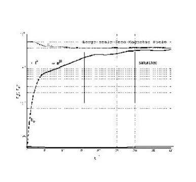
Figure 27: Evolution of kinetic energy ($E^{u}$) and magnetic energy $(E^{b})$ for initial weak, large-scale seed magnetic field. Initially $E^{b}$ grows as $t^{2}$, then exponentially, after which it saturates. Adopted from Chou Chou:num .

For the initial condition of type (b), initial growth of magnetic energy is determined by the eddy turnover time of the smallest scale of turbulence, as predicted by KA, and then by the eddy turnover time of inertial range modes (See Fig. 28); finally the growth saturates.

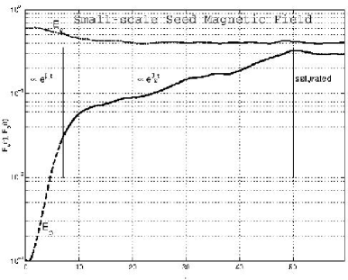
Figure 28: Evolution of kinetic energy ($E^{u}$) and magnetic energy $(E^{b})$ for initial weak, small-scale seed magnetic field. $E^{b}$exponentially, then it saturates. Adopted from Chou Chou:num .

When the initial seed magnetic energy is at narrow bandwidth of large wavenumbers, the magnetic energy quickly gets spread out, extending to both larger and smaller wavenumbers. The evolution of energy spectrum is shown in Fig. 29. In the early phase, the magnetic energy spectrum is proportional to $k^{3/2}$, confirming KA’s predictions. However, at a later time, the energy spectrum is very different, which is due to the dynamic aspect of dynamo.

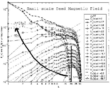
Figure 29: Magnetic and kinetic energy spectrum at various times. Initial seed magnetic field is concentrated at $k=20$. $E^{b}(k)\propto k^{3/2}$ for $2<t<10$, reminiscent of Kulsrud and Anderson’s predictions. It shifts to flatter and then to Kolmogorov-like spectrum at later time. Adopted from Chou Chou:num .

Recently Cho and Vishniac (CV) ChoVish:gene performed numerical simulation of nonhelical MHD turbulence and arrived at the following conclusion based on their numerical results. In our language, their results for large $r_{A}$ can be rephrased as (1) $\Pi_{u>}^{u<}\approx U^{3}$; (2) $\Pi_{(b<+b>)}^{u<}\approx UB^{2}$; (3) $\Pi_{b<}^{u<}\approx(U-cB)B^{2}$, where $U$ and $B$ are the large-scale velocity and magnetic field respectively, and $c$ is a constant. These results are somewhat consistent with the field-theoretic flux calculations of Verma MKV:MHD_Flux .

X.2.3 Brandenburg’s Calculations

Brandenburg Bran:Alpha performed direct numerical simulation of compressible MHD (Mach number around 0.1-0.3) on maximum grid of $128^{3}$. He applied kinetic energy and kinetic helicity forcing in the wavenumber band $(4.5,5.5)$. He obtained many interesting results, some of which are given below.

1. Magnetic helicity grows at small wavenumbers, but it has a negative sign. Brandenburg explains this phenomena by invoking conservation of magnetic helicity. For a closed or periodic system the net magnetic helicity is conserved, except for dissipation at small scales. Thus, for magnetic field to be helical, it must have equal amount of positive and negative helicity. The helicity at small scales will get destroyed by dissipation, while magnetic helicity at large scales will survive with negative sign.

2. Brandenburg computed the magnetic-helicity flux and found that to be positive. Note that injection of kinetic helicity induces a flux of magnetic-helicity (see Eq. [241]).

3. Brandenburg argued that most of the energy input to the large scale field is from scales near the forcing. He claimed the above process to be alpha-effect, not an inverse cascade (local). Now the built-up energy at large scales cascades to neighbouring scales by forward cascade ($k^{3/2}$ region). Once the large scale fields have grown, Kolmogorov’s direct cascade will take place. Above observations are illustrated in Fig 30.

   

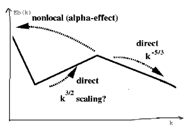
   Figure 30: Cascade processes of magnetic energy in Helical MHD turbulence. Adopted from Brandenburg Bran:Alpha .

Brandenburg has done further work on open boundaries, and applied these ideas to solar dynamo. For details, refer to review paper by Brandenburg Bran:rev_helicity . Verma MKV:MHD_Flux ; MKV:MHD_Helical has computed energy fluxes and shell-to-shell energy transfers in MHD turbulence using field-theoretic calculations. Below we show how Verma’s results are consistent with Brandenburg’s results.

X.2.4 Dynamo using Energy Fluxes

In Section VIII we discussed various energy fluxes and shell-to-shell energy transfer in MHD turbulence. Here we will apply those ideas to estimate the growth rate of magnetic energy. These calculations are based on homogeneous and isotropic turbulence, so the predictions made here are probably valid for galactic dynamo, or at small scales in solar and planetary dynamo.

Verma has calculated energy flux for both nonhelical and helical MHD. It has been shown in Section X.1.1 that when $E^{u}(k)>E^{b}(k)$, kinetic energy gets transferred to magnetic energy, hence turbulence is not steady. Now we compute the energy transfer rate to the large-scale magnetic field. In absence of helicity, the source of energy for the large-scale magnetic field is $\Pi_{b<}^{u<}$. When helicity is present, the fluxes $\Pi_{b<helical}^{b>}+\Pi_{b<helical}^{u>}$ provide additional energy to the large-scale magnetic field (see Sec. VIII). Hence, the growth rate of magnetic energy is

$$\frac{dE^{b}(t)}{dt}=\Pi_{b<}^{u<}+\Pi_{b<helical}^{b>}+\Pi_{b<helical}^{u>}$$ (264)

Since there is no external forcing for large-scale magnetic field, we assume

$$\Pi_{b<}^{u<}\approx\Pi_{b>}^{b<}+\Pi_{u>}^{b<}.$$

In typical astrophysical situations, magnetic and kinetic helicities are typically small, with negative magnetic helicity and positive kinetic helicity. For this combination of helicities, both the helical fluxes are negative, thus become a source of energy for the growth for large-scale magnetic field.

Since the magnetic energy starts with a small value (large $r_{A}$ limit), all the fluxes appearing in Eq. (264) are proportional to $r_{A}^{-1}$ [cf. Eqs. (231, 232)], i.e.,

$$\Pi_{b<}^{u<}+\Pi_{b<helical}^{b>}+\Pi_{b<helical}^{u>}=c\Pi\frac{E^{b}}{E^{u}}$$ (265)

where $E^{u}$ is the large-scale kinetic energy, $\Pi$ is the kinetic energy flux, and $c$ is the constant of order 1. Hence,

$$\frac{1}{\Pi}\frac{dE^{b}}{dt} \approx \frac{E^{b}}{E^{u}}$$ (266)

Using $E^{u}=K^{u}\Pi^{2/3}L^{2/3}$, where $L$ is the large length-scale of the system, we obtain

$$\frac{1}{\sqrt{E^{u}}E^{b}}\frac{dE^{b}}{dt}\approx\frac{1}{L(K^{u})^{3/2}}$$ (267)

We assume that $E^{u}$ does not change appreciably in the early phase. Therefore,

$$E^{b}(t)\approx E^{b}(0)\exp{\left(\frac{\sqrt{E^{u}}}{L(K^{u})^{3/2}}t\right)}$$ (268)

Hence, the magnetic energy grows exponentially in the early periods, and the time-scale of growth is of the order of $L(K^{u})^{3/2}/\sqrt{E^{u}}$, which is the large-scale eddy turnover time.

In Section VIII.1.3 we derived the following expression (Eq. [241]) for the flux of magnetic helicity:

$$\Pi_{H_{M}}(k_{0})=\frac{1}{k_{0}}\left(-dr_{M}+er_{K}\right),$$ (269)

where $r_{K}=H_{K}(k)/(kE^{u}(k))$, $r_{M}=kH_{M}(k)/E^{b}(k)$, and $d$ and $e$ are positive constants. When kinetic helicity is forced $(r_{K}>0)$ at forcing wavenumber, magnetic helicity flux will be positive. But the total magnetic helicity is conserved, so positive $H_{M}$ will flow to larger wavenumber, and negative $H_{M}$ will flow to smaller wavenumber. The negative $H_{M}$ ($r_{K}<0$) will further enhance the positive magnetic helicity flux, further increasing negative $H_{M}$ at lower wavenumbers. The above observation explains the numerical findings of Brandenburg Bran:Alpha discussed above.

The negative magnetic helicity described above contributes to the growth of magnetic energy. Note that for small wavenumber $H_{M}$ and $H_{K}$ have opposite sign, and according to formula (240) derived in Section VIII.1.3

$$\frac{dE^{b}}{dt}=ar_{M}^{2}-br_{M}r_{K},$$ (270)

($a$ and $b$ are positive constants) magnetic energy will grow. This result is consistent with the numerical simulation of Brandenburg Bran:Alpha and EDQNM calculation of Pouquet et al. Pouq:EDQNM . It is important to contrast the above equation with the growth equation of Pouquet et al. Pouq:EDQNM ) (cf. Eq. [263]) , and test which of the two better describes the dynamo. The direct numerical simulation of Pouquet and Patterson Pouq:num indicate that $H_{M}$ helps the growth of magnetic energy considerably, but that is not the case with $H_{K}$ alone. This numerical result is somewhat inconsistent with results of Pouquet et al. and others Pouq:EDQNM (Eq. [263]), but it fits better our formula (270) ($dE^{b}/dt=0$ if $r_{M}=0$). Hence, the formula (270) probably is a better model for the dynamically consistent dynamo. We need more careful numerical tests and analytic investigations to settle these issues.

In Section VIII we studied the shell-to-shell energy transfer in MHD turbulence assuming powerlaw energy spectrum for all of wavenumber space. Since magnetic helicity changes sign, and its spectrum does not follow a powerlaw, the above assumption is not realistic. However, some of the shell-to-shell energy transfer results are in tune with Brandenburg’s numerical results. For example, we found that helicity induces energy transfers across distant wavenumber shells, in the same lines as $\alpha$-effect. More detailed analytic calculation of shell-to-shell energy transfer is required to better understand dynamo mechanism.

X.2.5 Theoretical Dynamic Models

Field et al. Fiel:Dynamo and Chou Chou:theo constructed a theoretical dynamical model of dynamo. They use scale-separation and perturbative techniques to compute the effects of back-reaction of magnetic field on $\alpha$. Schekochihin et al. Maro:DynamoNlin and Blackman Blac:Rev_Dynamo discussed various models of nonlinear evolution and saturation for both small-scale and large-scale dynamo. Basu Basu:FieldthDynamo has applied field-theoretic methods to compute $\alpha$. For details refer to the original papers and review by Brandenburg and Subramanian Bran:PR .

In summary, dynamo theory has come a long way. Early calculations assumed kinematic approximations. For last fifteen years, there have been attempts to construct dynamic dynamo models, both numerically and theoretically. Role of magnetic and kinetic helicity is becoming clearer. Yet, we are far away from fully-consistent dynamo theory.

XI Intermittency in MHD Turbulence

The famous Kolmogorov’s turbulence model assumes a constant energy flux or dissipation rate at all scales, i. e., $\Pi(k)\sim\int dk\nu(k)k^{2}E(k)$ is independent of $k$. The renormalized viscosity $\nu(k)\sim k^{-4/3}$ and $E(k)\sim k^{-5/3}$ are consistent with the above assumption. Landau LandFlui:book pointed out that the dissipation rate, which is proportional to the square of vorticity, is singular and quite inhomogeneous. Thus Kolmogorov’s theory of turbulence needs modification. The above phenomena in which strong dissipation is localized both in time and space is called intermittency.

XI.1 Quantitative Measures of Intermittency

There are several quantitative measures of intermittency. Consider the increment of the velocity, or some other field, between two points separated by $\mathbf{l}$,

$$\delta\mathbf{u}(\mathbf{x,l})=\mathbf{u}(\mathbf{x}+\mathbf{l})-\mathbf{u}(\mathbf{x}).$$

The longitudinal component of $\delta\mathbf{u}(\mathbf{x,l})$ will be given by

$$\delta u_{||}(l)=\delta\mathbf{u}(\mathbf{x,l}).\mathbf{l}/l,$$

and the transverse component is $\delta u_{\perp}(l)=\delta\mathbf{u}(\mathbf{x,l})-\delta u_{||}(l)\mathbf{l}/l$. Here we have assumed homogeneity and isotropy for turbulence, so that the increment in velocities depend only on $l$, not on $\mathbf{x}$. Now we define longitudinal and transverse structure functions using

$$S^{(n)}(l)=\left\langle\left[\delta u_{||}(l)\right]^{n}\right\rangle,\,\,\,\,U^{(n)}(l)=\left\langle\left[\delta u_{\perp}(l)\right]^{n}\right\rangle$$

respectively. The structure function $S^{(n)}(l)$ is expected to have a power law behaviour for $l$ in the inertial range,

$$S^{(n)}(l)=a_{n}l^{\zeta_{n}},$$ (271)

where $a_{n}$ and $\zeta_{n}$ are universal numbers. The exponents $\zeta_{n}$ are called the intermittency exponent.

Moments and probability density function (pdf) are equivalent description of random variables. Note that if $P(\delta u_{||}(l))$ were gaussian, i. e.,

$$P(\delta u_{||}(l))=\frac{1}{\sigma_{r}\sqrt{{\pi}}}\exp{-\frac{(\delta u_{||}(l))^{2}}{\sigma_{r}^{2}}}$$

then, it is easy to verify that

$$\left\langle(\delta u_{||}(l))^{n}\right\rangle\propto\sigma_{r}^{n}.$$

Kolmogorov’s model of turbulence predicts that

$$\sigma_{r}\sim\epsilon^{1/3}l^{1/3},$$

For constant $\epsilon$, we obtain

$$S^{(n)}(l)\propto\epsilon^{n/3}l^{n/3}.$$

Systems with gaussian probability distribution or equivalently $S^{(n)}(l)\propto l^{cn}$ ($c=$ constant) are called non-intermittent system. For intermittent systems, the tails of pdf decays slower that gaussian, and could follow a powerlaw.

Structure function can be written in terms of local dissipation rate Obuk

$$\delta u_{l}\sim\epsilon_{l}^{1/3}l^{1/3}.$$

Kolmogorov Kolm:Intermittency introduced the refined similarity hypothesis relating structure function to $\epsilon_{l}$ as

$$S_{||}^{(n)}(l)=d_{n}\left\langle\epsilon_{l}^{n/3}\right\rangle l^{n/3}.$$

If

$$\left\langle\epsilon_{l}^{n}\right\rangle\sim l^{\mu_{n}},$$

then

$$\zeta_{n}=\frac{n}{3}+\mu_{n/3}.$$

Many researchers have attempted to model $\epsilon_{l}$.

In any numerical simulation or experiment, the powerlaw range is quite limited. However, when we plot $S^{(n)}(l)$ vs. $S^{(3)}(l)$, we obtain a much larger scaling range. This phenomena is called Extended self-similarity (ESS). Since, $S^{(3)}(l)\propto l$ K41b , $\zeta_{n}$ measured using Eq. (271) or ESS are expected to be the same.

There have been some ingenious attempts to theoretically compute the intermittency exponents (e.g., see series of papers by L’vov and Procaccia LvovProc:Intermittency ). Yet, this problem is unsolved. There are several phenomenological models. Even here, phenomenological models have been better developed for fluid turbulence than MHD turbulence. We will describe some of them in the following discussion, first for fluids and then for MHD turbulence.

XI.2 Results on Intermittency in Fluid Turbulence

In fluid turbulence, the pdf of velocity increment deviates from gaussian Fris:book . In experiments and simulations one finds that $\zeta_{n}$ vs. $n$ is a nonlinear function of $n$. Hence, fluid turbulence shows intermittency. Note that $\zeta_{2}\approx 0.71,$ which yields a correction of approximately 0.04 to Kolmogorov’s spectral index of 5/3. However, the correction for large $n$ is much more. See Frisch Fris:book for further details.

Remarkably, starting from Navier-Stokes equation, Kolmogorov K41b obtained an exact relation

$$S_{||}^{(3)}(l)=-\frac{4}{5}\epsilon l$$

under $\nu\rightarrow 0$ limit (also see Fris:book ; LandFlui:book ). Note that $\epsilon$ is the mean dissipation rate. Unfortunately, similar relationship could not be derived for other structure functions. In the following discussion we will discuss some of the prominent intermittency models for fluid turbulence.

XI.2.1 Kolmogorov’s log-normal model

Obukhov Obuk and Kolmogorov Kolm:Intermittency claimed that the dissipation rate in turbulent fluid is log-normal. As a consequence,

$$\zeta_{n}=\frac{n}{3}-\mu\frac{n(n-3)}{18},$$

where

$$\left\langle\epsilon(\mathbf{x})\epsilon(\mathbf{x+l})\right\rangle\sim l^{-\mu}.$$

Numerical simulations and experiments give $\mu\approx 0.2.$

The predictions of this model agree well with the experimental results up to $n\approx 10$, but fails for higher values of $n$. In Fig. 31 we have plotted the above $\zeta_{n}$ along with other model predictions given below.

Figure 31: Plots of $\zeta_{n}$vs. $n$ for various intermittency models in fluids and MHD. She-Leveque’s log-Poission model fits best with the experimental data in both fluid and MHD. For MHD turbulence, Kolmogorov-like models are in better agreement than KID’s like model.

XI.2.2 The $\beta-$model

Novikov and Stewart Novi and Frisch et al. Fris:Beta proposed that smaller scales in turbulent fluid is less space filling. In each step of the cascade an eddy $\delta u_{n}$ of scale $l_{n}$ splits into $2^{D}\beta$ eddies of scale $l_{n+1}=l_{n}/2$, where $D$ is the space dimensionality, and $\beta$ is a fixed parameter with $0<\beta\leq 1$. In this model

$$\zeta_{n}=\frac{n}{3}-\frac{\delta}{3}(n-3),$$

where $\beta=2^{-\delta}$.

Note that $\zeta_{n}$ is linear in $n$, and it does not match with experimental and numerical data for large $n$ (see Fig. 31).

XI.2.3 The Multifractal Models

Parisi and Frisch FrisPari developed a multifractal model of turbulence. Maneveau and Sreenivasan Sree1 constructed an intuitive model. Here the energy cascade rate $\epsilon_{l}$ is not distributed equally into smaller eddies, say, in each cascade it gets divided into $p\epsilon_{l}$ and $(1-p)\epsilon_{l}$. After several cascades, one finds that energy distribution is very skewed or intermittent. The intermittency exponent in this model is

$$\zeta_{n}=\left(\frac{n}{3}-1\right)D_{n}+1,$$

with

$$D_{n}=\log_{2}\left(p^{n}+(1-p)^{n}\right)^{1/(1-n)}.$$

For $p$ near 0.7, $\zeta_{n}$ fits quite well with the experimental data. The deficiency of this model is that it requires an adjustable parameter $p$. For more detailed discussion, refer to Stolovitzky and SreenivasanSree:RMP .

XI.2.4 The Log-Poisson Model

She and Leveque SheLeve proposed a model involving a hierarchy of fluctuating structures associated with the vortex filament. In their model

$$\zeta_{n}=\frac{n}{3}(1-x)+C_{0}\left(1-\beta^{n/3}\right)$$ (272)

where $C_{0}$ is co-dimension of the dissipative eddies, and $x$ and $\beta$ are parameters connected by

$$C_{0}=\frac{x}{1-\beta}$$ (273)

(see Biskamp BiskTurb:book for details; also see Politano and Pouquet Poli:Intermittency ). For Kolmogorov scaling, $x=\beta=2/3$. In hydrodynamic turbulence, the dissipative eddies are vortex filaments, i.e., one-dimensional structures. Therefore, the co-dimension is $C_{0}=2$. Hence, for fluid turbulence

$$\zeta_{n}^{SL}=\frac{n}{9}+2\left[1-\left(\frac{2}{3}\right)^{n/3}\right].$$ (274)

The above prediction fits remarkably well with experimental results. All the above functions have been plotted in Fig. 31 for comparison.

After the above introductory discussion on intermittency in fluid turbulence, we move on to intermittency in MHD turbulence.

XI.3 Results on Intermittency in MHD Turbulence

In MHD turbulence, the pdf of increment of velocity, magnetic, and Elsässer variables are all nongaussian. The $\zeta_{n}$ vs. $n$ is a nonlinear function of $n$, hence MHD turbulence also exhibits intermittency. The theoretical and phenomenological understanding of intermittency in MHD turbulence is more uncertain than that in fluid turbulence because the nature of energy dissipation rates in MHD turbulence is still quite obscure.

Following the similar lines as Kolmogorov K41b , Politano and Pouquet Poli:S3exact derived an exact relationship:

$$\left\langle\delta z_{||}^{\mp}\delta z_{i}^{\pm}\delta z_{i}^{\pm}\right\rangle=-\frac{4}{3}\epsilon^{\pm}l.$$

This result is consistent with Kolmogorov-like model (Eq. [103]) that

$$\delta z_{l}^{\pm}\sim\left(\epsilon^{\pm}\right)^{2/3}\left(\epsilon^{\mp}\right)^{-1/3}l^{1/3}.$$

There are more than one set of exponents in MHD because of presence of more number of variables. For $\mathbf{z}^{\pm}$ variables we have

$$S_{n}^{\pm}(l)=\left\langle\left|\delta z_{l}^{\pm}\right|^{n}\right\rangle\sim l^{\zeta_{n}^{\pm}}.$$

In the following, we will discuss Log-Poission model and numerical results on intermittency in MHD turbulence.

XI.3.1 The log-Poisson model

Politano and Pouquet Poli:Intermittency extended She and Leveque’s formula (272) to MHD turbulence. They argued that smallest eddies in fully developed MHD turbulence are micro-current sheets, hence the codimension will be $C_{0}=1$. Kolmogorov’s scaling yields $x=2/3$ and $\beta=1/3$. Therefore

$$\zeta_{n}^{MHD}=\frac{n}{9}+1-\left(\frac{1}{3}\right)^{n/3}.$$

If KID’s scaling were to hold for MHD, then $x=1/2$ and $\beta=1/2$. Consequently,

$$\zeta_{n}^{KID}=-\frac{n}{2}+1-\left(\frac{1}{2}\right)^{n/3}.$$

For details refer to Biskamp BiskTurb:book . Now we compare these predictions with the numerical results.

XI.3.2 Numerical Results

Biskamp and Müller Bisk:Kolm2 have computed the exponents $\zeta_{n}^{\pm}$ for 3D MHD, and they are shown in Fig. 32.

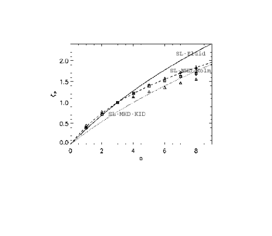
Figure 32: Numerically computed intermittency exponents $\zeta_{n}^{+}$(diamond) and $\zeta_{n}^{-}$ (square) for 3D MHD turbulence, and $\zeta_{n}^{+}/\zeta_{3}^{+}$ (triangle) for 2D MHD turbulence. The numerical values matches quite well with the She-Leveque model based on Kolmogorov-like spectrum (dashed line). Adopted from Biskamp and Müller Bisk:Kolm2 .

In the same plot, $\zeta_{n}^{MHD}$and $\zeta_{n}^{KID}$ have also been plotted. Clearly, $\zeta_{n}^{MHD}$ agrees very well with 3D MHD numerical data. This again shows that Kolmogorov-like phenomenology models the dynamics of MHD turbulence better that KID’s phenomenology. In Fig. 32 She-Leveque’s predictions for fluid (solid line) and KID’s model (dotted line) are also shown for reference. 2D MHD appears to be more intermittent than 3D MHD. A point to note that the plots of Figs. 31, 32 are for small cross helicity ($\sigma_{c}\rightarrow 0$); the equality of $\zeta_{n}^{+}$ and $\zeta_{n}^{-}$ may not hold for higher cross helicity.

Müller et al. Mull:IntermittencyB0 numerically computed the intermittency exponents in the presence of mean magnetic field. They found that a mean magnetic field reduces the parallel-field dynamics, while in the perpendicular direction a gradual transition toward 2D MHD turbulence is observed.

Biskamp and Schwarz Bisk:2D computed the intermittency exponents for 2D MHD turbulence (see Table III of Biskamp and Schwarz Bisk:2D ). The exponents are much lower than $\zeta_{n}^{MHD}$. The exponent $\zeta_{2}$ is close to 0.5, which prompted Biskamp and Schwarz to infer that 2D MHD follows KID’s phenomenology with $E(k)\sim k^{-\zeta_{2}-1}\sim k^{-3/2}$ power spectrum. However, $\zeta_{4}$ is much below 1, which makes the claim less certain. Earlier, using flux analysis Verma et al. MKV:MHD_Simulation had shown that Kolmogorov-like phenomenology is a better model for 2D MHD than KID’s phenomenology (see Section VI). Hence, Biskamp and Schwarz Bisk:2D and Verma et al.’s MKV:MHD_Simulation conclusions appear contradictory. It may be possible that 2D MHD turbulence is highly intermittent, with 5/3 exponent still applicable. In any case, further work is required to clarify these issues. Refer to Verma et al. MKV:Bisk_Comment and Biskamp Bisk:MKV_Comment for further details.

Basu et al. Basu:Intermittency numerically computed the intermittency exponents for velocity and magnetic fields. They showed that $\zeta^{b}>\zeta^{\pm}>\zeta^{u}$, i.e., magnetic field is more intermittent than the velocity field. They also find that $\zeta^{b}\approx\zeta^{SL}$. For theoretical arguments regarding $\zeta^{u}$ and $\zeta^{b}$ we refer to Eq. (214), which implies that

$$\delta u_{l} \sim \left(\Pi^{u}\right)^{1/3}l^{1/3}$$

$$\delta b_{l} \sim \left(\Pi^{b}\right)^{1/3}l^{1/3},$$

where $\Pi^{u}=\Pi_{u>}^{u<}+\Pi_{b>}^{u<}$ is the total kinetic energy flux, and $\Pi^{b}=\Pi_{b>}^{b<}+\Pi_{u>}^{b<}$ is the total magnetic energy flux. Clearly,

$$S^{u(n)}(l) = \left\langle\left(\delta u_{l}\right)^{n}\right\rangle=\left\langle\left(\Pi^{u}\right)^{n/3}\right\rangle l^{n/3}\sim l^{\zeta_{n}^{u}}$$

$$S^{b(n)}(l) = \left\langle\left(\delta b_{l}\right)^{n}\right\rangle=\left\langle\left(\Pi^{b}\right)^{n/3}\right\rangle l^{n/3}\sim l^{\zeta_{n}^{b}}.$$

Hence, $\zeta^{u}$ and $\zeta^{b}$ depend on the small-scale properties of $\Pi^{u}$ and $\Pi^{b}$. From the numerical results of Basu et al. Basu:Intermittency it appears that $\Pi^{b}$ is more intermittent that $\Pi^{u}$. Note that Basu et al.’s result was derived from magnetically dominated run, So we need to test the above hypothesis for various ratios of kinetic and magnetic energies.

Some of the earlier work on intermittency in MHD turbulence has been done by Carbone Carb:IntermittencyFirst . His work is based on KID’s model, and he alludes that the spectral index of solar wind is close to 1.7 because of intermittency correction of approximately 0.2 over 3/2. There is also an extensive investigation of intermittency in solar wind data. Refer to Burlaga Burl , Marsch and Tu MarsTu:Nongaussian , and Tu et al. MarsTu:StructureFn .

It is evident from the above discussion that physical understanding of intermittency is quite weak. We need to better understand dissipation rates in MHD turbulence. With these remarks, we close our discussion on intermittency.

XII Miscellaneous Topics

In this section we will briefly discuss the following topics connected to the spectral theory of MHD turbulence: (a) Large-Eddy simulations of MHD Turbulence, (b) Energy decay of MHD turbulence, (c) Shell model of MHD turbulence, and (d) Compressible Turbulence.

XII.1 Large-Eddy Simulations (LES) of MHD Turbulence

Basic idea of LES is to resolve only the large scales of turbulent flow. The effect of smaller scale interactions are modeled appropriately using the existing theories. Let $u_{K}^{<}$ and $b_{K}^{<}$ represent the filtered fields at filter width of $l$. The filtered MHD equations are

$$\frac{\partial\mathbf{u}^{<}}{\partial t} = -\nabla\cdot\left(\mathbf{u}^{<}\mathbf{u}^{<}-\mathbf{b}^{<}\mathbf{b}^{<}+\mathbf{\tau}^{u}\right)-\nabla p^{<}+\nu\nabla^{2}\mathbf{u}^{<}$$

$$\frac{\partial\mathbf{b}^{<}}{\partial t} = -\nabla\cdot\left(\mathbf{u}^{<}\mathbf{b}^{<}-\mathbf{b}^{<}\mathbf{u}^{<}+\mathbf{\tau}^{b}\right)+\nu\nabla^{2}\mathbf{u}^{<}$$

$$\nabla\cdot\mathbf{u}^{<} = \nabla\cdot\mathbf{b}^{<}=0,$$

where $\mathbf{\tau}^{u}=(\mathbf{uu})^{<}-\mathbf{u}^{<}\mathbf{u}^{<}-(\mathbf{bb})^{<}+\mathbf{b}^{<}\mathbf{b}^{<}$, and $\mathbf{\tau}^{b}=(\mathbf{ub})^{<}-\mathbf{u}^{<}\mathbf{b}^{<}-(\mathbf{bu})^{<}+\mathbf{b}^{<}\mathbf{u}^{<}$ are the filtered-scale stress tensors. Main task in LES is to model these tensors. A class of models assume that MullCara_pop1 ; MullCara_pop2

$$\mathbf{\tau}^{u}=-2\nu_{t}\mathbf{S}^{<},\,\,\,\,\,\mathbf{S}^{<}=\left(\nabla\mathbf{u}^{<}+[\nabla\mathbf{u}^{<}]^{T}\right)/2,$$

$$\mathbf{\tau}^{b}=-2\eta_{t}\mathbf{J}^{<},\,\,\,\,\,\mathbf{J}^{<}=\left(\nabla\mathbf{b}^{<}+[\nabla\mathbf{b}^{<}]^{T}\right)/2,$$

where “$T$” denotes the transposed matrix, and $\nu_{t}$ and $\eta_{t}$ are the eddy-viscosity and eddy-resistivity respectively. Agullo et al. MullCara_pop1 and Müller and Carati MullCara_pop2 prescribed $\nu_{t}$ and $\eta_{t}$ using two different models $M_{1}$ and $M_{2}$:

$$M_{1}: \nu_{t}=C_{1}(t)l^{4/3}, \eta_{t}=D_{1}(t)l^{4/3},$$

$$M_{2}: \nu_{t}=C_{2}(t)l^{2}(2\mathbf{S^{<}}:\mathbf{S^{<}})^{1/2}, \eta_{t}=D_{2}(t)l^{2}|\mathbf{j}^{<}|.$$

Both models contain two unknown parameters $C_{i}$ and $D_{i}$. Agullo et al. MullCara_pop1 and Müller and Carati MullCara_pop2 determined these parameters using dynamic LES, in which a test filter is used Germ . After determining $\nu_{t}$ and $\eta_{t}$, the velocity and magnetic fields were updated using DNS. Their evolution of kinetic and magnetic energy using Models $M_{1}$ and $M_{2}$ agree quite well with DNS. The decay of the magnetic energy in DNS and $M_{1,2}$ are quite close, but there is a slight discrepancy. Note that $M_{0}:\mathbf{\tau}^{u,b}=0$ fares quite badly.

We Shis employ DNS to MHD equations, but viscosity and resistivity are replaced by renormalized viscosity and renormalized resistivity given below:

$$\nu_{r}(k_{C}) = (K^{u})^{1/2}\Pi^{1/3}k_{C}^{-4/3}\nu^{*}$$ (275)

$$\eta_{r}(k_{C}) = (K^{u})^{1/2}\Pi^{1/3}k_{C}^{-4/3}\eta^{*}.$$ (276)

Here $K^{u}$ is Kolmogorov’s constant for MHD, $\Pi$ is the total energy flux, and $\nu^{*},\eta^{*}$ are the renormalized parameters. The parameters $\nu^{*},\eta^{*}$, and $K^{u}$ depend on the Alfvén ratio $r_{A}$. In our decaying MHD turbulence simulation, we start with unit total energy and $r_{A}=100.0$. The ratio of magnetic to kinetic energy grows as a function of time, as expected. Therefore, we need to compute the renormalized parameters for various values of $r_{A}$. The energy cascade rates are computed following the method described in Section VI. We take $\nu_{r}(k_{C})$ and $\eta_{r}(k_{C})$ from Eqs. (275, 276). The energy flux $\Pi$ changes with time; we compute $\Pi$ dynamically every $0.01$ time-unit. We carried out LES for MHD up to 25 nondimensional time units. McComb et al. McCo:LES had done a similar LES calculation.

The evolution of kinetic energy using LES is quite close to that using DNS. However, the evolution of magnetic energy does not match very well. Comparatively, LES of Agullo et al. MullCara_pop1 and Müller and Carati MullCara_pop2 yield a better fit to the temporal evolution of magnetic energy. Hence, refinements are required in our modelling.

In summary, LES of MHD turbulence is in its infancy, and More work is required in modelling of eddy-viscosity and resistivity.

XII.2 Energy Decay of MHD Turbulence

The models of energy decay in MHD turbulence are motivated by the decay laws of fluid turbulence. In these models, the energy loss is due to Kolmogorov’s energy flux. In addition, conservation laws are used to close the equation. Biskamp and Müller Bisk:Kolm2 first proposed that

$$E^{b}l_{0}=H_{M},$$ (277)

where $l_{0}$ is the integral scale, $E^{b}$ is the total magnetic energy, and $H_{M}$ is magnetic helicity. The corresponding equation for fluid turbulence is $EL^{s+1}=const$, with $s=4$. Assuming advection term to be the dominant nonlinearity for energy flux, Biskamp and Mülller suggested that the dissipation rate $\epsilon$ is

$$\epsilon=-\frac{dE}{dt}\sim\mathbf{u}\cdot\nabla E\sim\left(E^{u}\right)^{1/2}\frac{E}{l_{0}}.$$

A substitution of $l_{0}$ of Eq. (277) into the above equation yields

$$\frac{E^{5/2}}{\epsilon H_{M}}\frac{r_{A}}{(1+r_{A})^{3/2}}=const.$$

This phenomenological formula was found to be in very good agreement with numerical result. Alfvén ratio $r_{A}$ itself is varies with time; Biskamp and Müller numerically found its variation to be $r_{A}\approx 1.5(E/H_{M})$. Using this result and taking the limit $r_{A}\ll 1$, they obtained

$$-\frac{dE}{dt}\approx 0.5\frac{E^{3}}{H^{3/2}}$$

with the similarity solution $E\sim t^{-1/2}$. The relationship $r_{A}\approx 1.5(E/H_{M})$ yields $E^{u}\sim(E^{b})^{2}\sim t^{-1}$. For finite $r_{A}$, the evolution is expected to be somewhat steeper.

For nonhelical MHD ($H_{M}=0$), Biskamp and Müller found a different decay law

$$\frac{dE}{dt}E^{-2}=const$$

yielding $E\sim t^{-1}$; this result was verified in numerical simulations. Note that all the above arguments are valid for zero or vanishing cross helicity. When cross helicity is finite, it decays with a finite rate. Galtier et al. Galt:Decay reached to the similar conclusions as Biskamp. Note that similar arguments for fluid turbulence shows that kinetic energy decays as $t^{-10/7}$.

In the light of current results on evolution of kinetic and magnetic energy discussed in Section VIII.2, some new deductions can made regarding the energy evolution in MHD turbulence. Since the energy fluxes $\Pi^{\pm}$ are not coupled (see Fig. 6), we expect $E^{\pm}$ to decay in the same way as fluid turbulence. However, the evolution of kinetic and magnetic energy is more complex because of cross transfers of energy between velocity and magnetic fields (see Fig. 5). Their evolution in nonhelical MHD could be modelled as

$$\frac{dE^{b}}{dt} = \Pi_{b<}^{u<}-\Pi^{b},$$

$$\frac{dE^{u}}{dt} = \Pi_{u<}^{b<}-\Pi^{u}.$$

In kinematic regime ($E^{u}\gg E^{b}$), $E^{b}$ grows exponentially (dynamo) due to $\Pi_{b<}^{u<}$, and $E^{u}$ should decay as in fluid turbulence. However, in magnetic regime ($E^{b}\gg E^{u}$), magnetic energy should decay faster than kinetic energy due to positive $\Pi_{u<}^{b<}$. Since $E^{u}$ and $E^{b}$ are equipartitioned in the asymptotic state, it may be possible that $\Pi_{b<}^{u<}=|E^{u}-E^{b}|^{h}$. Using these ideas, we may get further insights into the physics of decay in MHD turbulence.

XII.3 Shell Models of MHD Turbulence

Shell models of turbulence were introduced as an attempt to solve hydrodynamic equations using much fewer degrees of freedom. In these models, one variable is used to represent all the modes in wavenumber shell $(k_{n},k_{n+1})$. The shell radius is given by $k_{n}=k_{0}s^{n}$ with $s$ as a parameter, typically taken to be 2. The coupling between shells is local with constraints of preserving conserved quantities. One type of shell-model for MHD turbulence is given below Fric :

$$\left(\frac{d}{dt}+\nu k^{2}\right)U_{n} = ik_{n}[(U_{n+1}^{*}U_{n+2}^{*}-B_{n+1}^{*}B_{n+2}^{*})-\frac{\epsilon}{2}(U_{n-1}^{*}U_{n+1}^{*}-B_{n-1}^{*}B_{n+1}^{*})$$ (278)

$$-\frac{(1-\epsilon)}{4}(U_{n-2}^{*}U_{n-1}^{*}-B_{n-2}^{*}B_{n-1}^{*})]+f_{n}$$

$$\left(\frac{d}{dt}+\eta k^{2}\right)B_{n} = ik_{n}[(1-\epsilon-\epsilon_{m})(U_{n+1}^{*}B_{n+2}^{*}-B_{n+1}^{*}U_{n+2}^{*})+\frac{\epsilon_{m}}{2}(U_{n-1}^{*}B_{n+1}^{*}-B_{n-1}^{*}U_{n+1}^{*})$$ (279)

$$\frac{(1-\epsilon_{m})}{4}(U_{n-2}^{*}B_{n-1}^{*}-B_{n-2}^{*}U_{n-1}^{*})]+g_{n},$$

where $f_{n}$ and $g_{n}$ are kinetic and magnetic forcing respectively. The above equations conserve total energy and cross helicity for any $\epsilon_{m}$. However, conservation of the third integral imposes condition on $\epsilon^{\prime}$s. In 3D, this integral is

$$H_{M}=\sum_{n}(-1)^{n}k_{n}^{-1}|B_{n}|^{2},$$

which is conserved if $\epsilon=1/2$ and $\epsilon_{m}=1/3$. in 2D, the choice of $\epsilon=5/4$ and $\epsilon_{m}=-1/3$ leads to conservation of

$$a=\sum_{n}k_{n}^{-2}|B_{n}|^{2}.$$

Frick and Sokoloff Fric numerically solved Eqs. (278, 279) with 30 shells ($-4\leq n\leq 27$). The system was forced near the $n=0$ shell. The time integration was done using fourth-order Runge-Kutta method. Frick and Sokoloff studied energy spectrum, fluxes, and the structure functions. They obtained Kolmogorov-like energy spectrum (5/3) for nonAlfvénic MHD ($\sigma_{c}\approx 0$); this state is independent of magnetic helicity $H_{M}$. However, when the magnetic and velocity fields are correlated, Kolmogorov state is not established, and the result depends on the magnetic helicity. High level of $H_{M}$ suppresses any cascade of energy, and KID’s spectra was obtained.

Frick and Sokoloff Fric and Basu et al. Basu:Intermittency studied the structure functions of MHD. They found that intermittency in MHD turbulence is slightly higher than in the hydrodynamic case, and the level of intermittency for the magnetic field is slightly higher than the velocity field. Biskamp Bisk:cascade has studied the effect of mean magnetic field using Shell model. For reference, Gloaguen et al. Pouq:Shell constructed one of the first shell models for MHD turbulence.

Shell models are based on an assumption of local energy transfer. This assumption appears to be suspect in the light of our results on shell-to-shell energy transfer described in VIII.2, where we showed that there are significant amount of nonlocal energy transfer in MHD turbulence, specially in presence of magnetic helicity. This issue requires a closer look.

XII.4 Compressible Turbulence

Terrestrial MHD plasmas are incompressible because plasma velocities are typically much smaller compared to sound speed or Alfvén speed. However, astrophysical plasmas are typically compressible. Currently the energy spectrum of incompressible (infinite sound speed) and fully-compressible (zero sound speed) turbulence are reasonably well understood. Fully compressible fluid is described by Burgers equation

$$\frac{\partial\mathbf{u}}{\partial t}+(\mathbf{u}\cdot\nabla)\mathbf{u}=\nu\nabla^{2}\mathbf{u}.$$

for which shocks are exact solution in 1D under $\nu\rightarrow 0$ limit. It can be easily shown that $E(k)\sim k^{-2}$ and intermittency exponents $\zeta_{q}=1$ for $q>1$. Shocks are present in higher dimensions as well, and the spectral index is expected to be 2. Fully-compressible MHD turbulence, modelled by generalized Burgers equation GaltPouq:Compressible , also show shocks. For properties of shocks, refer to Biskamp BiskTurb:book and Priest Prie:book . For the other limiting case, incompressible fluid turbulence as well as MHD turbulence are well described by Kolmogorov’s theory of turbulence. The difficulty is with finite Mach number.

The velocity in compressible fluids is decomposed into compressible part $\mathbf{u}^{c}$ and solenoidal part $\mathbf{u}^{s}$. In Fourier space, $\mathbf{u}^{s}$ is perpendicular to $\mathbf{k}$, and $\mathbf{u}^{c}$ is parallel to $\mathbf{k}$. Corresponding to these fields, we have solenoidal and compressive velocity spectrum, $E^{s}(k)$ and $E^{c}(k)$. Porter et al. Port:PRL showed that in the supersonic turbulence ($Ma>1$) , $E^{c}(k)\sim k^{-2}$, which is similar to the spectrum in Burgers turbulence. However for subsonic turbulence ($Ma<1$), both $E^{c}$ and $E^{s}$ have 5/3 spectral index.

Pressure spectrum is defined using $\left\langle p^{2}\right\rangle=\int E^{P}(k)dk$. Assuming 5/3 spectrum for velocity and using $p_{k}\sim\rho_{0}u_{k}^{2}$, Batchelor Batc:Pressure , and Monin and Yaglom MoniYagl2:book obtained

$$\frac{1}{\rho_{0}^{2}}E^{P}(k)\sim\epsilon^{4/3}k^{-7/3}.$$

The above law is expected to be valid for subsonic flows. For polytropic flows $p\sim\rho^{\gamma}$ , or

$$\delta\rho=C_{s}^{2}\delta\rho,$$

using which we can immediately derive the density spectrum for subsonic flows

$$N^{\rho}(k)=\epsilon^{4/3}C_{s}^{-4}k^{-7/3}.$$

Note that $\left\langle\rho^{2}\right\rangle=\int N^{\rho}(k)dk$.

For nearly incompressible MHD turbulence Montgomery et al. Mont:Density argued that $E^{P}(k)\sim N^{\rho}(k)\sim k^{-5/3}$. Their argument is based on quasi-normal model. For detail refer to Montgomery et al. Mont:Density and Zank and Matthaeus Zank:Compress_PoF ; Zank:Compress_PRL . Lithwick and Goldreich Gold:Compress also obtained Kolmogorov’s spectrum for the density fluctuations in the ionized interstellar medium. They calculated the above density spectrum by extending the theory of incompressible MHD given by Goldreich and Sridhar Srid1 ; Srid2 . Cho and Lazarian Cho:Compressible found similar results in their computer simulation.

It is interesting to note that Burgers equation is local in real space, contrary to incompressible turbulence which is nonlocal in real space. Also, “mode-to-mode” energy transfer formulas of Dar et al. Dar:flux cannot be applied to Burgers equation because $\nabla\cdot\mathbf{u}=0$ is not applicable to Burgers equation. We need some kind of generalized theory which will continuously vary the energy spectrum as we change the Mach number.

XIII Conclusions and Future Directions

Here we summarize the main results in statistical theory of MHD turbulence. In this paper, we focussed on the energy spectrum, fluxes, and the shell-to-shell energy transfers in homogeneous turbulence. When the mean magnetic field is applied, turbulence is naturally anisotropic. When the mean magnetic field is much greater that fluctuations (weak turbulence), the energy cascade is planar, perpendicular to the mean magnetic field; In this limit Galtiers et al. Galt:Weak showed that

$$E_{1,2}(k_{\perp})\sim\left(\Pi B_{0}\right)^{1/2}k_{||}^{1/2}k_{\perp}^{-2}.$$ (280)

When the fluctuations become comparable to the mean magnetic field (strong turbulence), Goldreich and Sridhar Srid1 ; Srid2 showed that $E(k)\sim k_{\perp}^{-5/3}$, thus establishing Kolmogorov-like dynamics for MHD turbulence. Verma MKV:B0_RG showed that the nonlinear evolution of Alfvén waves are affected by “effective mean magnetic field”, and showed that Kolmogorov’s 5/3 powerlaw is a valid spectrum for MHD turbulence. The effective mean-magnetic field turns out to be local ($k$-dependent) field, and can be interpreted as the field due to the next largest eddy. The above theoretical result is seen in the numerical simulation of Cho et al. ChoVish:localB . The renormalization group calculations (e. g., Verma MKV:MHD_RG ) also favor Kolmogorov’s 5/3 energy spectrum for MHD turbulence. All the above results have been discovered in the last ten years.

Let us contrast the above conclusions with the earlier results of Kraichnan Krai:65 and Iroshnikov Iros where effective time-scale is determined by the mean magnetic field $B_{0}$, and the energy spectrum is $k^{-3/2}$. Kraichnan’s and Iroshnikov’s phenomenology is weak turbulence theory under isotropic situations. This is contradictory because strong mean magnetic field will create anisotropy. This is why 3/2 theory is inapplicable to MHD turbulence.

Recently studied energy fluxes and shell-to-shell energy transfers in MHD turbulence are providing important insights into the energy exchange between velocity and magnetic fields, and also among various scales. These calculations have been done using “mode-to-mode” energy transfers in MHD triads. For 3D nonhelical flows ($H_{M}=H_{K}=0$), all the fluxes $u$-to-$u$, $u$-to-$b$, $b$-to-$u$, $b$-to-$b$ are positive except $b$-to-$u$, which is negative for large Alfvén ratio. In kinetic-energy dominated regime, kinetic energy flows to magnetic energy, and the reverse happens in magnetic-energy dominated regime. Hence, steady-state situation is possible only when $E^{u}\approx E^{b}$; we believe this to be the reason for the equipartition of kinetic and magnetic energy in MHD turbulence. The shell-to-shell energy transfer also suggests that nonhelical transfers are local. The $u$-to-$u$ and $b$-to-$b$ transfers are forward, but $u$-to-$b$ and $b$-to-$u$ are somewhat complex. Helicity induces inverse cascade of magnetic energy, but their magnitude is smaller than the nonhelical counterparts for small magnetic and kinetic helicities, which is typical. We also find a forward cascade for magnetic helicity.

Many of the above analytical work have been motivated by the clues obtained from numerical simulations, e. g., Bisk:Kolm1 ; Bisk:Kolm2 ; MKV:MHD_Simulation ; Dar:flux ; Maro:Simulation ; Chou:num . High resolution simulations, which can test spectrum as well as energy fluxes, have been made possible by recent powerful computers. In turbulence research, numerical simulations have become synonymous with experiments. Similarly, observational results from the solar wind data have been very useful in understanding the dynamics of MHD turbulence.

Amplification of magnetic field in MHD turbulence, commonly known as dynamo, has been of interest for almost a century. Earlier theories were of kinematic origin where given velocity spectrum induces growth of magnetic field, but the magnetic field cannot affect the velocity field. In the last ten years, there have been a surge of attempts to solve the full MHD equation including the back-reaction of the magnetic field to the velocity field. Pouquet et al. Pouq:EDQNM performed EDQNM calculations and showed that “residual helicity” (difference of kinetic helicity and magnetic helicity) induces growth of large-scale magnetic field. Some of the recent models are motivated by the numerical results. Brandenburg Bran:Alpha finds that kinetic helicity induces growth of negative magnetic helicity at large-scales, which in turn enhances the large-scale magnetic field. Chou Chou:num has shown growth of large-scale magnetic field with small-scale or large-scale seed magnetic field. Verma’s MKV:MHD_Helical analytical findings are in agreement with the the above mentioned numerical results. Field et al. Fiel:Dynamo , Chou Chou:theo , Schekochihin et al. Maro:DynamoNlin and Blackman Blac:Rev_Dynamo have constructed theoretical models of dynamics dynamo, and studied their nonlinear evolution and saturation mechanisms.

Intermittency exponents have been computed numerically by Müller and Biskamp Bisk:Kolm2 and others. Generalized She and Leveque’s SheLeve theoretical model based on log-Poisson process fits quite well with the numerical data. Note however that theoretical calculation of intermittency exponents from the first principles is still alluding turbulence researchers.

There are many unanswered questions in MHD turbulence. We list some of them here:

1. Goldreich and Sridhar’s Srid2 argument for 5/3 spectral index for strong MHD turbulence is semi-phenomenological. Generalization of Verma’s field-theoretic calculation for mean magnetic field MKV:B0_RG to anisotropic situations will be very useful. It will help us in quantifying the effects of mean magnetic field on energy fluxes etc.

2. Effects of magnetic and kinetic helicity on energy spectrum and fluxes is known only partially through numerical simulations and absolute-equilibrium theories.

3. Good understanding of compressible fluid and MHD is lacking. Theoretical studies of coupling of solenoidal, compressible, pressure modes etc. will advance our understanding in this area.

4. There are only a couple of large-eddy simulations (LES) of MHD turbulence, and they are not completely satisfactory. Considering the importance of LES in modeling large-scale practical systems, e.g., Tokomak flows, dynamo etc., further investigation of LES of MHD is required.

5. Application of field-theoretic calculation of MHD turbulence to electron magnetohydrodynamics Bisk:EMHD , active scalar Ruiz:Scalar , drift wave turbulence Driftwave etc. could help us in better understanding of these models.

6. Role of turbulence in corona heating, accretion disks, and other astrophysical objects are active area of research.

With these remarks we conclude our review.

Appendix A Fourier Series vs. Fourier Transform for Turbulent Flows

In statistical theory turbulence we typically assume the flow field to be homogeneous. Therefore, Fourier transform is not applicable to these flows in strict sense. However, we can define these quantities by taking limits carefully. This issue has been discussed by Batchelor BatcTurb:book and McComb McCo:book . We briefly discuss them here because they form the basis of the whole paper.

A periodic function $\mathbf{u}(\mathbf{x})$ in box $L^{d}$ can be expanded using Fourier series as following:

$$\mathbf{u}\left(\mathbf{x}\right) = \sum\hat{\mathbf{u}}\left(\mathbf{k}\right)\exp\left(i\mathbf{k\cdot x}\right),$$

$$\mathbf{\hat{u}(k}) = \frac{1}{L^{d}}\int d\mathbf{xu}\left(\mathbf{x}\right)\exp\left(-i\mathbf{k\cdot x}\right),$$

where $d$ is the space dimensionality. When we take the limit $L\rightarrow\infty$, we obtain Fourier transform. Using $\mathbf{u}(\mathbf{k})=\mathbf{\hat{\mathbf{u}}}(\mathbf{k})L^{d}$, it can be easily shown that

$$\mathbf{u}\left(\mathbf{x}\right) = \int\frac{d\mathbf{k}}{(2\pi)^{d}}\mathbf{u}\left(\mathbf{k}\right)\exp\left(i\mathbf{k\cdot x}\right),$$

$$\mathbf{u}(\mathbf{k}) = \int d\mathbf{xu}\left(\mathbf{x}\right)\exp\left(-i\mathbf{k\cdot x}\right),$$

with integrals performed over the whole space. Note however that Fourier transform (integral converges) makes sense when $u(x)$ vanishes as $|x|\rightarrow\infty$, which is not the case for homogeneous flows. However, correlations defined below are sensible quantities. Using the above equations, we find that

$$\left\langle u_{i}(\mathbf{k})u_{j}(\mathbf{k^{\prime}})\right\rangle = \int d\mathbf{x}d\mathbf{x^{\prime}}\left\langle u_{i}(\mathbf{x})u_{j}(\mathbf{x^{\prime}})\right\rangle\exp-i(\mathbf{k}\dot{\cdot\mathbf{x}+\mathbf{k^{\prime}}\cdot\mathbf{x^{\prime}})}$$ (281)

$$= \int d\mathbf{r}C_{ij}(\mathbf{r})\exp-i\mathbf{k}\cdot\mathbf{r}\int d\mathbf{x}\exp-i(\mathbf{k}\dot{+\mathbf{k^{\prime})}\cdot\mathbf{x}}$$

$$= C_{ij}(\mathbf{k})(2\pi)^{d}\delta(\mathbf{k+k^{\prime}})$$

We have used the fact that $\delta(\mathbf{k})\approx L^{d}/(2\pi)^{d}$. The above equation holds the key. In experiments we measure correlation function $C(\mathbf{r})$ which is finite and decays with increasing $r$, hence spectra $C(\mathbf{k})$ is well defined. Now energy spectrum as well as total energy can be written in terms of $C(\mathbf{k})$ as the following:

$$\left\langle u^{2}\right\rangle=\frac{1}{L^{d}}\int d\mathbf{x}u^{2}=\sum_{\mathbf{k}}\left|\mathbf{\hat{u}(k)}\right|^{2} = \frac{1}{L^{d}}\int\frac{d\mathbf{k}}{(2\pi)^{d}}\left\langle\left|\mathbf{u(k)}\right|^{2}\right\rangle$$

$$= (d-1)\int\frac{d\mathbf{k}}{(2\pi)^{d}}C(\mathbf{k)}$$

We have used the fact that $\delta(\mathbf{k})\approx L^{d}/(2\pi)^{d}$. Note that $\left\langle\left|\mathbf{u(k)}\right|^{2}\right\rangle=(d-1)C(\mathbf{k})L^{d}$ [see Eq. (281)] is not well defined in the limit $L\rightarrow\infty$.

In conclusion, the measurable quantity in homogeneous turbulence is the correlation function, which is finite and decays for large $r$. Therefore, energy spectra etc. are well defined objects in terms of Fourier transforms of correlation functions.

We choose a finite box, typically $(2\pi)^{d}$, in spectral simulations for fluid flows. For these problems we express the equations (incompressible MHD) in terms of Fourier series. We write them below for reference.

$$\left(\frac{\partial}{\partial t}-i\left(\mathbf{B}_{0}\cdot\mathbf{k}\right)+\nu k^{2}\right)\hat{u}_{i}(\mathbf{k},t) = -ik_{i}\hat{p}_{tot}\left(\mathbf{k},t\right)-ik_{j}\sum[\hat{u}_{j}(\mathbf{q},t)\hat{u}_{i}(\mathbf{p},t)$$

$$+\hat{b}_{j}(\mathbf{q},t)\hat{b}_{i}(\mathbf{p},t)]$$

$$\left(\frac{\partial}{\partial t}-i\left(\mathbf{B}_{0}\cdot\mathbf{k}\right)+\eta k^{2}\right)\hat{b}_{i}(\mathbf{k},t) = -ik_{j}\sum[\hat{u}_{j}(\mathbf{q},t)\hat{b}_{i}(\mathbf{p},t)-\hat{b}_{j}(\mathbf{q,}t)\hat{u}_{i}(\mathbf{p},t)]$$

The energy spectrum can be computed using $\hat{u}_{i}(\mathbf{k},t)$:

$$\int E(k)dk=\sum\left|\mathbf{\hat{u}}(\mathbf{k})\right|^{2}/2=\int d\mathbf{n}\left|\mathbf{\hat{u}}(\mathbf{k})\right|^{2}/2=\int d\mathbf{k}\left|\mathbf{\hat{u}}(\mathbf{k})\right|^{2}/2$$

where $\mathbf{n}$ is the lattice vector in $d$-dimensional space. The above equation implies that

$$E(k)=\frac{\left|\mathbf{\hat{u}}(\mathbf{k})\right|^{2}}{2}S_{d}k^{d-1}.$$

A natural question is why the results of numerical simulations or experiments done in a finite volume should match with those obtained for infinite volume. The answer is straight forward. When we go from size $2\pi$ to $L$, the wavenumbers should be scaled by $(2\pi)/L$. The velocity and frequency should be should be scaled by $(2\pi)/L$ and $\left[(2\pi)/L\right]^{2}$ to keep dimensionless $\nu$ fixed. The evolution of the two systems will be identical apart from the above factors. Hence, numerical simulations in a box of size $2\pi$ can capture the behaviour of a system with $L\rightarrow\infty$, for which Fourier transform in defined.

Appendix B Perturbative Calculation of MHD Equations: ${\bf z}^{\pm}$ Variables

The MHD equations in terms of ${\bf z^{\pm}}$ can be written as

$$\left(\begin{array}[]{c}z^{+}_{i}(\hat{k})\\ z^{-}_{i}(\hat{k})\end{array}\right) = \left(\begin{array}[]{cc}G^{++}(\hat{k})&G^{+-}(\hat{k})\\ G^{-+}(\hat{k})&G^{--}(\hat{k})\end{array}\right)\left(\begin{array}[]{cc}-iM_{ijm}({\bf k})\int d\hat{p}[z^{-}_{j}(\hat{p})z^{+}_{m}(\hat{k}-\hat{p})]\\ -iM_{ijm}({\bf k})\int d\hat{p}[z^{+}_{j}(\hat{p})z^{-}_{m}(\hat{k}-\hat{p})].\end{array}\right)$$ (288)

The Greens function $G$ is related to self-energy using

$$G^{-1}(k,\omega)=\left(\begin{array}[]{cc}-i\omega-\Sigma^{++}&\Sigma^{+-}\\ \Sigma^{-+}&-i\omega-\Sigma^{--}\end{array}\right).$$ (289)

We solve the above equation perturbatively keeping the terms upto the first nonvanishing order. The integrals are represented using Feynmann diagrams. To the leading order,

$$\parbox{56.9055pt}{\begin{picture}(20.0,15.0)\immediate\ignorespaces\immediate\ignorespaces\immediate\ignorespaces\immediate\ignorespaces\immediate\ignorespaces{\immediate\immediate}\put(0.0,0.0){{\f@ynmf:fmfz1\char 1\relax}}\ignorespaces\immediate\ignorespaces\immediate\ignorespaces\immediate\ignorespaces\immediate\ignorespaces\immediate\ignorespaces\immediate\ignorespaces \immediate\ignorespaces{}\end{picture}}=\parbox{56.9055pt}{\begin{picture}(20.0,15.0)\immediate\ignorespaces\immediate\ignorespaces\immediate\ignorespaces\immediate\ignorespaces\immediate\ignorespaces{\immediate\immediate}\put(0.0,0.0){{\f@ynmf:fmfz1\char 2\relax}}\ignorespaces\immediate\ignorespaces\immediate\ignorespaces\immediate\ignorespaces\immediate\ignorespaces\immediate\ignorespaces\immediate\ignorespaces\immediate\ignorespaces\immediate\ignorespaces\immediate\ignorespaces \immediate\ignorespaces{}\end{picture}}+\parbox{56.9055pt}{\begin{picture}(20.0,15.0)\immediate\ignorespaces\immediate\ignorespaces\immediate\ignorespaces\immediate\ignorespaces\immediate\ignorespaces{\immediate\immediate}\put(0.0,0.0){{\f@ynmf:fmfz1\char 3\relax}}\ignorespaces\immediate\ignorespaces\immediate\ignorespaces\immediate\ignorespaces\immediate\ignorespaces\immediate\ignorespaces\immediate\ignorespaces\immediate\ignorespaces\immediate\ignorespaces\immediate\ignorespaces \immediate\ignorespaces{}\end{picture}}+$$ (290)

$$\parbox{56.9055pt}{\begin{picture}(20.0,15.0)\immediate\ignorespaces\immediate\ignorespaces\immediate\ignorespaces\immediate\ignorespaces\immediate\ignorespaces{\immediate\immediate}\put(0.0,0.0){{\f@ynmf:fmfz1\char 4\relax}}\ignorespaces\immediate\ignorespaces\immediate\ignorespaces\immediate\ignorespaces\immediate\ignorespaces\immediate\ignorespaces\immediate\ignorespaces \immediate\ignorespaces{}\end{picture}}=\parbox{56.9055pt}{\begin{picture}(20.0,15.0)\immediate\ignorespaces\immediate\ignorespaces\immediate\ignorespaces\immediate\ignorespaces\immediate\ignorespaces{\immediate\immediate}\put(0.0,0.0){{\f@ynmf:fmfz1\char 5\relax}}\ignorespaces\immediate\ignorespaces\immediate\ignorespaces\immediate\ignorespaces\immediate\ignorespaces\immediate\ignorespaces\immediate\ignorespaces\immediate\ignorespaces\immediate\ignorespaces\immediate\ignorespaces \immediate\ignorespaces{}\end{picture}}+\parbox{56.9055pt}{\begin{picture}(20.0,15.0)\immediate\ignorespaces\immediate\ignorespaces\immediate\ignorespaces\immediate\ignorespaces\immediate\ignorespaces{\immediate\immediate}\put(0.0,0.0){{\f@ynmf:fmfz1\char 6\relax}}\ignorespaces\immediate\ignorespaces\immediate\ignorespaces\immediate\ignorespaces\immediate\ignorespaces\immediate\ignorespaces\immediate\ignorespaces\immediate\ignorespaces\immediate\ignorespaces\immediate\ignorespaces \immediate\ignorespaces{}\end{picture}}+$$ (291)

The variables $z^{+}$ and $z^{-}$ are represented by double-dotted and dotted line respectively. The quantity $G^{++},G^{+-},G^{--},G^{-+}$ are represented by thick double-zigzag, thin double-zigzag, thick zigzag, and thin zigzag respectively. The square represents $-iM_{ijm}$ vertex. These diagrams appear in renormalization calculations as well as in energy flux calculation.

B.1 “Mean Magnetic Field” Renormalization

The expansion of $z^{+}$ in terms of Feynman diagrams are given below:

$$I^{+} = \parbox{56.9055pt}{\begin{picture}(20.0,15.0)\immediate\ignorespaces\immediate\ignorespaces\immediate\ignorespaces\immediate\ignorespaces\immediate\ignorespaces{\immediate\immediate}\put(0.0,0.0){{\f@ynmf:fmfz2\char 1\relax}}\ignorespaces\immediate\ignorespaces\immediate\ignorespaces\immediate\ignorespaces\immediate\ignorespaces\immediate\ignorespaces\immediate\ignorespaces\immediate\ignorespaces\immediate\ignorespaces\immediate\ignorespaces \immediate\ignorespaces{}\end{picture}}+\parbox{56.9055pt}{\begin{picture}(20.0,15.0)\immediate\ignorespaces\immediate\ignorespaces\immediate\ignorespaces\immediate\ignorespaces\immediate\ignorespaces{\immediate\immediate}\put(0.0,0.0){{\f@ynmf:fmfz2\char 2\relax}}\ignorespaces\immediate\ignorespaces\immediate\ignorespaces\immediate\ignorespaces\immediate\ignorespaces\immediate\ignorespaces\immediate\ignorespaces\immediate\ignorespaces\immediate\ignorespaces\immediate\ignorespaces \immediate\ignorespaces{}\end{picture}}+\parbox{56.9055pt}{\begin{picture}(20.0,15.0)\immediate\ignorespaces\immediate\ignorespaces\immediate\ignorespaces\immediate\ignorespaces\immediate\ignorespaces{\immediate\immediate}\put(0.0,0.0){{\f@ynmf:fmfz2\char 3\relax}}\ignorespaces\immediate\ignorespaces\immediate\ignorespaces\immediate\ignorespaces\immediate\ignorespaces\immediate\ignorespaces\immediate\ignorespaces\immediate\ignorespaces\immediate\ignorespaces\immediate\ignorespaces \immediate\ignorespaces{}\end{picture}}+\parbox{56.9055pt}{\begin{picture}(20.0,15.0)\immediate\ignorespaces\immediate\ignorespaces\immediate\ignorespaces\immediate\ignorespaces\immediate\ignorespaces{\immediate\immediate}\put(0.0,0.0){{\f@ynmf:fmfz2\char 4\relax}}\ignorespaces\immediate\ignorespaces\immediate\ignorespaces\immediate\ignorespaces\immediate\ignorespaces\immediate\ignorespaces\immediate\ignorespaces\immediate\ignorespaces\immediate\ignorespaces\immediate\ignorespaces \immediate\ignorespaces{}\end{picture}}$$ (292)

We illustrate the expansion of one of the above diagrams:

$$= \parbox{56.9055pt}{\begin{picture}(20.0,15.0)\immediate\ignorespaces\immediate\ignorespaces\immediate\ignorespaces\immediate\ignorespaces\immediate\ignorespaces{\immediate\immediate}\put(0.0,0.0){{\f@ynmf:fmfz2\char 6\relax}}\ignorespaces\immediate\ignorespaces\immediate\ignorespaces\immediate\ignorespaces\immediate\ignorespaces\immediate\ignorespaces\immediate\ignorespaces\immediate\ignorespaces\immediate\ignorespaces\immediate\ignorespaces\immediate\ignorespaces\immediate\ignorespaces \immediate\ignorespaces{}\end{picture}}+\parbox{56.9055pt}{\begin{picture}(20.0,15.0)\immediate\ignorespaces\immediate\ignorespaces\immediate\ignorespaces\immediate\ignorespaces\immediate\ignorespaces{\immediate\immediate}\put(0.0,0.0){{\f@ynmf:fmfz2\char 7\relax}}\ignorespaces\immediate\ignorespaces\immediate\ignorespaces\immediate\ignorespaces\immediate\ignorespaces\immediate\ignorespaces\immediate\ignorespaces\immediate\ignorespaces\immediate\ignorespaces\immediate\ignorespaces\immediate\ignorespaces\immediate\ignorespaces \immediate\ignorespaces{}\end{picture}}+\parbox{56.9055pt}{\begin{picture}(20.0,15.0)\immediate\ignorespaces\immediate\ignorespaces\immediate\ignorespaces\immediate\ignorespaces\immediate\ignorespaces{\immediate\immediate}\put(0.0,0.0){{\f@ynmf:fmfz2\char 8\relax}}\ignorespaces\immediate\ignorespaces\immediate\ignorespaces\immediate\ignorespaces\immediate\ignorespaces\immediate\ignorespaces\immediate\ignorespaces\immediate\ignorespaces\immediate\ignorespaces\immediate\ignorespaces\immediate\ignorespaces\immediate\ignorespaces \immediate\ignorespaces{}\end{picture}}+\parbox{56.9055pt}{\begin{picture}(20.0,15.0)\immediate\ignorespaces\immediate\ignorespaces\immediate\ignorespaces\immediate\ignorespaces\immediate\ignorespaces{\immediate\immediate}\put(0.0,0.0){{\f@ynmf:fmfz2\char 9\relax}}\ignorespaces\immediate\ignorespaces\immediate\ignorespaces\immediate\ignorespaces\immediate\ignorespaces\immediate\ignorespaces\immediate\ignorespaces\immediate\ignorespaces\immediate\ignorespaces\immediate\ignorespaces\immediate\ignorespaces\immediate\ignorespaces \immediate\ignorespaces{}\end{picture}}+$$ (293)

$$\parbox{56.9055pt}{\begin{picture}(20.0,15.0)\immediate\ignorespaces\immediate\ignorespaces\immediate\ignorespaces\immediate\ignorespaces\immediate\ignorespaces{\immediate\immediate}\put(0.0,0.0){{\f@ynmf:fmfz2\char 10\relax}}\ignorespaces\immediate\ignorespaces\immediate\ignorespaces\immediate\ignorespaces\immediate\ignorespaces\immediate\ignorespaces\immediate\ignorespaces\immediate\ignorespaces\immediate\ignorespaces\immediate\ignorespaces\immediate\ignorespaces\immediate\ignorespaces \immediate\ignorespaces{}\end{picture}}+\parbox{56.9055pt}{\begin{picture}(20.0,15.0)\immediate\ignorespaces\immediate\ignorespaces\immediate\ignorespaces\immediate\ignorespaces\immediate\ignorespaces{\immediate\immediate}\put(0.0,0.0){{\f@ynmf:fmfz2\char 11\relax}}\ignorespaces\immediate\ignorespaces\immediate\ignorespaces\immediate\ignorespaces\immediate\ignorespaces\immediate\ignorespaces\immediate\ignorespaces\immediate\ignorespaces\immediate\ignorespaces\immediate\ignorespaces\immediate\ignorespaces\immediate\ignorespaces \immediate\ignorespaces{}\end{picture}}+\parbox{56.9055pt}{\begin{picture}(20.0,15.0)\immediate\ignorespaces\immediate\ignorespaces\immediate\ignorespaces\immediate\ignorespaces\immediate\ignorespaces{\immediate\immediate}\put(0.0,0.0){{\f@ynmf:fmfz2\char 12\relax}}\ignorespaces\immediate\ignorespaces\immediate\ignorespaces\immediate\ignorespaces\immediate\ignorespaces\immediate\ignorespaces\immediate\ignorespaces\immediate\ignorespaces\immediate\ignorespaces\immediate\ignorespaces\immediate\ignorespaces\immediate\ignorespaces \immediate\ignorespaces{}\end{picture}}+\parbox{56.9055pt}{\begin{picture}(20.0,15.0)\immediate\ignorespaces\immediate\ignorespaces\immediate\ignorespaces\immediate\ignorespaces\immediate\ignorespaces{\immediate\immediate}\put(0.0,0.0){{\f@ynmf:fmfz2\char 13\relax}}\ignorespaces\immediate\ignorespaces\immediate\ignorespaces\immediate\ignorespaces\immediate\ignorespaces\immediate\ignorespaces\immediate\ignorespaces\immediate\ignorespaces\immediate\ignorespaces\immediate\ignorespaces\immediate\ignorespaces\immediate\ignorespaces \immediate\ignorespaces{}\end{picture}}$$

$$+\mbox{similar diagrams for $G^{+-}$ + higher order terms}$$

Equation for $z^{-}$ can be obtained by interchanging $+$ and $-$. In the above diagrams, $<z^{+}({\bf k})z^{+}({\bf k^{\prime}})>,<z^{-}({\bf k})z^{-}({\bf k^{\prime}})>$, and $<z^{\pm}({\bf k})z^{\mp}({\bf k^{\prime}})>$ are represented by double-dotted, dotted, and dotted arrow lines respectively. All diagrams except fourth and eighth ones vanish due to gaussian nature of $z^{\pm<}$ variables. In our calculations, we assume fourth and eighth diagram to vanish. For its evaluation, refer to Zhou et al. ZhouVaha88 ; ZhouVaha93 . As a consequence, the second term of $I^{+}$ is zero. Similar analysis shows that the third term also vanishes.

The fourth term of $I^{+}$ is diagramatically represented as

$$I_{4}^{+} =$$ (294)

$$= -\delta\Sigma^{++}(k)\parbox{56.9055pt}{\begin{picture}(20.0,15.0)\immediate\ignorespaces\immediate\ignorespaces\immediate\ignorespaces\immediate\ignorespaces\immediate\ignorespaces{\immediate\immediate}\put(0.0,0.0){{\f@ynmf:fmfz3\char 2\relax}}\ignorespaces\immediate\ignorespaces\immediate\ignorespaces\immediate\ignorespaces\immediate\ignorespaces\immediate\ignorespaces\immediate\ignorespaces \immediate\ignorespaces{}\end{picture}}-\delta\Sigma^{+-}(k)\parbox{56.9055pt}{\begin{picture}(20.0,15.0)\immediate\ignorespaces\immediate\ignorespaces\immediate\ignorespaces\immediate\ignorespaces\immediate\ignorespaces{\immediate\immediate}\put(0.0,0.0){{\f@ynmf:fmfz3\char 3\relax}}\ignorespaces\immediate\ignorespaces\immediate\ignorespaces\immediate\ignorespaces\immediate\ignorespaces\immediate\ignorespaces\immediate\ignorespaces \immediate\ignorespaces{}\end{picture}}$$

$$I_{4}^{-} =$$ (295)

$$= -\delta\Sigma^{-+}(k)\parbox{56.9055pt}{\begin{picture}(20.0,15.0)\immediate\ignorespaces\immediate\ignorespaces\immediate\ignorespaces\immediate\ignorespaces\immediate\ignorespaces{\immediate\immediate}\put(0.0,0.0){{\f@ynmf:fmfz3\char 5\relax}}\ignorespaces\immediate\ignorespaces\immediate\ignorespaces\immediate\ignorespaces\immediate\ignorespaces\immediate\ignorespaces\immediate\ignorespaces \immediate\ignorespaces{}\end{picture}}-\delta\Sigma^{--}(k)\parbox{56.9055pt}{\begin{picture}(20.0,15.0)\immediate\ignorespaces\immediate\ignorespaces\immediate\ignorespaces\immediate\ignorespaces\immediate\ignorespaces{\immediate\immediate}\put(0.0,0.0){{\f@ynmf:fmfz3\char 6\relax}}\ignorespaces\immediate\ignorespaces\immediate\ignorespaces\immediate\ignorespaces\immediate\ignorespaces\immediate\ignorespaces\immediate\ignorespaces \immediate\ignorespaces{}\end{picture}}$$

where

$$-(d-1)\delta\Sigma^{++} = \parbox{56.9055pt}{\begin{picture}(20.0,15.0)\immediate\ignorespaces\immediate\ignorespaces\immediate\ignorespaces\immediate\ignorespaces\immediate\ignorespaces{\immediate\immediate}\put(0.0,0.0){{\f@ynmf:fmfz3\char 7\relax}}\ignorespaces\immediate\ignorespaces\immediate\ignorespaces\immediate\ignorespaces\immediate\ignorespaces\immediate\ignorespaces\immediate\ignorespaces\immediate\ignorespaces\immediate\ignorespaces\immediate\ignorespaces\immediate\ignorespaces\immediate\ignorespaces \immediate\ignorespaces{}\end{picture}}+\parbox{56.9055pt}{\begin{picture}(20.0,15.0)\immediate\ignorespaces\immediate\ignorespaces\immediate\ignorespaces\immediate\ignorespaces\immediate\ignorespaces{\immediate\immediate}\put(0.0,0.0){{\f@ynmf:fmfz3\char 8\relax}}\ignorespaces\immediate\ignorespaces\immediate\ignorespaces\immediate\ignorespaces\immediate\ignorespaces\immediate\ignorespaces\immediate\ignorespaces\immediate\ignorespaces\immediate\ignorespaces\immediate\ignorespaces\immediate\ignorespaces\immediate\ignorespaces \immediate\ignorespaces{}\end{picture}}+\parbox{56.9055pt}{\begin{picture}(20.0,15.0)\immediate\ignorespaces\immediate\ignorespaces\immediate\ignorespaces\immediate\ignorespaces\immediate\ignorespaces{\immediate\immediate}\put(0.0,0.0){{\f@ynmf:fmfz3\char 9\relax}}\ignorespaces\immediate\ignorespaces\immediate\ignorespaces\immediate\ignorespaces\immediate\ignorespaces\immediate\ignorespaces\immediate\ignorespaces\immediate\ignorespaces\immediate\ignorespaces\immediate\ignorespaces\immediate\ignorespaces\immediate\ignorespaces \immediate\ignorespaces{}\end{picture}}+\parbox{56.9055pt}{\begin{picture}(20.0,15.0)\immediate\ignorespaces\immediate\ignorespaces\immediate\ignorespaces\immediate\ignorespaces\immediate\ignorespaces{\immediate\immediate}\put(0.0,0.0){{\f@ynmf:fmfz3\char 10\relax}}\ignorespaces\immediate\ignorespaces\immediate\ignorespaces\immediate\ignorespaces\immediate\ignorespaces\immediate\ignorespaces\immediate\ignorespaces\immediate\ignorespaces\immediate\ignorespaces\immediate\ignorespaces\immediate\ignorespaces\immediate\ignorespaces \immediate\ignorespaces{}\end{picture}}$$ (296)

$$(d-1)\delta\Sigma^{+-} = \parbox{56.9055pt}{\begin{picture}(20.0,15.0)\immediate\ignorespaces\immediate\ignorespaces\immediate\ignorespaces\immediate\ignorespaces\immediate\ignorespaces{\immediate\immediate}\put(0.0,0.0){{\f@ynmf:fmfz3\char 11\relax}}\ignorespaces\immediate\ignorespaces\immediate\ignorespaces\immediate\ignorespaces\immediate\ignorespaces\immediate\ignorespaces\immediate\ignorespaces\immediate\ignorespaces\immediate\ignorespaces\immediate\ignorespaces\immediate\ignorespaces\immediate\ignorespaces \immediate\ignorespaces{}\end{picture}}+\parbox{56.9055pt}{\begin{picture}(20.0,15.0)\immediate\ignorespaces\immediate\ignorespaces\immediate\ignorespaces\immediate\ignorespaces\immediate\ignorespaces{\immediate\immediate}\put(0.0,0.0){{\f@ynmf:fmfz3\char 12\relax}}\ignorespaces\immediate\ignorespaces\immediate\ignorespaces\immediate\ignorespaces\immediate\ignorespaces\immediate\ignorespaces\immediate\ignorespaces\immediate\ignorespaces\immediate\ignorespaces\immediate\ignorespaces\immediate\ignorespaces\immediate\ignorespaces \immediate\ignorespaces{}\end{picture}}+\parbox{56.9055pt}{\begin{picture}(20.0,15.0)\immediate\ignorespaces\immediate\ignorespaces\immediate\ignorespaces\immediate\ignorespaces\immediate\ignorespaces{\immediate\immediate}\put(0.0,0.0){{\f@ynmf:fmfz3\char 13\relax}}\ignorespaces\immediate\ignorespaces\immediate\ignorespaces\immediate\ignorespaces\immediate\ignorespaces\immediate\ignorespaces\immediate\ignorespaces\immediate\ignorespaces\immediate\ignorespaces\immediate\ignorespaces\immediate\ignorespaces\immediate\ignorespaces \immediate\ignorespaces{}\end{picture}}+\parbox{56.9055pt}{\begin{picture}(20.0,15.0)\immediate\ignorespaces\immediate\ignorespaces\immediate\ignorespaces\immediate\ignorespaces\immediate\ignorespaces{\immediate\immediate}\put(0.0,0.0){{\f@ynmf:fmfz3\char 14\relax}}\ignorespaces\immediate\ignorespaces\immediate\ignorespaces\immediate\ignorespaces\immediate\ignorespaces\immediate\ignorespaces\immediate\ignorespaces\immediate\ignorespaces\immediate\ignorespaces\immediate\ignorespaces\immediate\ignorespaces\immediate\ignorespaces \immediate\ignorespaces{}\end{picture}}$$ (297)

$$-(d-1)\delta\Sigma^{-+} = \parbox{56.9055pt}{\begin{picture}(20.0,15.0)\immediate\ignorespaces\immediate\ignorespaces\immediate\ignorespaces\immediate\ignorespaces\immediate\ignorespaces{\immediate\immediate}\put(0.0,0.0){{\f@ynmf:fmfz3\char 15\relax}}\ignorespaces\immediate\ignorespaces\immediate\ignorespaces\immediate\ignorespaces\immediate\ignorespaces\immediate\ignorespaces\immediate\ignorespaces\immediate\ignorespaces\immediate\ignorespaces\immediate\ignorespaces\immediate\ignorespaces\immediate\ignorespaces \immediate\ignorespaces{}\end{picture}}+\parbox{56.9055pt}{\begin{picture}(20.0,15.0)\immediate\ignorespaces\immediate\ignorespaces\immediate\ignorespaces\immediate\ignorespaces\immediate\ignorespaces{\immediate\immediate}\put(0.0,0.0){{\f@ynmf:fmfz3\char 16\relax}}\ignorespaces\immediate\ignorespaces\immediate\ignorespaces\immediate\ignorespaces\immediate\ignorespaces\immediate\ignorespaces\immediate\ignorespaces\immediate\ignorespaces\immediate\ignorespaces\immediate\ignorespaces\immediate\ignorespaces\immediate\ignorespaces \immediate\ignorespaces{}\end{picture}}+\parbox{56.9055pt}{\begin{picture}(20.0,15.0)\immediate\ignorespaces\immediate\ignorespaces\immediate\ignorespaces\immediate\ignorespaces\immediate\ignorespaces{\immediate\immediate}\put(0.0,0.0){{\f@ynmf:fmfz3\char 17\relax}}\ignorespaces\immediate\ignorespaces\immediate\ignorespaces\immediate\ignorespaces\immediate\ignorespaces\immediate\ignorespaces\immediate\ignorespaces\immediate\ignorespaces\immediate\ignorespaces\immediate\ignorespaces\immediate\ignorespaces\immediate\ignorespaces \immediate\ignorespaces{}\end{picture}}+\parbox{56.9055pt}{\begin{picture}(20.0,15.0)\immediate\ignorespaces\immediate\ignorespaces\immediate\ignorespaces\immediate\ignorespaces\immediate\ignorespaces{\immediate\immediate}\put(0.0,0.0){{\f@ynmf:fmfz3\char 18\relax}}\ignorespaces\immediate\ignorespaces\immediate\ignorespaces\immediate\ignorespaces\immediate\ignorespaces\immediate\ignorespaces\immediate\ignorespaces\immediate\ignorespaces\immediate\ignorespaces\immediate\ignorespaces\immediate\ignorespaces\immediate\ignorespaces \immediate\ignorespaces{}\end{picture}}$$ (298)

$$-(d-1)\delta\Sigma^{--} = \parbox{56.9055pt}{\begin{picture}(20.0,15.0)\immediate\ignorespaces\immediate\ignorespaces\immediate\ignorespaces\immediate\ignorespaces\immediate\ignorespaces{\immediate\immediate}\put(0.0,0.0){{\f@ynmf:fmfz3\char 19\relax}}\ignorespaces\immediate\ignorespaces\immediate\ignorespaces\immediate\ignorespaces\immediate\ignorespaces\immediate\ignorespaces\immediate\ignorespaces\immediate\ignorespaces\immediate\ignorespaces\immediate\ignorespaces\immediate\ignorespaces\immediate\ignorespaces \immediate\ignorespaces{}\end{picture}}+\parbox{56.9055pt}{\begin{picture}(20.0,15.0)\immediate\ignorespaces\immediate\ignorespaces\immediate\ignorespaces\immediate\ignorespaces\immediate\ignorespaces{\immediate\immediate}\put(0.0,0.0){{\f@ynmf:fmfz3\char 20\relax}}\ignorespaces\immediate\ignorespaces\immediate\ignorespaces\immediate\ignorespaces\immediate\ignorespaces\immediate\ignorespaces\immediate\ignorespaces\immediate\ignorespaces\immediate\ignorespaces\immediate\ignorespaces\immediate\ignorespaces\immediate\ignorespaces \immediate\ignorespaces{}\end{picture}}+\parbox{56.9055pt}{\begin{picture}(20.0,15.0)\immediate\ignorespaces\immediate\ignorespaces\immediate\ignorespaces\immediate\ignorespaces\immediate\ignorespaces{\immediate\immediate}\put(0.0,0.0){{\f@ynmf:fmfz3\char 21\relax}}\ignorespaces\immediate\ignorespaces\immediate\ignorespaces\immediate\ignorespaces\immediate\ignorespaces\immediate\ignorespaces\immediate\ignorespaces\immediate\ignorespaces\immediate\ignorespaces\immediate\ignorespaces\immediate\ignorespaces\immediate\ignorespaces \immediate\ignorespaces{}\end{picture}}+\parbox{56.9055pt}{\begin{picture}(20.0,15.0)\immediate\ignorespaces\immediate\ignorespaces\immediate\ignorespaces\immediate\ignorespaces\immediate\ignorespaces{\immediate\immediate}\put(0.0,0.0){{\f@ynmf:fmfz3\char 22\relax}}\ignorespaces\immediate\ignorespaces\immediate\ignorespaces\immediate\ignorespaces\immediate\ignorespaces\immediate\ignorespaces\immediate\ignorespaces\immediate\ignorespaces\immediate\ignorespaces\immediate\ignorespaces\immediate\ignorespaces\immediate\ignorespaces \immediate\ignorespaces{}\end{picture}}$$ (299)

In Eqs. (296-299) we have omitted all the vanishing diagrams (similar to those appearing in Eq. [293]). These terms contribute to $\Sigma$s.

The algebraic expressions for the above diagrams are given in Section VII.3. These expressions have Green’s functions, correlation functions, and algebraic factors resulting from the contraction of tensors. The algebraic factors for $-(d-1)\delta\Sigma^{++}$, denoted by $S_{(1-4)}(k,p,q)$, are given below.

$$S_{1}(k,p,q) = M_{bjm}(k)M_{mab}(p)P_{ja}(q)=kp(d-2+z^{2})(z+xy)$$

$$S_{2}(k,p,q) = M_{ajm}(k)M_{mab}(p)P_{jb}(q)=kp(-z+z^{3}+y^{2}z+xyz^{2})$$

$$S_{3}(k,p,q) = M_{bjm}(k)M_{jab}(p)P_{ma}(q)=kp(-z+z^{3}+x^{2}z+xyz^{2})$$

$$S_{4}(k,p,q) = M_{ajm}(k)M_{jab}(p)P_{mb}(q)=kp(-z+z^{3}+xy+x^{2}z+y^{2}x+xyz^{2})$$

Here, $x,y,z$ are direction cosines defined as

$${\bf p\cdot q}=-pqx;\hskip 28.45274pt{\bf q\cdot k}=qky;\hskip 28.45274pt{\bf p\cdot k}=pkz.$$ (300)

B.2 Renormalization of Dissipative Parameters

The Feynman diagrams for renormalization of $\nu_{\pm\pm},\nu_{\pm\mp}$ are identical to the given above except that in renormalization of dissipative parameters, $>$ modes are averaged instead of $<$ modes.

B.3 Mode-to-Mode Energy Transfer in MHD Turbulence

In Section 3, we studied the “mode-to-mode” energy transfer $S^{\pm}({\bf k^{\prime}|p|q})$ from ${\bf z}^{\pm}({\bf p})$ to ${\bf z}^{\pm}({\bf k^{\prime}})$ with the mediation of ${\bf z}^{\mp}({\bf q})$. The expression for this transfer is

$$S^{\pm}({\bf k^{\prime}|p|q})=-\Im({\bf[k^{\prime}\cdot z^{\mp}(q)][z^{\pm}(k^{\prime})\cdot z^{\pm}(p)]})$$ (301)

In perturbative calculation of $S$ we assume the field variables ${\bf z}^{\pm}$ to be quasi-gaussian. Hence, $S$ vanish to zeroth order. To first order, $S^{+}$ is

$$S^{+}({\bf k^{\prime}|p|q}) = \parbox{85.35826pt}{\begin{picture}(30.0,20.0)\immediate\ignorespaces\immediate\ignorespaces\immediate\ignorespaces\immediate\ignorespaces\immediate\ignorespaces{\immediate\immediate}\put(0.0,0.0){{\f@ynmf:fmfz4\char 1\relax}}\ignorespaces\immediate\ignorespaces\immediate\ignorespaces\immediate\ignorespaces\immediate\ignorespaces\immediate\ignorespaces\immediate\ignorespaces\immediate\ignorespaces\immediate\ignorespaces\immediate\ignorespaces\immediate\ignorespaces\immediate\ignorespaces\immediate\ignorespaces \immediate\ignorespaces{}\end{picture}}+\parbox{85.35826pt}{\begin{picture}(30.0,20.0)\immediate\ignorespaces\immediate\ignorespaces\immediate\ignorespaces\immediate\ignorespaces\immediate\ignorespaces{\immediate\immediate}\put(0.0,0.0){{\f@ynmf:fmfz4\char 2\relax}}\ignorespaces\immediate\ignorespaces\immediate\ignorespaces\immediate\ignorespaces\immediate\ignorespaces\immediate\ignorespaces\immediate\ignorespaces\immediate\ignorespaces\immediate\ignorespaces\immediate\ignorespaces\immediate\ignorespaces\immediate\ignorespaces\immediate\ignorespaces \immediate\ignorespaces{}\end{picture}}+\parbox{85.35826pt}{\begin{picture}(30.0,20.0)\immediate\ignorespaces\immediate\ignorespaces\immediate\ignorespaces\immediate\ignorespaces\immediate\ignorespaces{\immediate\immediate}\put(0.0,0.0){{\f@ynmf:fmfz4\char 3\relax}}\ignorespaces\immediate\ignorespaces\immediate\ignorespaces\immediate\ignorespaces\immediate\ignorespaces\immediate\ignorespaces\immediate\ignorespaces\immediate\ignorespaces\immediate\ignorespaces\immediate\ignorespaces\immediate\ignorespaces\immediate\ignorespaces\immediate\ignorespaces \immediate\ignorespaces{}\end{picture}}$$ (302)

$$+\parbox{85.35826pt}{\begin{picture}(30.0,20.0)\immediate\ignorespaces\immediate\ignorespaces\immediate\ignorespaces\immediate\ignorespaces\immediate\ignorespaces{\immediate\immediate}\put(0.0,0.0){{\f@ynmf:fmfz4\char 4\relax}}\ignorespaces\immediate\ignorespaces\immediate\ignorespaces\immediate\ignorespaces\immediate\ignorespaces\immediate\ignorespaces\immediate\ignorespaces\immediate\ignorespaces\immediate\ignorespaces\immediate\ignorespaces\immediate\ignorespaces\immediate\ignorespaces\immediate\ignorespaces \immediate\ignorespaces{}\end{picture}}+\parbox{85.35826pt}{\begin{picture}(30.0,20.0)\immediate\ignorespaces\immediate\ignorespaces\immediate\ignorespaces\immediate\ignorespaces\immediate\ignorespaces{\immediate\immediate}\put(0.0,0.0){{\f@ynmf:fmfz4\char 5\relax}}\ignorespaces\immediate\ignorespaces\immediate\ignorespaces\immediate\ignorespaces\immediate\ignorespaces\immediate\ignorespaces\immediate\ignorespaces\immediate\ignorespaces\immediate\ignorespaces\immediate\ignorespaces\immediate\ignorespaces\immediate\ignorespaces\immediate\ignorespaces \immediate\ignorespaces{}\end{picture}}+\parbox{85.35826pt}{\begin{picture}(30.0,20.0)\immediate\ignorespaces\immediate\ignorespaces\immediate\ignorespaces\immediate\ignorespaces\immediate\ignorespaces{\immediate\immediate}\put(0.0,0.0){{\f@ynmf:fmfz4\char 6\relax}}\ignorespaces\immediate\ignorespaces\immediate\ignorespaces\immediate\ignorespaces\immediate\ignorespaces\immediate\ignorespaces\immediate\ignorespaces\immediate\ignorespaces\immediate\ignorespaces\immediate\ignorespaces\immediate\ignorespaces\immediate\ignorespaces\immediate\ignorespaces \immediate\ignorespaces{}\end{picture}}$$

$$+\parbox{85.35826pt}{\begin{picture}(30.0,20.0)\immediate\ignorespaces\immediate\ignorespaces\immediate\ignorespaces\immediate\ignorespaces\immediate\ignorespaces{\immediate\immediate}\put(0.0,0.0){{\f@ynmf:fmfz4\char 7\relax}}\ignorespaces\immediate\ignorespaces\immediate\ignorespaces\immediate\ignorespaces\immediate\ignorespaces\immediate\ignorespaces\immediate\ignorespaces\immediate\ignorespaces\immediate\ignorespaces\immediate\ignorespaces\immediate\ignorespaces\immediate\ignorespaces\immediate\ignorespaces \immediate\ignorespaces{}\end{picture}}+\parbox{85.35826pt}{\begin{picture}(30.0,20.0)\immediate\ignorespaces\immediate\ignorespaces\immediate\ignorespaces\immediate\ignorespaces\immediate\ignorespaces{\immediate\immediate}\put(0.0,0.0){{\f@ynmf:fmfz4\char 8\relax}}\ignorespaces\immediate\ignorespaces\immediate\ignorespaces\immediate\ignorespaces\immediate\ignorespaces\immediate\ignorespaces\immediate\ignorespaces\immediate\ignorespaces\immediate\ignorespaces\immediate\ignorespaces\immediate\ignorespaces\immediate\ignorespaces\immediate\ignorespaces \immediate\ignorespaces{}\end{picture}}+\parbox{85.35826pt}{\begin{picture}(30.0,20.0)\immediate\ignorespaces\immediate\ignorespaces\immediate\ignorespaces\immediate\ignorespaces\immediate\ignorespaces{\immediate\immediate}\put(0.0,0.0){{\f@ynmf:fmfz4\char 9\relax}}\ignorespaces\immediate\ignorespaces\immediate\ignorespaces\immediate\ignorespaces\immediate\ignorespaces\immediate\ignorespaces\immediate\ignorespaces\immediate\ignorespaces\immediate\ignorespaces\immediate\ignorespaces\immediate\ignorespaces\immediate\ignorespaces\immediate\ignorespaces \immediate\ignorespaces{}\end{picture}}$$

$$+\parbox{85.35826pt}{\begin{picture}(30.0,20.0)\immediate\ignorespaces\immediate\ignorespaces\immediate\ignorespaces\immediate\ignorespaces\immediate\ignorespaces{\immediate\immediate}\put(0.0,0.0){{\f@ynmf:fmfz4\char 10\relax}}\ignorespaces\immediate\ignorespaces\immediate\ignorespaces\immediate\ignorespaces\immediate\ignorespaces\immediate\ignorespaces\immediate\ignorespaces\immediate\ignorespaces\immediate\ignorespaces\immediate\ignorespaces\immediate\ignorespaces\immediate\ignorespaces\immediate\ignorespaces \immediate\ignorespaces{}\end{picture}}+\parbox{85.35826pt}{\begin{picture}(30.0,20.0)\immediate\ignorespaces\immediate\ignorespaces\immediate\ignorespaces\immediate\ignorespaces\immediate\ignorespaces{\immediate\immediate}\put(0.0,0.0){{\f@ynmf:fmfz4\char 11\relax}}\ignorespaces\immediate\ignorespaces\immediate\ignorespaces\immediate\ignorespaces\immediate\ignorespaces\immediate\ignorespaces\immediate\ignorespaces\immediate\ignorespaces\immediate\ignorespaces\immediate\ignorespaces\immediate\ignorespaces\immediate\ignorespaces\immediate\ignorespaces \immediate\ignorespaces{}\end{picture}}+\parbox{85.35826pt}{\begin{picture}(30.0,20.0)\immediate\ignorespaces\immediate\ignorespaces\immediate\ignorespaces\immediate\ignorespaces\immediate\ignorespaces{\immediate\immediate}\put(0.0,0.0){{\f@ynmf:fmfz4\char 12\relax}}\ignorespaces\immediate\ignorespaces\immediate\ignorespaces\immediate\ignorespaces\immediate\ignorespaces\immediate\ignorespaces\immediate\ignorespaces\immediate\ignorespaces\immediate\ignorespaces\immediate\ignorespaces\immediate\ignorespaces\immediate\ignorespaces\immediate\ignorespaces \immediate\ignorespaces{}\end{picture}}$$

where the left vertex denotes $k_{i}$, and the right vertex (square) represents $-iM_{ijm}$. The diagrams for $S^{-}$ can be obtained by interchanging $+$ and $-$. Some of the diagrams may vanish depending on the form of correlation function.

The corresponding expressions to each diagram would involve two correlation functions, one Green’s function, and an algebraic factor. For isotropic flows, these factors, denoted by $T_{(13-24)}(k,p,q)$, are given by

$$T_{13,15}(k,p,q) = k_{i}M_{jab}(k^{\prime})P_{ja}(p)P_{ib}(q)=-kpyz(y+xz)$$

$$T_{14,16}(k,p,q) = k_{i}M_{jab}(k^{\prime})P_{jb}(p)P_{ia}(q)=k^{2}(1-y^{2})(d-2+z^{2})$$

$$T_{17,19}(k,p,q) = k_{i}M_{jab}(p)P_{ja}(k)P_{ib}(q)=kpxz(x+yz)$$

$$T_{18,20}(k,p,q) = -T_{14}(k,p,q)$$

$$T_{21,23}(k,p,q) = k_{i}M_{iab}(q)P_{ja}(k)P_{jb}(p)=-kpxy(1-z^{2})$$

$$T_{22,24}(k,p,q) = -T_{13}(k,p,q)$$

Appendix C Perturbative Calculation of MHD Equations: ${\bf u,b}$ Variables

The MHD equations can be written as

$$\left(\begin{array}[]{c}u_{i}(\hat{k})\\ b_{i}(\hat{k})\end{array}\right) = \left(\begin{array}[]{cc}G^{uu}(\hat{k})&G^{ub}(\hat{k})\\ G^{bu}(\hat{k})&G^{bb}(\hat{k})\end{array}\right)\left(\begin{array}[]{cc}-\frac{i}{2}P^{+}_{ijm}({\bf k})\int d\hat{p}[u_{j}(\hat{p})u_{m}(\hat{k}-\hat{p})-b_{j}(\hat{p})b_{m}(\hat{k}-\hat{p})]\\ -iP^{-}_{ijm}({\bf k})\int d\hat{p}[u_{j}(\hat{p})b_{m}(\hat{k}-\hat{p})]\end{array}\right)$$ (309)

where the Greens function $G$ can be obtained from $G^{-1}(\hat{k})$

$$G^{-1}(k,\omega)=\left(\begin{array}[]{cc}-i\omega-\Sigma^{uu}&\Sigma^{ub}\\ \Sigma^{bu}&-i\omega-\Sigma^{bb}\end{array}\right).$$ (310)

We solve the above equation perturbatively keeping the terms upto the first nonvanishing order. Feynmann diagrams representing various terms are

$$\parbox{56.9055pt}{\begin{picture}(20.0,15.0)\immediate\ignorespaces\immediate\ignorespaces\immediate\ignorespaces\immediate\ignorespaces\immediate\ignorespaces{\immediate\immediate}\put(0.0,0.0){{\f@ynmf:fmfub1\char 1\relax}}\ignorespaces\immediate\ignorespaces\immediate\ignorespaces\immediate\ignorespaces\immediate\ignorespaces\immediate\ignorespaces\immediate\ignorespaces \immediate\ignorespaces{}\end{picture}}=\parbox{56.9055pt}{\begin{picture}(20.0,15.0)\immediate\ignorespaces\immediate\ignorespaces\immediate\ignorespaces\immediate\ignorespaces\immediate\ignorespaces{\immediate\immediate}\put(0.0,0.0){{\f@ynmf:fmfub1\char 2\relax}}\ignorespaces\immediate\ignorespaces\immediate\ignorespaces\immediate\ignorespaces\immediate\ignorespaces\immediate\ignorespaces\immediate\ignorespaces\immediate\ignorespaces\immediate\ignorespaces\immediate\ignorespaces \immediate\ignorespaces{}\end{picture}}-\parbox{56.9055pt}{\begin{picture}(20.0,15.0)\immediate\ignorespaces\immediate\ignorespaces\immediate\ignorespaces\immediate\ignorespaces\immediate\ignorespaces{\immediate\immediate}\put(0.0,0.0){{\f@ynmf:fmfub1\char 3\relax}}\ignorespaces\immediate\ignorespaces\immediate\ignorespaces\immediate\ignorespaces\immediate\ignorespaces\immediate\ignorespaces\immediate\ignorespaces\immediate\ignorespaces\immediate\ignorespaces\immediate\ignorespaces \immediate\ignorespaces{}\end{picture}}+\parbox{56.9055pt}{\begin{picture}(20.0,15.0)\immediate\ignorespaces\immediate\ignorespaces\immediate\ignorespaces\immediate\ignorespaces\immediate\ignorespaces{\immediate\immediate}\put(0.0,0.0){{\f@ynmf:fmfub1\char 4\relax}}\ignorespaces\immediate\ignorespaces\immediate\ignorespaces\immediate\ignorespaces\immediate\ignorespaces\immediate\ignorespaces\immediate\ignorespaces\immediate\ignorespaces\immediate\ignorespaces\immediate\ignorespaces \immediate\ignorespaces{}\end{picture}}+\ldots$$ (311)

$$\parbox{56.9055pt}{\begin{picture}(20.0,15.0)\immediate\ignorespaces\immediate\ignorespaces\immediate\ignorespaces\immediate\ignorespaces\immediate\ignorespaces{\immediate\immediate}\put(0.0,0.0){{\f@ynmf:fmfub1\char 5\relax}}\ignorespaces\immediate\ignorespaces\immediate\ignorespaces\immediate\ignorespaces\immediate\ignorespaces\immediate\ignorespaces\immediate\ignorespaces \immediate\ignorespaces{}\end{picture}}=\parbox{56.9055pt}{\begin{picture}(20.0,15.0)\immediate\ignorespaces\immediate\ignorespaces\immediate\ignorespaces\immediate\ignorespaces\immediate\ignorespaces{\immediate\immediate}\put(0.0,0.0){{\f@ynmf:fmfub1\char 6\relax}}\ignorespaces\immediate\ignorespaces\immediate\ignorespaces\immediate\ignorespaces\immediate\ignorespaces\immediate\ignorespaces\immediate\ignorespaces\immediate\ignorespaces\immediate\ignorespaces\immediate\ignorespaces \immediate\ignorespaces{}\end{picture}}-\parbox{56.9055pt}{\begin{picture}(20.0,15.0)\immediate\ignorespaces\immediate\ignorespaces\immediate\ignorespaces\immediate\ignorespaces\immediate\ignorespaces{\immediate\immediate}\put(0.0,0.0){{\f@ynmf:fmfub1\char 7\relax}}\ignorespaces\immediate\ignorespaces\immediate\ignorespaces\immediate\ignorespaces\immediate\ignorespaces\immediate\ignorespaces\immediate\ignorespaces\immediate\ignorespaces\immediate\ignorespaces\immediate\ignorespaces \immediate\ignorespaces{}\end{picture}}+\parbox{56.9055pt}{\begin{picture}(20.0,15.0)\immediate\ignorespaces\immediate\ignorespaces\immediate\ignorespaces\immediate\ignorespaces\immediate\ignorespaces{\immediate\immediate}\put(0.0,0.0){{\f@ynmf:fmfub1\char 8\relax}}\ignorespaces\immediate\ignorespaces\immediate\ignorespaces\immediate\ignorespaces\immediate\ignorespaces\immediate\ignorespaces\immediate\ignorespaces\immediate\ignorespaces\immediate\ignorespaces\immediate\ignorespaces \immediate\ignorespaces{}\end{picture}}+\ldots$$ (312)

Solid and dashed lines represent fields $u$ and $b$ respectively. Thick wiggly (photon), thin wiggly, thick curly (gluon), and thin curly lines denote $G^{uu},G^{ub},G^{bb}$, and $G^{bu}$ respectively. The filled circle denotes $-(i/2)P^{+}_{ijm}$ vertex, while the empty circle denotes $-iP^{-}_{ijm}$ vertex. These diagrams appear in renormalization calculations as well as in energy flux calculations.

C.1 Viscosity and Resistivity Renormalization

The expansion of $u,b$ in terms of Feynman diagrams are given below:

$$I^{u} = \parbox{56.9055pt}{\begin{picture}(20.0,15.0)\immediate\ignorespaces\immediate\ignorespaces\immediate\ignorespaces\immediate\ignorespaces\immediate\ignorespaces{\immediate\immediate}\put(0.0,0.0){{\f@ynmf:fmfub2\char 1\relax}}\ignorespaces\immediate\ignorespaces\immediate\ignorespaces\immediate\ignorespaces\immediate\ignorespaces\immediate\ignorespaces\immediate\ignorespaces\immediate\ignorespaces\immediate\ignorespaces\immediate\ignorespaces \immediate\ignorespaces{}\end{picture}}-\parbox{56.9055pt}{\begin{picture}(20.0,15.0)\immediate\ignorespaces\immediate\ignorespaces\immediate\ignorespaces\immediate\ignorespaces\immediate\ignorespaces{\immediate\immediate}\put(0.0,0.0){{\f@ynmf:fmfub2\char 2\relax}}\ignorespaces\immediate\ignorespaces\immediate\ignorespaces\immediate\ignorespaces\immediate\ignorespaces\immediate\ignorespaces\immediate\ignorespaces\immediate\ignorespaces\immediate\ignorespaces\immediate\ignorespaces \immediate\ignorespaces{}\end{picture}}+\parbox{56.9055pt}{\begin{picture}(20.0,15.0)\immediate\ignorespaces\immediate\ignorespaces\immediate\ignorespaces\immediate\ignorespaces\immediate\ignorespaces{\immediate\immediate}\put(0.0,0.0){{\f@ynmf:fmfub2\char 3\relax}}\ignorespaces\immediate\ignorespaces\immediate\ignorespaces\immediate\ignorespaces\immediate\ignorespaces\immediate\ignorespaces\immediate\ignorespaces\immediate\ignorespaces\immediate\ignorespaces\immediate\ignorespaces \immediate\ignorespaces{}\end{picture}}-\parbox{56.9055pt}{\begin{picture}(20.0,15.0)\immediate\ignorespaces\immediate\ignorespaces\immediate\ignorespaces\immediate\ignorespaces\immediate\ignorespaces{\immediate\immediate}\put(0.0,0.0){{\f@ynmf:fmfub2\char 4\relax}}\ignorespaces\immediate\ignorespaces\immediate\ignorespaces\immediate\ignorespaces\immediate\ignorespaces\immediate\ignorespaces\immediate\ignorespaces\immediate\ignorespaces\immediate\ignorespaces\immediate\ignorespaces \immediate\ignorespaces{}\end{picture}}+\parbox{56.9055pt}{\begin{picture}(20.0,15.0)\immediate\ignorespaces\immediate\ignorespaces\immediate\ignorespaces\immediate\ignorespaces\immediate\ignorespaces{\immediate\immediate}\put(0.0,0.0){{\f@ynmf:fmfub2\char 5\relax}}\ignorespaces\immediate\ignorespaces\immediate\ignorespaces\immediate\ignorespaces\immediate\ignorespaces\immediate\ignorespaces\immediate\ignorespaces\immediate\ignorespaces\immediate\ignorespaces\immediate\ignorespaces \immediate\ignorespaces{}\end{picture}}-\parbox{56.9055pt}{\begin{picture}(20.0,15.0)\immediate\ignorespaces\immediate\ignorespaces\immediate\ignorespaces\immediate\ignorespaces\immediate\ignorespaces{\immediate\immediate}\put(0.0,0.0){{\f@ynmf:fmfub2\char 6\relax}}\ignorespaces\immediate\ignorespaces\immediate\ignorespaces\immediate\ignorespaces\immediate\ignorespaces\immediate\ignorespaces\immediate\ignorespaces\immediate\ignorespaces\immediate\ignorespaces\immediate\ignorespaces \immediate\ignorespaces{}\end{picture}}$$ (313)

$$I^{b} = \parbox{56.9055pt}{\begin{picture}(20.0,15.0)\immediate\ignorespaces\immediate\ignorespaces\immediate\ignorespaces\immediate\ignorespaces\immediate\ignorespaces{\immediate\immediate}\put(0.0,0.0){{\f@ynmf:fmfub2\char 7\relax}}\ignorespaces\immediate\ignorespaces\immediate\ignorespaces\immediate\ignorespaces\immediate\ignorespaces\immediate\ignorespaces\immediate\ignorespaces\immediate\ignorespaces\immediate\ignorespaces\immediate\ignorespaces \immediate\ignorespaces{}\end{picture}}+\parbox{56.9055pt}{\begin{picture}(20.0,15.0)\immediate\ignorespaces\immediate\ignorespaces\immediate\ignorespaces\immediate\ignorespaces\immediate\ignorespaces{\immediate\immediate}\put(0.0,0.0){{\f@ynmf:fmfub2\char 8\relax}}\ignorespaces\immediate\ignorespaces\immediate\ignorespaces\immediate\ignorespaces\immediate\ignorespaces\immediate\ignorespaces\immediate\ignorespaces\immediate\ignorespaces\immediate\ignorespaces\immediate\ignorespaces \immediate\ignorespaces{}\end{picture}}+\parbox{56.9055pt}{\begin{picture}(20.0,15.0)\immediate\ignorespaces\immediate\ignorespaces\immediate\ignorespaces\immediate\ignorespaces\immediate\ignorespaces{\immediate\immediate}\put(0.0,0.0){{\f@ynmf:fmfub2\char 9\relax}}\ignorespaces\immediate\ignorespaces\immediate\ignorespaces\immediate\ignorespaces\immediate\ignorespaces\immediate\ignorespaces\immediate\ignorespaces\immediate\ignorespaces\immediate\ignorespaces\immediate\ignorespaces \immediate\ignorespaces{}\end{picture}}+\parbox{56.9055pt}{\begin{picture}(20.0,15.0)\immediate\ignorespaces\immediate\ignorespaces\immediate\ignorespaces\immediate\ignorespaces\immediate\ignorespaces{\immediate\immediate}\put(0.0,0.0){{\f@ynmf:fmfub2\char 10\relax}}\ignorespaces\immediate\ignorespaces\immediate\ignorespaces\immediate\ignorespaces\immediate\ignorespaces\immediate\ignorespaces\immediate\ignorespaces\immediate\ignorespaces\immediate\ignorespaces\immediate\ignorespaces \immediate\ignorespaces{}\end{picture}}$$ (314)

Factor of 2 appears in $I^{u}$ because of $<>$ symmetry in the corresponding term. To zeroth order, the terms with $<>$ are zero because of quasi-gaussian nature of $>$ modes. To the next order in perturbation, the third term of $I^{u}$ is

$$= \parbox{56.9055pt}{\begin{picture}(20.0,15.0)\immediate\ignorespaces\immediate\ignorespaces\immediate\ignorespaces\immediate\ignorespaces\immediate\ignorespaces{\immediate\immediate}\put(0.0,0.0){{\f@ynmf:fmfub3\char 2\relax}}\ignorespaces\immediate\ignorespaces\immediate\ignorespaces\immediate\ignorespaces\immediate\ignorespaces\immediate\ignorespaces\immediate\ignorespaces\immediate\ignorespaces\immediate\ignorespaces\immediate\ignorespaces\immediate\ignorespaces\immediate\ignorespaces \immediate\ignorespaces{}\end{picture}}+\parbox{56.9055pt}{\begin{picture}(20.0,15.0)\immediate\ignorespaces\immediate\ignorespaces\immediate\ignorespaces\immediate\ignorespaces\immediate\ignorespaces{\immediate\immediate}\put(0.0,0.0){{\f@ynmf:fmfub3\char 3\relax}}\ignorespaces\immediate\ignorespaces\immediate\ignorespaces\immediate\ignorespaces\immediate\ignorespaces\immediate\ignorespaces\immediate\ignorespaces\immediate\ignorespaces\immediate\ignorespaces\immediate\ignorespaces\immediate\ignorespaces\immediate\ignorespaces \immediate\ignorespaces{}\end{picture}}+\parbox{56.9055pt}{\begin{picture}(20.0,15.0)\immediate\ignorespaces\immediate\ignorespaces\immediate\ignorespaces\immediate\ignorespaces\immediate\ignorespaces{\immediate\immediate}\put(0.0,0.0){{\f@ynmf:fmfub3\char 4\relax}}\ignorespaces\immediate\ignorespaces\immediate\ignorespaces\immediate\ignorespaces\immediate\ignorespaces\immediate\ignorespaces\immediate\ignorespaces\immediate\ignorespaces\immediate\ignorespaces\immediate\ignorespaces\immediate\ignorespaces\immediate\ignorespaces \immediate\ignorespaces{}\end{picture}}+\parbox{56.9055pt}{\begin{picture}(20.0,15.0)\immediate\ignorespaces\immediate\ignorespaces\immediate\ignorespaces\immediate\ignorespaces\immediate\ignorespaces{\immediate\immediate}\put(0.0,0.0){{\f@ynmf:fmfub3\char 5\relax}}\ignorespaces\immediate\ignorespaces\immediate\ignorespaces\immediate\ignorespaces\immediate\ignorespaces\immediate\ignorespaces\immediate\ignorespaces\immediate\ignorespaces\immediate\ignorespaces\immediate\ignorespaces\immediate\ignorespaces\immediate\ignorespaces \immediate\ignorespaces{}\end{picture}}-$$ (315)

$$\parbox{56.9055pt}{\begin{picture}(20.0,15.0)\immediate\ignorespaces\immediate\ignorespaces\immediate\ignorespaces\immediate\ignorespaces\immediate\ignorespaces{\immediate\immediate}\put(0.0,0.0){{\f@ynmf:fmfub3\char 6\relax}}\ignorespaces\immediate\ignorespaces\immediate\ignorespaces\immediate\ignorespaces\immediate\ignorespaces\immediate\ignorespaces\immediate\ignorespaces\immediate\ignorespaces\immediate\ignorespaces\immediate\ignorespaces\immediate\ignorespaces\immediate\ignorespaces \immediate\ignorespaces{}\end{picture}}-\parbox{56.9055pt}{\begin{picture}(20.0,15.0)\immediate\ignorespaces\immediate\ignorespaces\immediate\ignorespaces\immediate\ignorespaces\immediate\ignorespaces{\immediate\immediate}\put(0.0,0.0){{\f@ynmf:fmfub3\char 7\relax}}\ignorespaces\immediate\ignorespaces\immediate\ignorespaces\immediate\ignorespaces\immediate\ignorespaces\immediate\ignorespaces\immediate\ignorespaces\immediate\ignorespaces\immediate\ignorespaces\immediate\ignorespaces\immediate\ignorespaces\immediate\ignorespaces \immediate\ignorespaces{}\end{picture}}-\parbox{56.9055pt}{\begin{picture}(20.0,15.0)\immediate\ignorespaces\immediate\ignorespaces\immediate\ignorespaces\immediate\ignorespaces\immediate\ignorespaces{\immediate\immediate}\put(0.0,0.0){{\f@ynmf:fmfub3\char 8\relax}}\ignorespaces\immediate\ignorespaces\immediate\ignorespaces\immediate\ignorespaces\immediate\ignorespaces\immediate\ignorespaces\immediate\ignorespaces\immediate\ignorespaces\immediate\ignorespaces\immediate\ignorespaces\immediate\ignorespaces\immediate\ignorespaces \immediate\ignorespaces{}\end{picture}}-\parbox{56.9055pt}{\begin{picture}(20.0,15.0)\immediate\ignorespaces\immediate\ignorespaces\immediate\ignorespaces\immediate\ignorespaces\immediate\ignorespaces{\immediate\immediate}\put(0.0,0.0){{\f@ynmf:fmfub3\char 9\relax}}\ignorespaces\immediate\ignorespaces\immediate\ignorespaces\immediate\ignorespaces\immediate\ignorespaces\immediate\ignorespaces\immediate\ignorespaces\immediate\ignorespaces\immediate\ignorespaces\immediate\ignorespaces\immediate\ignorespaces\immediate\ignorespaces \immediate\ignorespaces{}\end{picture}}+$$

$$\parbox{56.9055pt}{\begin{picture}(20.0,15.0)\immediate\ignorespaces\immediate\ignorespaces\immediate\ignorespaces\immediate\ignorespaces\immediate\ignorespaces{\immediate\immediate}\put(0.0,0.0){{\f@ynmf:fmfub3\char 10\relax}}\ignorespaces\immediate\ignorespaces\immediate\ignorespaces\immediate\ignorespaces\immediate\ignorespaces\immediate\ignorespaces\immediate\ignorespaces\immediate\ignorespaces\immediate\ignorespaces\immediate\ignorespaces\immediate\ignorespaces\immediate\ignorespaces \immediate\ignorespaces{}\end{picture}}+\parbox{56.9055pt}{\begin{picture}(20.0,15.0)\immediate\ignorespaces\immediate\ignorespaces\immediate\ignorespaces\immediate\ignorespaces\immediate\ignorespaces{\immediate\immediate}\put(0.0,0.0){{\f@ynmf:fmfub3\char 11\relax}}\ignorespaces\immediate\ignorespaces\immediate\ignorespaces\immediate\ignorespaces\immediate\ignorespaces\immediate\ignorespaces\immediate\ignorespaces\immediate\ignorespaces\immediate\ignorespaces\immediate\ignorespaces\immediate\ignorespaces\immediate\ignorespaces \immediate\ignorespaces{}\end{picture}}+\parbox{56.9055pt}{\begin{picture}(20.0,15.0)\immediate\ignorespaces\immediate\ignorespaces\immediate\ignorespaces\immediate\ignorespaces\immediate\ignorespaces{\immediate\immediate}\put(0.0,0.0){{\f@ynmf:fmfub3\char 12\relax}}\ignorespaces\immediate\ignorespaces\immediate\ignorespaces\immediate\ignorespaces\immediate\ignorespaces\immediate\ignorespaces\immediate\ignorespaces\immediate\ignorespaces\immediate\ignorespaces\immediate\ignorespaces\immediate\ignorespaces\immediate\ignorespaces \immediate\ignorespaces{}\end{picture}}+\parbox{56.9055pt}{\begin{picture}(20.0,15.0)\immediate\ignorespaces\immediate\ignorespaces\immediate\ignorespaces\immediate\ignorespaces\immediate\ignorespaces{\immediate\immediate}\put(0.0,0.0){{\f@ynmf:fmfub3\char 13\relax}}\ignorespaces\immediate\ignorespaces\immediate\ignorespaces\immediate\ignorespaces\immediate\ignorespaces\immediate\ignorespaces\immediate\ignorespaces\immediate\ignorespaces\immediate\ignorespaces\immediate\ignorespaces\immediate\ignorespaces\immediate\ignorespaces \immediate\ignorespaces{}\end{picture}}+$$

$$\parbox{56.9055pt}{\begin{picture}(20.0,15.0)\immediate\ignorespaces\immediate\ignorespaces\immediate\ignorespaces\immediate\ignorespaces\immediate\ignorespaces{\immediate\immediate}\put(0.0,0.0){{\f@ynmf:fmfub3\char 14\relax}}\ignorespaces\immediate\ignorespaces\immediate\ignorespaces\immediate\ignorespaces\immediate\ignorespaces\immediate\ignorespaces\immediate\ignorespaces\immediate\ignorespaces\immediate\ignorespaces\immediate\ignorespaces\immediate\ignorespaces\immediate\ignorespaces \immediate\ignorespaces{}\end{picture}}+\parbox{56.9055pt}{\begin{picture}(20.0,15.0)\immediate\ignorespaces\immediate\ignorespaces\immediate\ignorespaces\immediate\ignorespaces\immediate\ignorespaces{\immediate\immediate}\put(0.0,0.0){{\f@ynmf:fmfub3\char 15\relax}}\ignorespaces\immediate\ignorespaces\immediate\ignorespaces\immediate\ignorespaces\immediate\ignorespaces\immediate\ignorespaces\immediate\ignorespaces\immediate\ignorespaces\immediate\ignorespaces\immediate\ignorespaces\immediate\ignorespaces\immediate\ignorespaces \immediate\ignorespaces{}\end{picture}}+\parbox{56.9055pt}{\begin{picture}(20.0,15.0)\immediate\ignorespaces\immediate\ignorespaces\immediate\ignorespaces\immediate\ignorespaces\immediate\ignorespaces{\immediate\immediate}\put(0.0,0.0){{\f@ynmf:fmfub3\char 16\relax}}\ignorespaces\immediate\ignorespaces\immediate\ignorespaces\immediate\ignorespaces\immediate\ignorespaces\immediate\ignorespaces\immediate\ignorespaces\immediate\ignorespaces\immediate\ignorespaces\immediate\ignorespaces\immediate\ignorespaces\immediate\ignorespaces \immediate\ignorespaces{}\end{picture}}+\parbox{56.9055pt}{\begin{picture}(20.0,15.0)\immediate\ignorespaces\immediate\ignorespaces\immediate\ignorespaces\immediate\ignorespaces\immediate\ignorespaces{\immediate\immediate}\put(0.0,0.0){{\f@ynmf:fmfub3\char 17\relax}}\ignorespaces\immediate\ignorespaces\immediate\ignorespaces\immediate\ignorespaces\immediate\ignorespaces\immediate\ignorespaces\immediate\ignorespaces\immediate\ignorespaces\immediate\ignorespaces\immediate\ignorespaces\immediate\ignorespaces\immediate\ignorespaces \immediate\ignorespaces{}\end{picture}}$$

$$+\mbox{higer oder diagrams}$$

In the above diagrams solid lines denote $<u({\bf k})u({\bf k^{\prime}})>$, and the dashed-arrow lines denote $<u({\bf k})b({\bf k^{\prime}})>$. The correlation function $<u({\bf k})u({\bf k^{\prime}})>$ is denoted by dashed line. As mentioned earlier, the wiggly and curly lines denote various Green’s functions. All the diagrams except 4,8,12, and 16th can be shown to be trivially zero using Eqs. (142—148). We assume that 4,8,12, and 16th diagrams are also zero, as usually done in turbulence RG calculations YakhOrsz ; McCo:book ; ZhouVaha88 ; ZhouVaha93 . Hence, the term is zero. Following the similar procedure we can show that the 4th term of $I^{u}$, and the 2nd and 3rd terms of $I^{b}$ are zero to first order. Now we are left with $>>$ terms (5th and 6th of $I^{u}$, and 4th term of $I^{b}$), which are

$$I_{3}^{u} = \parbox{56.9055pt}{\begin{picture}(20.0,15.0)\immediate\ignorespaces\immediate\ignorespaces\immediate\ignorespaces\immediate\ignorespaces\immediate\ignorespaces{\immediate\immediate}\put(0.0,0.0){{\f@ynmf:fmfub4\char 1\relax}}\ignorespaces\immediate\ignorespaces\immediate\ignorespaces\immediate\ignorespaces\immediate\ignorespaces\immediate\ignorespaces\immediate\ignorespaces\immediate\ignorespaces\immediate\ignorespaces\immediate\ignorespaces \immediate\ignorespaces{}\end{picture}}-\parbox{56.9055pt}{\begin{picture}(20.0,15.0)\immediate\ignorespaces\immediate\ignorespaces\immediate\ignorespaces\immediate\ignorespaces\immediate\ignorespaces{\immediate\immediate}\put(0.0,0.0){{\f@ynmf:fmfub4\char 2\relax}}\ignorespaces\immediate\ignorespaces\immediate\ignorespaces\immediate\ignorespaces\immediate\ignorespaces\immediate\ignorespaces\immediate\ignorespaces\immediate\ignorespaces\immediate\ignorespaces\immediate\ignorespaces \immediate\ignorespaces{}\end{picture}}$$ (316)

$$= -\delta\Sigma^{uu}(k)\parbox{56.9055pt}{\begin{picture}(20.0,15.0)\immediate\ignorespaces\immediate\ignorespaces\immediate\ignorespaces\immediate\ignorespaces\immediate\ignorespaces{\immediate\immediate}\put(0.0,0.0){{\f@ynmf:fmfub4\char 3\relax}}\ignorespaces\immediate\ignorespaces\immediate\ignorespaces\immediate\ignorespaces\immediate\ignorespaces\immediate\ignorespaces\immediate\ignorespaces \immediate\ignorespaces{}\end{picture}}-\delta\Sigma^{ub}(k)\parbox{56.9055pt}{\begin{picture}(20.0,15.0)\immediate\ignorespaces\immediate\ignorespaces\immediate\ignorespaces\immediate\ignorespaces\immediate\ignorespaces{\immediate\immediate}\put(0.0,0.0){{\f@ynmf:fmfub4\char 4\relax}}\ignorespaces\immediate\ignorespaces\immediate\ignorespaces\immediate\ignorespaces\immediate\ignorespaces\immediate\ignorespaces\immediate\ignorespaces \immediate\ignorespaces{}\end{picture}}$$

$$I_{3}^{b} =$$ (317)

$$= -\delta\Sigma^{bu}(k)\parbox{56.9055pt}{\begin{picture}(20.0,15.0)\immediate\ignorespaces\immediate\ignorespaces\immediate\ignorespaces\immediate\ignorespaces\immediate\ignorespaces{\immediate\immediate}\put(0.0,0.0){{\f@ynmf:fmfub4\char 6\relax}}\ignorespaces\immediate\ignorespaces\immediate\ignorespaces\immediate\ignorespaces\immediate\ignorespaces\immediate\ignorespaces\immediate\ignorespaces \immediate\ignorespaces{}\end{picture}}-\delta\Sigma^{bb}(k)\parbox{56.9055pt}{\begin{picture}(20.0,15.0)\immediate\ignorespaces\immediate\ignorespaces\immediate\ignorespaces\immediate\ignorespaces\immediate\ignorespaces{\immediate\immediate}\put(0.0,0.0){{\f@ynmf:fmfub4\char 7\relax}}\ignorespaces\immediate\ignorespaces\immediate\ignorespaces\immediate\ignorespaces\immediate\ignorespaces\immediate\ignorespaces\immediate\ignorespaces \immediate\ignorespaces{}\end{picture}}$$

where

$$-(d-1)\delta\Sigma^{uu} = \parbox{56.9055pt}{\begin{picture}(20.0,15.0)\immediate\ignorespaces\immediate\ignorespaces\immediate\ignorespaces\immediate\ignorespaces\immediate\ignorespaces{\immediate\immediate}\put(0.0,0.0){{\f@ynmf:fmfub4\char 8\relax}}\ignorespaces\immediate\ignorespaces\immediate\ignorespaces\immediate\ignorespaces\immediate\ignorespaces\immediate\ignorespaces\immediate\ignorespaces\immediate\ignorespaces\immediate\ignorespaces\immediate\ignorespaces\immediate\ignorespaces\immediate\ignorespaces \immediate\ignorespaces{}\end{picture}}-\parbox{56.9055pt}{\begin{picture}(20.0,15.0)\immediate\ignorespaces\immediate\ignorespaces\immediate\ignorespaces\immediate\ignorespaces\immediate\ignorespaces{\immediate\immediate}\put(0.0,0.0){{\f@ynmf:fmfub4\char 9\relax}}\ignorespaces\immediate\ignorespaces\immediate\ignorespaces\immediate\ignorespaces\immediate\ignorespaces\immediate\ignorespaces\immediate\ignorespaces\immediate\ignorespaces\immediate\ignorespaces\immediate\ignorespaces\immediate\ignorespaces\immediate\ignorespaces \immediate\ignorespaces{}\end{picture}}+\parbox{56.9055pt}{\begin{picture}(20.0,15.0)\immediate\ignorespaces\immediate\ignorespaces\immediate\ignorespaces\immediate\ignorespaces\immediate\ignorespaces{\immediate\immediate}\put(0.0,0.0){{\f@ynmf:fmfub4\char 10\relax}}\ignorespaces\immediate\ignorespaces\immediate\ignorespaces\immediate\ignorespaces\immediate\ignorespaces\immediate\ignorespaces\immediate\ignorespaces\immediate\ignorespaces\immediate\ignorespaces\immediate\ignorespaces\immediate\ignorespaces\immediate\ignorespaces \immediate\ignorespaces{}\end{picture}}-\parbox{56.9055pt}{\begin{picture}(20.0,15.0)\immediate\ignorespaces\immediate\ignorespaces\immediate\ignorespaces\immediate\ignorespaces\immediate\ignorespaces{\immediate\immediate}\put(0.0,0.0){{\f@ynmf:fmfub4\char 11\relax}}\ignorespaces\immediate\ignorespaces\immediate\ignorespaces\immediate\ignorespaces\immediate\ignorespaces\immediate\ignorespaces\immediate\ignorespaces\immediate\ignorespaces\immediate\ignorespaces\immediate\ignorespaces\immediate\ignorespaces\immediate\ignorespaces \immediate\ignorespaces{}\end{picture}}$$ (318)

$$-(d-1)\delta\Sigma^{ub} = -\parbox{56.9055pt}{\begin{picture}(20.0,15.0)\immediate\ignorespaces\immediate\ignorespaces\immediate\ignorespaces\immediate\ignorespaces\immediate\ignorespaces{\immediate\immediate}\put(0.0,0.0){{\f@ynmf:fmfub4\char 12\relax}}\ignorespaces\immediate\ignorespaces\immediate\ignorespaces\immediate\ignorespaces\immediate\ignorespaces\immediate\ignorespaces\immediate\ignorespaces\immediate\ignorespaces\immediate\ignorespaces\immediate\ignorespaces\immediate\ignorespaces\immediate\ignorespaces \immediate\ignorespaces{}\end{picture}}+\parbox{56.9055pt}{\begin{picture}(20.0,15.0)\immediate\ignorespaces\immediate\ignorespaces\immediate\ignorespaces\immediate\ignorespaces\immediate\ignorespaces{\immediate\immediate}\put(0.0,0.0){{\f@ynmf:fmfub4\char 13\relax}}\ignorespaces\immediate\ignorespaces\immediate\ignorespaces\immediate\ignorespaces\immediate\ignorespaces\immediate\ignorespaces\immediate\ignorespaces\immediate\ignorespaces\immediate\ignorespaces\immediate\ignorespaces\immediate\ignorespaces\immediate\ignorespaces \immediate\ignorespaces{}\end{picture}}+\parbox{56.9055pt}{\begin{picture}(20.0,15.0)\immediate\ignorespaces\immediate\ignorespaces\immediate\ignorespaces\immediate\ignorespaces\immediate\ignorespaces{\immediate\immediate}\put(0.0,0.0){{\f@ynmf:fmfub4\char 14\relax}}\ignorespaces\immediate\ignorespaces\immediate\ignorespaces\immediate\ignorespaces\immediate\ignorespaces\immediate\ignorespaces\immediate\ignorespaces\immediate\ignorespaces\immediate\ignorespaces\immediate\ignorespaces\immediate\ignorespaces\immediate\ignorespaces \immediate\ignorespaces{}\end{picture}}-\parbox{56.9055pt}{\begin{picture}(20.0,15.0)\immediate\ignorespaces\immediate\ignorespaces\immediate\ignorespaces\immediate\ignorespaces\immediate\ignorespaces{\immediate\immediate}\put(0.0,0.0){{\f@ynmf:fmfub4\char 15\relax}}\ignorespaces\immediate\ignorespaces\immediate\ignorespaces\immediate\ignorespaces\immediate\ignorespaces\immediate\ignorespaces\immediate\ignorespaces\immediate\ignorespaces\immediate\ignorespaces\immediate\ignorespaces\immediate\ignorespaces\immediate\ignorespaces \immediate\ignorespaces{}\end{picture}}$$ (319)

$$-(d-1)\delta\Sigma^{bu} = \parbox{56.9055pt}{\begin{picture}(20.0,15.0)\immediate\ignorespaces\immediate\ignorespaces\immediate\ignorespaces\immediate\ignorespaces\immediate\ignorespaces{\immediate\immediate}\put(0.0,0.0){{\f@ynmf:fmfub4\char 16\relax}}\ignorespaces\immediate\ignorespaces\immediate\ignorespaces\immediate\ignorespaces\immediate\ignorespaces\immediate\ignorespaces\immediate\ignorespaces\immediate\ignorespaces\immediate\ignorespaces\immediate\ignorespaces\immediate\ignorespaces\immediate\ignorespaces \immediate\ignorespaces{}\end{picture}}+\parbox{56.9055pt}{\begin{picture}(20.0,15.0)\immediate\ignorespaces\immediate\ignorespaces\immediate\ignorespaces\immediate\ignorespaces\immediate\ignorespaces{\immediate\immediate}\put(0.0,0.0){{\f@ynmf:fmfub4\char 17\relax}}\ignorespaces\immediate\ignorespaces\immediate\ignorespaces\immediate\ignorespaces\immediate\ignorespaces\immediate\ignorespaces\immediate\ignorespaces\immediate\ignorespaces\immediate\ignorespaces\immediate\ignorespaces\immediate\ignorespaces\immediate\ignorespaces \immediate\ignorespaces{}\end{picture}}+\parbox{56.9055pt}{\begin{picture}(20.0,15.0)\immediate\ignorespaces\immediate\ignorespaces\immediate\ignorespaces\immediate\ignorespaces\immediate\ignorespaces{\immediate\immediate}\put(0.0,0.0){{\f@ynmf:fmfub4\char 18\relax}}\ignorespaces\immediate\ignorespaces\immediate\ignorespaces\immediate\ignorespaces\immediate\ignorespaces\immediate\ignorespaces\immediate\ignorespaces\immediate\ignorespaces\immediate\ignorespaces\immediate\ignorespaces\immediate\ignorespaces\immediate\ignorespaces \immediate\ignorespaces{}\end{picture}}-\parbox{56.9055pt}{\begin{picture}(20.0,15.0)\immediate\ignorespaces\immediate\ignorespaces\immediate\ignorespaces\immediate\ignorespaces\immediate\ignorespaces{\immediate\immediate}\put(0.0,0.0){{\f@ynmf:fmfub4\char 19\relax}}\ignorespaces\immediate\ignorespaces\immediate\ignorespaces\immediate\ignorespaces\immediate\ignorespaces\immediate\ignorespaces\immediate\ignorespaces\immediate\ignorespaces\immediate\ignorespaces\immediate\ignorespaces\immediate\ignorespaces\immediate\ignorespaces \immediate\ignorespaces{}\end{picture}}$$ (320)

$$-(d-1)\delta\Sigma^{bb} = \parbox{56.9055pt}{\begin{picture}(20.0,15.0)\immediate\ignorespaces\immediate\ignorespaces\immediate\ignorespaces\immediate\ignorespaces\immediate\ignorespaces{\immediate\immediate}\put(0.0,0.0){{\f@ynmf:fmfub4\char 20\relax}}\ignorespaces\immediate\ignorespaces\immediate\ignorespaces\immediate\ignorespaces\immediate\ignorespaces\immediate\ignorespaces\immediate\ignorespaces\immediate\ignorespaces\immediate\ignorespaces\immediate\ignorespaces\immediate\ignorespaces\immediate\ignorespaces \immediate\ignorespaces{}\end{picture}}+\parbox{56.9055pt}{\begin{picture}(20.0,15.0)\immediate\ignorespaces\immediate\ignorespaces\immediate\ignorespaces\immediate\ignorespaces\immediate\ignorespaces{\immediate\immediate}\put(0.0,0.0){{\f@ynmf:fmfub4\char 21\relax}}\ignorespaces\immediate\ignorespaces\immediate\ignorespaces\immediate\ignorespaces\immediate\ignorespaces\immediate\ignorespaces\immediate\ignorespaces\immediate\ignorespaces\immediate\ignorespaces\immediate\ignorespaces\immediate\ignorespaces\immediate\ignorespaces \immediate\ignorespaces{}\end{picture}}+\parbox{56.9055pt}{\begin{picture}(20.0,15.0)\immediate\ignorespaces\immediate\ignorespaces\immediate\ignorespaces\immediate\ignorespaces\immediate\ignorespaces{\immediate\immediate}\put(0.0,0.0){{\f@ynmf:fmfub4\char 22\relax}}\ignorespaces\immediate\ignorespaces\immediate\ignorespaces\immediate\ignorespaces\immediate\ignorespaces\immediate\ignorespaces\immediate\ignorespaces\immediate\ignorespaces\immediate\ignorespaces\immediate\ignorespaces\immediate\ignorespaces\immediate\ignorespaces \immediate\ignorespaces{}\end{picture}}-\parbox{56.9055pt}{\begin{picture}(20.0,15.0)\immediate\ignorespaces\immediate\ignorespaces\immediate\ignorespaces\immediate\ignorespaces\immediate\ignorespaces{\immediate\immediate}\put(0.0,0.0){{\f@ynmf:fmfub4\char 23\relax}}\ignorespaces\immediate\ignorespaces\immediate\ignorespaces\immediate\ignorespaces\immediate\ignorespaces\immediate\ignorespaces\immediate\ignorespaces\immediate\ignorespaces\immediate\ignorespaces\immediate\ignorespaces\immediate\ignorespaces\immediate\ignorespaces \immediate\ignorespaces{}\end{picture}}$$ (321)

In Eqs. (318-321) we have omitted all the vanishing diagrams (similar to those appearing in Eq. [315]). These terms contribute to $\Sigma$s.

The algebraic expressions for the above diagrams are given in Section 7. For isotropic flows, the algebraic factors $S_{i}(k,p,q)$ resulting from tensor contractions are given below. The factors for the diagrams are $S,S_{6},S_{6},S,S,S_{5},S,S_{5},S_{8},S_{10},S_{12},S_{7},S_{8},S_{9},S_{11},S_{9}$ in sequential order.

$$S(k,p,q) = P^{+}_{bjm}(k)P^{+}_{mab}(p)P_{ja}(q)=kp\left((d-3)z+2z^{3}+(d-1)xy\right)$$

$$S_{5}(k,p,q) = P^{+}_{bjm}(k)P^{-}_{mab}(p)P_{ja}(q)=kp\left((d-1)z+(d-3)xy-2y^{2}z\right)$$

$$S_{6}(k,p,q) = P^{+}_{ajm}(k)P^{-}_{mba}(p)P_{jb}(q)=-S_{5}(k,p,q)$$

$$S_{7}(k,p,q) = P^{-}_{ijm}(k)P^{+}_{mab}(p)P_{ja}(q)P_{ib}(k)=S_{5}(p,k,q)$$

$$S_{8}(k,p,q) = P^{-}_{ijm}(k)P^{+}_{jab}(p)P_{ma}(q)P_{ib}(k)=-S_{5}(p,k,q)$$

$$S_{9}(k,p,q) = P^{-}_{ijm}(k)P^{-}_{mab}(p)P_{ja}(q)P_{ib}(k)=kp(d-1)(z+xy)$$

$$S_{10}(k,p,q) = P^{-}_{ijm}(k)P^{-}_{mab}(p)P_{jb}(q)P_{ia}(k)=-S_{9}(k,p,q)$$

$$S_{11}(k,p,q) = P^{-}_{ijm}(k)P^{-}_{jab}(p)P_{ma}(q)P_{ib}(k)=-S_{9}(k,p,q)$$

$$S_{12}(k,p,q) = P^{-}_{ijm}(k)P^{-}_{jab}(p)P_{mb}(q)P_{ia}(k)=S_{9}(k,p,q)$$

C.2 Mode-to-Mode Energy Transfer in MHD Turbulence

In Section 3, we studied the “mode-to-mode” energy transfer $S^{YX}({\bf k^{\prime}|p|q})$ from mode p of field X to mode k’ of field Y, with mode q acting as a mediator. The perturbative calculation of $S$ involves many terms. However when cross helicity is zero, then many of them vanish.and yield

$$\left\langle S^{uu}(k^{\prime}|p|q)\right\rangle = \parbox{85.35826pt}{\begin{picture}(30.0,20.0)\immediate\ignorespaces\immediate\ignorespaces\immediate\ignorespaces\immediate\ignorespaces\immediate\ignorespaces{\immediate\immediate}\put(0.0,0.0){{\f@ynmf:fmfub5\char 1\relax}}\ignorespaces\immediate\ignorespaces\immediate\ignorespaces\immediate\ignorespaces\immediate\ignorespaces\immediate\ignorespaces\immediate\ignorespaces\immediate\ignorespaces\immediate\ignorespaces\immediate\ignorespaces\immediate\ignorespaces\immediate\ignorespaces\immediate\ignorespaces \immediate\ignorespaces{}\end{picture}}+\parbox{85.35826pt}{\begin{picture}(30.0,20.0)\immediate\ignorespaces\immediate\ignorespaces\immediate\ignorespaces\immediate\ignorespaces\immediate\ignorespaces{\immediate\immediate}\put(0.0,0.0){{\f@ynmf:fmfub5\char 2\relax}}\ignorespaces\immediate\ignorespaces\immediate\ignorespaces\immediate\ignorespaces\immediate\ignorespaces\immediate\ignorespaces\immediate\ignorespaces\immediate\ignorespaces\immediate\ignorespaces\immediate\ignorespaces\immediate\ignorespaces\immediate\ignorespaces\immediate\ignorespaces \immediate\ignorespaces{}\end{picture}}+\parbox{85.35826pt}{\begin{picture}(30.0,20.0)\immediate\ignorespaces\immediate\ignorespaces\immediate\ignorespaces\immediate\ignorespaces\immediate\ignorespaces{\immediate\immediate}\put(0.0,0.0){{\f@ynmf:fmfub5\char 3\relax}}\ignorespaces\immediate\ignorespaces\immediate\ignorespaces\immediate\ignorespaces\immediate\ignorespaces\immediate\ignorespaces\immediate\ignorespaces\immediate\ignorespaces\immediate\ignorespaces\immediate\ignorespaces\immediate\ignorespaces\immediate\ignorespaces\immediate\ignorespaces \immediate\ignorespaces{}\end{picture}};$$ (322)

$$-\left\langle S^{ub}(k^{\prime}|p|q)\right\rangle = -\parbox{85.35826pt}{\begin{picture}(30.0,20.0)\immediate\ignorespaces\immediate\ignorespaces\immediate\ignorespaces\immediate\ignorespaces\immediate\ignorespaces{\immediate\immediate}\put(0.0,0.0){{\f@ynmf:fmfub5\char 4\relax}}\ignorespaces\immediate\ignorespaces\immediate\ignorespaces\immediate\ignorespaces\immediate\ignorespaces\immediate\ignorespaces\immediate\ignorespaces\immediate\ignorespaces\immediate\ignorespaces\immediate\ignorespaces\immediate\ignorespaces\immediate\ignorespaces\immediate\ignorespaces \immediate\ignorespaces{}\end{picture}}+\parbox{85.35826pt}{\begin{picture}(30.0,20.0)\immediate\ignorespaces\immediate\ignorespaces\immediate\ignorespaces\immediate\ignorespaces\immediate\ignorespaces{\immediate\immediate}\put(0.0,0.0){{\f@ynmf:fmfub5\char 5\relax}}\ignorespaces\immediate\ignorespaces\immediate\ignorespaces\immediate\ignorespaces\immediate\ignorespaces\immediate\ignorespaces\immediate\ignorespaces\immediate\ignorespaces\immediate\ignorespaces\immediate\ignorespaces\immediate\ignorespaces\immediate\ignorespaces\immediate\ignorespaces \immediate\ignorespaces{}\end{picture}}+\parbox{85.35826pt}{\begin{picture}(30.0,20.0)\immediate\ignorespaces\immediate\ignorespaces\immediate\ignorespaces\immediate\ignorespaces\immediate\ignorespaces{\immediate\immediate}\put(0.0,0.0){{\f@ynmf:fmfub5\char 6\relax}}\ignorespaces\immediate\ignorespaces\immediate\ignorespaces\immediate\ignorespaces\immediate\ignorespaces\immediate\ignorespaces\immediate\ignorespaces\immediate\ignorespaces\immediate\ignorespaces\immediate\ignorespaces\immediate\ignorespaces\immediate\ignorespaces\immediate\ignorespaces \immediate\ignorespaces{}\end{picture}};$$ (323)

$$-\left\langle S^{bu}(k^{\prime}|p|q)\right\rangle = \parbox{85.35826pt}{\begin{picture}(30.0,20.0)\immediate\ignorespaces\immediate\ignorespaces\immediate\ignorespaces\immediate\ignorespaces\immediate\ignorespaces{\immediate\immediate}\put(0.0,0.0){{\f@ynmf:fmfub5\char 7\relax}}\ignorespaces\immediate\ignorespaces\immediate\ignorespaces\immediate\ignorespaces\immediate\ignorespaces\immediate\ignorespaces\immediate\ignorespaces\immediate\ignorespaces\immediate\ignorespaces\immediate\ignorespaces\immediate\ignorespaces\immediate\ignorespaces\immediate\ignorespaces \immediate\ignorespaces{}\end{picture}}-\parbox{85.35826pt}{\begin{picture}(30.0,20.0)\immediate\ignorespaces\immediate\ignorespaces\immediate\ignorespaces\immediate\ignorespaces\immediate\ignorespaces{\immediate\immediate}\put(0.0,0.0){{\f@ynmf:fmfub5\char 8\relax}}\ignorespaces\immediate\ignorespaces\immediate\ignorespaces\immediate\ignorespaces\immediate\ignorespaces\immediate\ignorespaces\immediate\ignorespaces\immediate\ignorespaces\immediate\ignorespaces\immediate\ignorespaces\immediate\ignorespaces\immediate\ignorespaces\immediate\ignorespaces \immediate\ignorespaces{}\end{picture}}+\parbox{85.35826pt}{\begin{picture}(30.0,20.0)\immediate\ignorespaces\immediate\ignorespaces\immediate\ignorespaces\immediate\ignorespaces\immediate\ignorespaces{\immediate\immediate}\put(0.0,0.0){{\f@ynmf:fmfub5\char 9\relax}}\ignorespaces\immediate\ignorespaces\immediate\ignorespaces\immediate\ignorespaces\immediate\ignorespaces\immediate\ignorespaces\immediate\ignorespaces\immediate\ignorespaces\immediate\ignorespaces\immediate\ignorespaces\immediate\ignorespaces\immediate\ignorespaces\immediate\ignorespaces \immediate\ignorespaces{}\end{picture}};$$ (324)

$$\left\langle S^{bb}(k^{\prime}|p|q)\right\rangle = \parbox{85.35826pt}{\begin{picture}(30.0,20.0)\immediate\ignorespaces\immediate\ignorespaces\immediate\ignorespaces\immediate\ignorespaces\immediate\ignorespaces{\immediate\immediate}\put(0.0,0.0){{\f@ynmf:fmfub5\char 10\relax}}\ignorespaces\immediate\ignorespaces\immediate\ignorespaces\immediate\ignorespaces\immediate\ignorespaces\immediate\ignorespaces\immediate\ignorespaces\immediate\ignorespaces\immediate\ignorespaces\immediate\ignorespaces\immediate\ignorespaces\immediate\ignorespaces\immediate\ignorespaces \immediate\ignorespaces{}\end{picture}}+\parbox{85.35826pt}{\begin{picture}(30.0,20.0)\immediate\ignorespaces\immediate\ignorespaces\immediate\ignorespaces\immediate\ignorespaces\immediate\ignorespaces{\immediate\immediate}\put(0.0,0.0){{\f@ynmf:fmfub5\char 11\relax}}\ignorespaces\immediate\ignorespaces\immediate\ignorespaces\immediate\ignorespaces\immediate\ignorespaces\immediate\ignorespaces\immediate\ignorespaces\immediate\ignorespaces\immediate\ignorespaces\immediate\ignorespaces\immediate\ignorespaces\immediate\ignorespaces\immediate\ignorespaces \immediate\ignorespaces{}\end{picture}}-\parbox{85.35826pt}{\begin{picture}(30.0,20.0)\immediate\ignorespaces\immediate\ignorespaces\immediate\ignorespaces\immediate\ignorespaces\immediate\ignorespaces{\immediate\immediate}\put(0.0,0.0){{\f@ynmf:fmfub5\char 12\relax}}\ignorespaces\immediate\ignorespaces\immediate\ignorespaces\immediate\ignorespaces\immediate\ignorespaces\immediate\ignorespaces\immediate\ignorespaces\immediate\ignorespaces\immediate\ignorespaces\immediate\ignorespaces\immediate\ignorespaces\immediate\ignorespaces\immediate\ignorespaces \immediate\ignorespaces{}\end{picture}}$$ (325)

In all the diagrams, the left vertex denotes $k_{i}$, while the filled circle and the empty circles of right vertex represent $(-i/2)P^{+}_{ijm}$ and $-iP^{-}_{ijm}$ respectively. For isotropic nonhelical flows, the algebraic factors are given below. The factors for the diagrams are $T_{1},T_{5},T_{9},T_{2},T_{6},T_{10},T_{3},T_{7},T_{11},T_{4},T_{8},T_{12}$ in sequential order.

$$T_{1}(k,p,q) = k_{i}P^{+}_{jab}(k)P_{ja}(p)P_{ib}(q)=kp\left((d-3)z+(d-2)xy+2z^{3}+2xyz^{2}+x^{2}z\right)$$

$$T_{3}(k,p,q) = k_{i}P^{-}_{jab}(k)P_{ja}(p)P_{ib}(q)=-k^{2}\left((d-2)(1-y^{2})+z^{2}+xyz\right)$$

$$T_{5}(k,p,q) = -k_{i}P^{+}_{jab}(p)P_{ja}(k)P_{ib}(q)=-kp\left((d-3)z+(d-2)xy+2z^{3}+2xyz^{2}+y^{2}z\right)$$

$$T_{7}(k,p,q) = -k_{i}P^{-}_{jab}(p)P_{ja}(k)P_{ib}(q)=-kp\left((2-d)xy+(1-d)z+y^{2}z\right)$$

$$T_{9}(k,p,q) = -k_{i}P^{+}_{iab}(q)P_{ja}(k)P_{jb}(p)=-kq\left(xz-2xy^{2}z-yz^{2}\right)$$

$$T_{11}(k,p,q) = -k_{i}P^{-}_{iab}(q)P_{ja}(k)P_{jb}(p)=-kqz\left(x+yz\right)$$

$$T_{2n}(k,p,q) = -T_{2n-1}(k,p,q)\hskip 28.45274pt\mbox{for $n=1..6$}$$

For helical flows, we get additional terms involving helicities. We are skipping those terms due to lack of space.

Following the similar procedure, we can obtain Feynman diagrams for mode-to-mode magnetic-helicity transfer, which is

$$\left\langle S^{H_{M}}(k^{\prime}|p|q)\right\rangle = \parbox{85.35826pt}{\begin{picture}(30.0,20.0)\immediate\ignorespaces\immediate\ignorespaces\immediate\ignorespaces\immediate\ignorespaces\immediate\ignorespaces{\immediate\immediate}\put(0.0,0.0){{\f@ynmf:fmfub6\char 1\relax}}\ignorespaces\immediate\ignorespaces\immediate\ignorespaces\immediate\ignorespaces\immediate\ignorespaces\immediate\ignorespaces\immediate\ignorespaces\immediate\ignorespaces\immediate\ignorespaces\immediate\ignorespaces\immediate\ignorespaces\immediate\ignorespaces\immediate\ignorespaces \immediate\ignorespaces{}\end{picture}}-\parbox{85.35826pt}{\begin{picture}(30.0,20.0)\immediate\ignorespaces\immediate\ignorespaces\immediate\ignorespaces\immediate\ignorespaces\immediate\ignorespaces{\immediate\immediate}\put(0.0,0.0){{\f@ynmf:fmfub6\char 2\relax}}\ignorespaces\immediate\ignorespaces\immediate\ignorespaces\immediate\ignorespaces\immediate\ignorespaces\immediate\ignorespaces\immediate\ignorespaces\immediate\ignorespaces\immediate\ignorespaces\immediate\ignorespaces\immediate\ignorespaces\immediate\ignorespaces\immediate\ignorespaces \immediate\ignorespaces{}\end{picture}}+\parbox{85.35826pt}{\begin{picture}(30.0,20.0)\immediate\ignorespaces\immediate\ignorespaces\immediate\ignorespaces\immediate\ignorespaces\immediate\ignorespaces{\immediate\immediate}\put(0.0,0.0){{\f@ynmf:fmfub6\char 3\relax}}\ignorespaces\immediate\ignorespaces\immediate\ignorespaces\immediate\ignorespaces\immediate\ignorespaces\immediate\ignorespaces\immediate\ignorespaces\immediate\ignorespaces\immediate\ignorespaces\immediate\ignorespaces\immediate\ignorespaces\immediate\ignorespaces\immediate\ignorespaces \immediate\ignorespaces{}\end{picture}}+$$ (326)

$$\parbox{85.35826pt}{\begin{picture}(30.0,20.0)\immediate\ignorespaces\immediate\ignorespaces\immediate\ignorespaces\immediate\ignorespaces\immediate\ignorespaces{\immediate\immediate}\put(0.0,0.0){{\f@ynmf:fmfub6\char 4\relax}}\ignorespaces\immediate\ignorespaces\immediate\ignorespaces\immediate\ignorespaces\immediate\ignorespaces\immediate\ignorespaces\immediate\ignorespaces\immediate\ignorespaces\immediate\ignorespaces\immediate\ignorespaces\immediate\ignorespaces\immediate\ignorespaces\immediate\ignorespaces \immediate\ignorespaces{}\end{picture}}+\parbox{85.35826pt}{\begin{picture}(30.0,20.0)\immediate\ignorespaces\immediate\ignorespaces\immediate\ignorespaces\immediate\ignorespaces\immediate\ignorespaces{\immediate\immediate}\put(0.0,0.0){{\f@ynmf:fmfub6\char 5\relax}}\ignorespaces\immediate\ignorespaces\immediate\ignorespaces\immediate\ignorespaces\immediate\ignorespaces\immediate\ignorespaces\immediate\ignorespaces\immediate\ignorespaces\immediate\ignorespaces\immediate\ignorespaces\immediate\ignorespaces\immediate\ignorespaces\immediate\ignorespaces \immediate\ignorespaces{}\end{picture}}-\parbox{85.35826pt}{\begin{picture}(30.0,20.0)\immediate\ignorespaces\immediate\ignorespaces\immediate\ignorespaces\immediate\ignorespaces\immediate\ignorespaces{\immediate\immediate}\put(0.0,0.0){{\f@ynmf:fmfub6\char 6\relax}}\ignorespaces\immediate\ignorespaces\immediate\ignorespaces\immediate\ignorespaces\immediate\ignorespaces\immediate\ignorespaces\immediate\ignorespaces\immediate\ignorespaces\immediate\ignorespaces\immediate\ignorespaces\immediate\ignorespaces\immediate\ignorespaces\immediate\ignorespaces \immediate\ignorespaces{}\end{picture}}+$$

$$\parbox{85.35826pt}{\begin{picture}(30.0,20.0)\immediate\ignorespaces\immediate\ignorespaces\immediate\ignorespaces\immediate\ignorespaces\immediate\ignorespaces{\immediate\immediate}\put(0.0,0.0){{\f@ynmf:fmfub6\char 7\relax}}\ignorespaces\immediate\ignorespaces\immediate\ignorespaces\immediate\ignorespaces\immediate\ignorespaces\immediate\ignorespaces\immediate\ignorespaces\immediate\ignorespaces\immediate\ignorespaces\immediate\ignorespaces\immediate\ignorespaces\immediate\ignorespaces\immediate\ignorespaces \immediate\ignorespaces{}\end{picture}}-\parbox{85.35826pt}{\begin{picture}(30.0,20.0)\immediate\ignorespaces\immediate\ignorespaces\immediate\ignorespaces\immediate\ignorespaces\immediate\ignorespaces{\immediate\immediate}\put(0.0,0.0){{\f@ynmf:fmfub6\char 8\relax}}\ignorespaces\immediate\ignorespaces\immediate\ignorespaces\immediate\ignorespaces\immediate\ignorespaces\immediate\ignorespaces\immediate\ignorespaces\immediate\ignorespaces\immediate\ignorespaces\immediate\ignorespaces\immediate\ignorespaces\immediate\ignorespaces\immediate\ignorespaces \immediate\ignorespaces{}\end{picture}}+\parbox{85.35826pt}{\begin{picture}(30.0,20.0)\immediate\ignorespaces\immediate\ignorespaces\immediate\ignorespaces\immediate\ignorespaces\immediate\ignorespaces{\immediate\immediate}\put(0.0,0.0){{\f@ynmf:fmfub6\char 9\relax}}\ignorespaces\immediate\ignorespaces\immediate\ignorespaces\immediate\ignorespaces\immediate\ignorespaces\immediate\ignorespaces\immediate\ignorespaces\immediate\ignorespaces\immediate\ignorespaces\immediate\ignorespaces\immediate\ignorespaces\immediate\ignorespaces\immediate\ignorespaces \immediate\ignorespaces{}\end{picture}}$$

where empty, shaded, and filled triangles (vertices) represent $\epsilon_{ijm},-\epsilon_{ijm}k_{i}k_{l}/k^{2}$ and $\epsilon_{ijm}k_{i}k_{l}/k^{2}$ respectively. The algebraic factors can be easily computed for these diagrams.

Appendix D Digression to Fluid Turbulence

Many of the MHD turbulence work have been motivated by theories of fluid turbulence. Therefore, we briefly sketch some of the main results are statistical theory of fluid turbulence.

1. McComb and coworkers McCo:book ; McCoWatt ; ZhouMcCo:RGrev have successfully applied self-consistent renormalization group theory to 3D fluid turbulence. The RG procedure has been described in Section VII.4.1. They showed that

   $$E(k) = K_{Ko}\Pi^{2/3}k^{-5/3},$$ (327)

   $$\nu(k=k_{n}k^{\prime}) = K_{Ko}^{1/2}\Pi^{1/3}k_{n}^{-4/3}\nu^{*}(k^{\prime}),$$ (328)

   is a consistent solution of renormalization group equation. Here, $K_{Ko}$ is Kolmogorov’s constant, $\Pi$ is the energy flux, and $\nu^{*}(k^{\prime})$ is a universal function that is a constant ($\approx 0.38$) as $k^{\prime}\rightarrow 0$. See Fig. 33 for an illustration.

   

   Figure 33: Plot of $\nu^{*}(k^{\prime})$ vs. $k^{\prime}$ for 2D and 3D fluid turbulence. In 2D, $\nu^{*}$ is negative.

2. Energy flux for 3D fluid turbulence can be computed using field-theoretic technique described in Section VIII.1.1. This technique is same as Direct Interaction Approximation of Kraichnan. The computation yields Kolmogorov’s constant $K$ to be close to 1.58.

3. The above analysis can be extended to 2D fluid turbulence. We find that Eqs. (327, 328) are the solution of RG equations, but $\nu^{*}(k^{\prime})$ is negative as shown in Fig. 33. The function $\nu^{*}$ is not very well behaved as $k^{\prime}\rightarrow 0$. Still, negative renormalized viscosity is consistent with negative eddy viscosity obtained using Test Field Model Krai:71 and EDQNM calculations. We estimate $\nu^{*}\approx-0.60$ . The energy flux calculation yields $K_{Ko}^{2D}\approx 6.3$.

4. Incompressible fluid turbulence is nonlocal in real space due to incompressibility condition. Field-theoretic calculation also reveals that mode-to-mode transfer $S(k|p|q)$ is large when $p\ll k$, but small for $k\sim p\sim q$, hence Navier-Stokes equation is nonlocal in Fourier space too. However, in 3D shell-to-shell energy transfer rate $T_{nm}^{YX}$ is forward and most significant to the next-neighbouring shell. Hence, shell-to-shell energy transfer rate is local even though the interactions appear to be nonlocal in both real and Fourier space. Refer to Zhou Zhou:Local , Domaradzki and Rogallo Doma:Local2 , and Verma et al. Ayye .

5. In 2D fluid turbulence, energy transfer to the next neighbouring shell is forward, but the transfer is backward for the more distant shells (see Fig. 34).

   

   Figure 34: Plots of shell-to-shell energy transfer rates $T_{nm}^{YX}/\Pi$ vs. $n-m$ for 3D and 2D fluid turbulence. In 3D energy transfer is forward and local. In 2D energy transfer for energy transfer is forward for the nearest neighbours, but the is backward for fourth neighbour onward; these backward transfers are one of the major factors in the inverse cascade of energy.

   The sum of all these transfers is negative energy flux, consistent with the inverse cascade result of Kraichnan Krai:71 . For details refer to Verma et al. Ayye .

6. Kinetic helicity suppress the energy flux. Field-theoretic calculation discussed in Section VIII.1.3 yield

   $$\Pi=K^{3/2}\Pi(0.53-0.28r_{K}^{2}),$$

   where $r_{K}=H_{K}(k)/(kE(k))$ (see the entry of $\Pi_{u>}^{u<}$ in Table 10).

7. All the above conclusions are for large Reynolds number or $\nu\rightarrow 0$ limit. The behaviour of Navier-Stokes equation for viscosity $\nu=0$ (inviscid) is very different, and has been analyzed using absolute equilibrium theory (see Section IV.3). It can be shown using this theory that under steady state, energy is equipartitioned among all the modes, resulting in $C(k)=const$ Orsz:Rev . Using this result we can compute mode-to-mode energy transfer rates $\left\langle S^{uu}(k|p|q)\right\rangle$ to first order in perturbation theory (Eq. [201]), which yields

   $$\left\langle S^{uu}(k|p|q)\right\rangle\propto\int\frac{\left(T_{1}(k,p,q)+T_{5}(k,p,q)+T_{9}(k,p,q)\right)Const}{\nu(k)k^{2}+\nu(p)p^{2}+\nu(q)q^{2}}=0$$

   because $T_{1}(k,p,q)+T_{5}(k,p,q)+T_{9}(k,p,q)=0$. Hence, under steady-state, their is no energy transfer among Fourier modes in inviscid Navier-Stokes. In other words “principle of detailed balance” holds here. Note that the above result holds for all space dimensions. Contrast this result with the turbulence situation when energy preferentially gets transferred from smaller wavenumber to larger wavenumber. This example contrasts equilibrium and nonequilibrium systems.

References

- (1) L. Ts. Adzhemyan, N. V. Antonov, and A. N. Vasil’ev. The Field Theoretic Renormalization Group in Fully Developed Turbulence. Gordon and Breach, Amseterdam, 1999.
- (2) L. Ts. Adzhemyan, A. N. Vasil’ev, and M. Gnatich. Quantum-field renormalization group in the theory of turbulence: Magnetohydrodynamics. Teor. Mat. Fiz., 64:777, 1985.
- (3) O. Agullo, W.-C. Müller, B. Knaepen, and D. Carati. Large-eddy simulation of magnetohydrodynamic turbulence. Phys. Plasmas, 8:3502–3505, 2001.
- (4) A. Basu. Statistical properties of driven magnetohydrodynamic turbulence in three dimensions: Novel universality. cond-mat/0312115, 2003.
- (5) A. Basu. Dynamo mechanism: Effects of correlations and viscosities. cond-mat/0402567, 2004.
- (6) A. Basu, A. Sen, S. K. Dhar, and R. Pandit. Multiscaling in models of magnetohydrodynamic turbulence. Phys. Rev. Lett., 81:2687–2690, 1998.
- (7) G. K. Batchelor. Pressure fluctuations in isotropic turbulence. Proc. Cambridge Phil. Soc., 47:359–374, 1951.
- (8) G. K. Batchelor. The Theory of Homogeneous Turbulence. Cambridge University Press, Cambridge, 1971.
- (9) A. Berera and D. Hochberg. Asymptotic properties of turbulent magnetohydrodynamics. cond-mat/0103447, 2002.
- (10) J. K. Bhattacharjee. Homogeneous isotropic turbulence in randomly stirred fluids: Self-consistent mode coupling and perturbation theory. Phys. Fluids A, 3:879, 1991.
- (11) D. Biskamp. Nonlinear Magnetohydrodynamics. Cambridge University Press, Cambridge, 1993.
- (12) D. Biskamp. Cascade models for magnetohydrodynamic turbulence. Phys. Rev. E, 50:2702, 1994.
- (13) D. Biskamp. Response to comment on ‘on two-dimensional magnetohydrodynamic turbulence’ [phys. plasmas, 8, 3282 (2001)]. Phys. Plasmas, 9:1486, 2002.
- (14) D. Biskamp. Magnetohydrodynamic Turbulence. Cambridge University Press, Cambridge, 2003.
- (15) D. Biskamp and W.-C. Müller. Scaling properties of three-dimensional isotropic magnetohydrodynamic turbulence. Phys. Plasmas, 7:4889, 2000.
- (16) D. Biskamp and E. Schwarz. On two-dimensional magnetohydrodynamic turbulence. Phys. Plasmas, 8:3282, 2001.
- (17) D. Biskamp, E. Schwarz, A. Zeiler, A. Celani, and J. F. Drake. Electron magnetohydrodynamic turbulence. Phys. Plasmas, 6:751–758, 1999.
- (18) D. Biskamp and H. Welter. Dynamics of decaying two-dimensional magnetohydrodynamic turbulence. Phys. Fluids B, 1:1964, 1989.
- (19) E. G. Blackman. Recent developments in magnetic dynamo theory. In E. Falgarone and T. Passot, editors, Turbulence and Magnetic Fields in Astrophysics, pages 432–463. Springer, Berlin, 2003.
- (20) S. I. Braginskii. Self excitation of magnetic field during the motion of a highly conducting fluid. Sov. Phys. JETP, 20:726, 1964.
- (21) S. I. Braginskii. Theory of the hydrodynamic dynamo. Sov. Phys. JETP, 20:1462, 1964.
- (22) A. Brandenburg. The inverse cascade and nonlinear alpha-effect in simulations of isotropic helical hydromagnetic turbulence. Astrophys. J., 550:824–840, 2001.
- (23) A. Brandenburg. Computational aspects of astrophysical mhd and turbulence. In Antonio Ferriz-Mas and Manuel Núñez Jiménez, editors, Advances in nonlinear dynamos, pages 269–344. Gordon and Breach, London and New York, 2003.
- (24) A. Brandenburg. The helicity issue in large scale dynamo. In E. Falgarone and T. Passot, editors, Turbulence and Magnetic Fields in Astrophysics, pages 402–431. Springer, Berlin, 2003.
- (25) A. Brandenburg and K. Subramanian. Astrophysical magnetic fields and nonlinear dynamo theory. Phys. Rep., Submitted, 2004.
- (26) L. F. Burlaga. Intermittent turbulence in the solar wind. J. Geophys. Res., 96:5847–5851, 1991.
- (27) S. J. Camargo and H. Tasso. Renormalization group in magnetohydrodynamic turbulence. Phys. Fluids B, 4:1199, 1992.
- (28) C. Canuto, M. Y. Hussaini, A. Quarteroni, and T. A. Zhang. Spectral Methods in Fluid Turbulence. Springer-Verlag, Berlin, 1988.
- (29) D. Carati. Renormalization-group theory of turbulence: a d-dimensional expansion. Phys. Rev. A, 41:3129–3133, 1990.
- (30) D. Carati and L. Brenig. Renormalization-group for anisotropic turbulent transport. Phys. Rev. A, 40:5193–5198, 1989.
- (31) V. Carbone. Cascade model for intermittency in fully developed magnetohydrodynamic turbulence. Phys. Rev. Lett., 71:1546–1548, 1993.
- (32) C. C. Chang and B.-S. Lin. Renormalization group analysis of magnetohydrodynamic turbulence with the alfvén effect. J. Phys. Soc. Jpn., 71:1450–1462, 2002.
- (33) J. Cho. Simulations on incompressible mhd turbulence. J. Korean Astronomical Soc., 34:S275–S279, 2001.
- (34) J. Cho and A. Lazarian. Compressible magnetohydrodynamics turbulence: Mode coupling, scaling relations, anisotropy, new regime and astrophysical implications. Mon. Not. R. Astron. Soc., 345:325–339, 2003.
- (35) J. Cho, A. Lazarian, and E. T. Vishniac. Simulations of magnetohydrodynamic turbulence in a strongly magnetized medium. Astrophys. J., 564:291–301, 2002.
- (36) J. Cho, A. Lazarian, and E. T. Vishniac. Ordinary and viscosity-damped magnetohydrodynamic turbulence. Astrophys. J., 595:812–823, 2003.
- (37) J. Cho and E. T. Vishniac. Anisotropy of mhd alfvénic turbulence. Astrophys. J., 539:273, 2000.
- (38) J. Cho and E. T. Vishniac. The generation of magnetic field through driven turbulence. Astrophys. J., 538:217, 2000.
- (39) H. Chou. The dependence of dynamo -effect on reynolds number, magnetic prandtl number, and the statistics of mhd turbulence. Astrophys. J., 552:803–820, 2000.
- (40) H. Chou. Numerical analysis of magnetic field amplification by turbulence. Astrophys. J., 556:1038–1051, 2001.
- (41) A. R. Choudhuri. The Physics of Fluids and Plasmas. Cambridge University Press, Cambridge, 1998.
- (42) T. G. Cowling. Magnetohydrodynamics. Adam Hilger, London, 1976.
- (43) G. Dar, M. K. Verma, and V. Eswaran. Sensitivity of initial conditions on the global quantities in mhd turbulence. Phys. Plasmas, 5:2528, 1998.
- (44) G. Dar, M. K. Verma, and V. Eswaran. A new approach to study energy transfer in fluid and magnetohydrodynamic turbulence. physics/0006012, 2000.
- (45) G. Dar, M. K. Verma, and V. Eswaran. Energy transfer in two-dimensional magnetohydrodynamic turbulence. Physica D, 157:207, 2001.
- (46) O. Debliquy, M. K. Verma, and D. Carati. Energy fluxes in magnetohydrodynamic turbulence: A numerical investigation. In Preparation, 2004.
- (47) C. DeDominicis and P. C. Martin. Energy spectra of certain randomly-stirred fluids. Phys. Rev. A, 19:419–422, 1979.
- (48) M. Dobrowlny, A. Mangeney, and P. Veltri. Fully developed anisotropic hydromagnetic turbulence in interplanetary plasma. Phys. Rev. Lett., 45:144, 1980.
- (49) J. A. Domaradzki and R. S. Rogallo. Local energy transfer and nonlocal interactions in homogenous, isotropic turbulence. Phys. Fluids A, 2:413, 1990.
- (50) W. M. Elsässer. Induction effects in terrestrial magnetism, i. theory. Phys. Rev., 69:106, 1946.
- (51) G. L. Eyink. The renormalization group method in statistical hydrodynamics. Phys. Fluids, 6:3063, 1994.
- (52) E. Falgarone and T. Passot (Eds.). Turbulence and Magnetic Field in Astrophysics, Lecture Notes in Physics. Springer, Berlin, 2003.
- (53) G. B. Field, E. G. Blackman, and H. Chou. Nonlinear -effect in dynamo theory. Astrophys. J., 513:638–651, 1999.
- (54) Deiter Forster, D. R. Nelson, and M. J. stephen. Large-distance and long-time properties of a randomly stirred fluids. Phys. Rev. A, 16:732–749, 1977.
- (55) J. D. Fournier and U. Frisch. d-dimensional turbulence. Phys. Rev. A, 17:747–762, 1979.
- (56) J. D. Fournier and U. Frisch. Remarks on the renormalization group in statistical fluid dynamics. Phys. Rev. A, 28:1000, 1983.
- (57) J. D. Fournier, U. Frisch, and H. A. Rose. Infinite-dimensional turbulence. J. Phys. A, 11:187, 1978.
- (58) J. D. Fournier, P.-L. Sulem, and A. Pouquet. Infrared properties of forced magnetohydrodynamic turbulence. J. Phys. A, 15:1393, 1982.
- (59) P. Frick and D. Sokoloff. Cascade and dynamo action in shell model of magnetohydrodynamic turbulence. Phys. Rev. E, 57:4155, 1998.
- (60) U. Frisch. A simple dynamical model of intermittent fully developed turbulence. J. Fluid Mech., 87:719, 1978.
- (61) U. Frisch. Turbulence. Cambridge University Press, Cambridge, 1995.
- (62) U. Frisch, A. Pouquet, J. Léorat, and A. Mazure. Possibility of an inverse cascade of magnetic helicity in magnetohydrodynamic turbulence. J. Fluid Mech., 68:769–778, 1975.
- (63) S. Galtier, S. V. Nazarenko, and A. C. Newell A. Pouquet. A weak turbulence theory for incompressible magnetohydrodynamics. J. Plasma Physics, 63:447–488, 2000.
- (64) S. Galtier, H. Politano, and A. Pouquet. Self-similar energy decay in magnetohydrodynamic turbulence. Phys. Rev. Lett., 79:2807, 1997.
- (65) S. Galtier and A. Pouquet. Solar flare statistics with a one-dimensional mhd model. Solar Phys., 179:141–165, 1998.
- (66) M. Germano, U. Piomelli, P. Moin, and W. Cabot. A dynamic subgrid-scale eddy-viscosity model. Phys. Fluids A, 3:1760–1765, 1991.
- (67) A. D. Gilbert. Dynamo theory. In S. Friedlander and D. Serve, editors, Handbook of Mathematical Fluid Dynamics, Volume II, page 355. Elsevier, Amsterdam, 2003.
- (68) C. Gloaguen, J. Léorat, A. Pouquet, and R. Grappin. A scalar model for mhd turbulence. Phsica D, 17:154, 1985.
- (69) P. Goldreich and S. Sridhar. Toward a theory of interstellar turbulence. ii. strong alfvénic turbulence. Astrophys. J., 438:763–775, 1995.
- (70) M. L. Goldstein, D. A. Roberts, and W. H. Matthaeus. Magnetohydrodynamic turbulence in the solar wind. Ann. Rev. Astron. Astrophys., 33:283–325, 1995.
- (71) T. Gotoh. Small-scale statistics of turbulence at high reynolds numbers by massive compuation. Comput. Phys. Commun., 147:530–532, 2002.
- (72) R. Grappin, U. Frisch, J. Leorat, and A. Pouquet. Alfvenic fluctuations as asymptotic states of mhd turbulence. Astron. Astrophys., 105:6, 1982.
- (73) R. Grappin, A. Pouquet, and J. Leorat. Dependence of mhd turbulence spectra on the velocity-magnetic field correlation. Astron. Astrophys., 126:51, 1983.
- (74) N. E. L. Haugen, A. Brandenburg, and W. Dobler. High resolution simulations of nonhelical mhd turbulence. astro-ph/0306453, 2003.
- (75) N. E. L. Haugen, A. Brandenburg, and W. Dobler. Simulations of nonhelical hydromagnetic turbulence. astro-ph/0307059, 2003.
- (76) M. Hnatich, J. Honkonen, and M. Jurcisin. Stochastic magnetohydrodynamic turbulence in space dimensions . Phys. Rev. E, 64:56411, 2001.
- (77) P. S. Iroshnikov. Turbulence of a conducting fluid in a strong magnetic field. Sov. Astron. I., 7:566, 1964.
- (78) A. Ishizawa and Y. Hattori. Large coherent structure formation by magnetic stretching term in two-dimensional mhd turbulence. J. Phy. Soc. Jpn., 67:4302, 1998.
- (79) A. Ishizawa and Y. Hattori. Wavelet analysis of two-dimensional mhd turbulence. J. Phys. Soc. Jpn., 67:441–450, 1998.
- (80) A. N. Kolmogorov. Dissipation of energy in locally in locally isotropic turbulence. Dokl. Akad. Nauk SSSR, 32:16–18, 1941.
- (81) A. N. Kolmogorov. The local structure of turbulence in incompressible viscous fluid for very large reynolds number. Dokl. Akad. Nauk SSSR, 30:9–13, 1941.
- (82) A. N. Kolmogorov. On degeneration (decay) of isotropic turbulence in an incompressible viscous liquid. Dokl. Akad. Nauk SSSR, 31:538–540, 1941.
- (83) A. N. Kolmogorov. A refinement of previous hypothesis concerning the local structure of turbulence in a viscous incompressible fluid in high reynolds number. J. Fluid Mech., 13:82, 1962.
- (84) R. H. Kraichnan. The structure of isotropic turbulence at very high reynolds numbers. J. Fluid Mech., 5:497, 1959.
- (85) R. H. Kraichnan. Inertial range spectrum of hydromagnetic turbulence. Phys. Fluids, 8:1385–1987, 1965.
- (86) R. H. Kraichnan. Inertial-range transfer in two- and three-dimensional turbulence. J. Fluid Mech., 47:525, 1971.
- (87) R. H. Kraichnan. Hydrodynamic turbulence and renormalization group. Phys. Rev. A, 25:3281, 1982.
- (88) R. H. Kraichnan. An interpretation of the yakhot-orszag turbulence theory. Phys. Fluids, 30:2400, 1987.
- (89) R. H. Kraichnan and S. Chen. Is there a statistical mechanics of turbulence? Physica D, 37:160, 1989.
- (90) R. H. Kraichnan and D. Montgomery. Two-dimensional turbulence. Phys. Rep., 43:547–619, 1980.
- (91) F. Krause and K. H. Rädler. Mean-Field Magnetohydrodynamics and Dynamo Theory. Pergamon Press, Oxford, 1980.
- (92) J. A. Krommes. Systematic statistical theories of plasma turbulence and intermittency: Current status and future prospects. Phys. Rep., 283:5–48, 1997.
- (93) J. A. Krommes. Fundamental statistical description of plasma turbulence in magnetic field. Phys. Reports, 360:1–352, 2002.
- (94) R. M. Kulsrud and S. W. Anderson. The spectrum of random magnetic fields in the mean field dynamo theory of the galactic magnetic field. Astrophys. J., 396:606–630, 1992.
- (95) S. Kumar and M. K. Verma. Large-eddy simulations of fluid and magnetohydrodynamic turbulence using renormalized parameters. Pramana (submitted), nlin.CD/0303029, 2001.
- (96) P. K. Kundu and I. M. Cohen. Fluid Mechanics. Academic Press, San Diego, 1990.
- (97) L. D. Landau and E. M. Lifsitz. Fluid Mechanics. Pergamon Press, Oxford, 1987.
- (98) J. Larmer. How could a rotating body such as the sun become a magnet? Rep. Brit. Assoc. Adv. Sci, page 159, 1919.
- (99) L. L. Lee. A formulation of the theory of isotropic hydromagnetic turbulence in an incompressible fluid. Ann. Phys., 32:202, 1965.
- (100) R. G. Lerner and G. L. Trigg. Encyclopedia of Physics. VCH Publishers, New York, 2nd edition, 1990.
- (101) M. Lesieur. Turbulence in Fluids - Stochastic and Numerical Modelling. Kluwer Academic Publishers, Dordrecht, 1990.
- (102) D. C. Leslie. Development in the Theory of Turbulence. Oxford University Press, Claredon, 1973.
- (103) W. Z. Liang and P. H. Diamond. A renormalization group analysis of two-dimensional magnetohydrodynamic turbulence. Phys. Fluids B, 5:63–73, 1993.
- (104) Y. Lithwick and P. Goldreich. Compressible mhd turbulence in interstellar plasmas. Astrophys. J., 562:279, 2001.
- (105) Y. Lithwick and P. Goldreich. Imbalanced weak mhd turbulence. Astrophys. J., 582:1220–1240, 2003.
- (106) D. W. Longcope and R. N. Sudan. Renormalization group analysis of reduced magnetohydrodynamics with applications to subgrid modeling. Phys. Fluids B, 3:1945, 1991.
- (107) V. S. L’vov and I. Procaccia. Intermittency in hydrodynamic turbulence as intermediate asymptotics to kolmogorov scaling. Phys. Rev. Lett., 74:2690, 1995.
- (108) C. Maneveau and K. R. Sreenivasan. Simple multifractal cascade model for fully developed turbulence. Phys. Rev. Lett., 59:1424–1427, 1987.
- (109) J. Maron and P. Goldreich. Simulation of incompressible mhd turbulence. Astrophys. J., 554:1175, 2001.
- (110) E. Marsch. Turbulence in the solar wind. In G. Klare, editor, Reviews in Modern Astronomy, page 43. Springer-Verlag, Berlin, 1990.
- (111) E. Marsch and C.-Y. Tu. On the radial evolution of mhd turbulence in the inner heliosphere. J. Geophys. Res., 95:8211, 1990.
- (112) E. Marsch and C. Y. Tu. Non-gaussian probability distribution of solar wind fluctuations. Ann. Geophysicae, 12:1127–1138, 1994.
- (113) W. H. Matthaeus and M. L. Goldstein. Measurement of the rugged invariants of magnetohydrodynamic turbulence in the solar wind. J. Geophys. Res., 87:6011, 1982.
- (114) W. H. Matthaeus, M. L. Goldstein, and D. C. Montgomery. Turbulent generation of outward travelling interplanetary alfvenic fluctuations. Phys. Rev. Lett., 51:1484, 1983.
- (115) W. H. Matthaeus and D. Montgomery. Dynamic alignment and selective decay in mhd. In C. W. J. Horton and L. E. Reichl, editors, Statistical Physics and Chaos in Fusion Plasmas, page 285. Wiley, New York, 1984.
- (116) W. H. Matthaeus, S. Oughton, S. Ghosh, and M. Hossain. Scaling of anisotropy in hydromagnetic turbulence. Phys. Rev. Lett., 81:2056–2059, 1998.
- (117) W. H. Matthaeus, G. P. Zank, C. W. Smith, and S. Oughton. Turbulence, spatial transport, and heating of the solar wind. Phys. Rev. Lett., 82:3444–3447, 1999.
- (118) W. H. Matthaeus and Y. Zhou. Extended inertial range phenomenology of magnetohydrodynamic turbulence. Phys. Fluids B, 1:1929, 1989.
- (119) W. D. McComb. Reformulation of the statistical equations for turbulent shear flow. Phys. Rev. A, 26:1078, 1982.
- (120) W. D. McComb. The Physics of Fluid Turbulence. Oxford University Press, Claredon, 1990.
- (121) W. D. McComb. Theory of turbulence. Rep. Prog. Phys., 58:1117–1206, 1995.
- (122) W. D. McComb. Renormalization Methods. Clarendon Press, Oxford, 2004.
- (123) W. D. McComb, A. Hunter, and C. Johnston. Conditional mode-elimination and the subgrid-modelling problem for isotropic turbulence. Phys. Fluids, 13:2030, 2001.
- (124) W. D. McComb and V. Shanmugasundaram. Fluid turbulence and renormalization group: A preliminary calculation of the eddy viscosity. Phys. Rev. A, 28:2588, 1983.
- (125) W. D. McComb and A. G. Watt. Two-field theory of incompressible-fluid turbulence. Phys. Rev. A, 46:4797, 1992.
- (126) H. K. Moffatt. Magnetic Fields Generation in Electrically Conducting Fluids. Cambridge University Press, Cambridge, 1978.
- (127) A. S. Monin and A. M. Yaglom. Statistical Fluid Mechanic: Mechanics of Turbulence, volume 2. MIT Press, Cambridge, 1975.
- (128) D. Montgomery, M. R. Brown, and W. H. Matthaeus. Density fluctuation spectra in magnetohydrodynamic turbulence. J. Geophys. Res., 92:282–284, 1987.
- (129) D. Montgomery and H. Chen. Turbulent amplification of large-scale magnetic field. Plasma Physics and Controlled Fusion, 26:1199, 1984.
- (130) D. Montgomery and H. Chen. Turbulent mhd transport coefficients: An attempt at self-consistency. Plasma Physics and Controlled Fusion, 29:205, 1987.
- (131) D. Montgomery and T. Hatori. Analytical estimate of turbulent mhd transport coefficients. Plasma Physics and Controlled Fusion, 26:717, 1984.
- (132) D. C. Montgomery. Theory of hydromagnetic turbulence. In M. Neugebauer, editor, Solar Wind Five, page 107, Coplan MA, 1983. NASA Conf. Publ. CP-2280.
- (133) W.-C. Müller and D. Biskamp. Scaling properties of three-dimensional magnetohydrodynamic turbulence. Phys. Rev. Lett., 84:475–478, 2000.
- (134) W.-C. Müller, D. Biskamp, and R. Grappin. Statistical anisotropy of magnetohydrodynamic turbulence. Phys. Rev. E, 67:66302, 2003.
- (135) W.-C. Müller and D. Carati. Dynamic gradient-diffusion subgrid models for incompressible magnetohydrodynamic turbulence. Phys. Plasmas, 9:824–834, 2002.
- (136) K. Nakayama. Statistical theory of anisotropic magnetohydrodynamic turbulence: an approach to strong shear alfvén turbulence by direct-interaction approximation. Astrophys. J., 523:315, 1999.
- (137) V. Naulin, O. E. Garcia, A. H. Nielsen, and J. Juul Rasmussen. Statistical properties of transport in plasma turbulence. Phys. Lett. A, 321:355–365, 2004.
- (138) E. A. Novikov and R. W. Stewart. The intermittency of turbulence and the spectrum of energy dissipation. Izv. Akad. Nauk SSSR, Ser. Geoffiz, 3:408–412, 1964.
- (139) A. M. Obukhov. Some specific features of atmospheric turbulence. J. Fluid Mech., 13:77, 1962.
- (140) S. A. Orszag. Statistical theory of turbulence. In Fluid Dynamics, Les Houches 1973 Summer School of Theoretical Physics, page 273. Gordon and Breach, Berlin, 1977.
- (141) S. Oughton and R. Prandi. Kinetic helicity and mhd turbulence. J. Plasma Phy., 64:179–193, 2000.
- (142) S. Oughton, E. R. Priest, and W. H. Matthaeus. The influence of a mean magnetic field on three-dimensional magnetohydrodynamic turbulence. J. Fluid Mech., 280:95, 1994.
- (143) G. Parisi and U. Frisch. On the singularity structure of fully developed turbulence. In M. Ghil, R. Benzi, and G. Parisi, editors, Turbulence and Predictibility in Geophysical Fluid Dynamics, pages 744–745, Amsterdam, 1985. North-Holland.
- (144) E. N. Parker. Hydromagnetic dynamo models. Astrophys. J., 122:293, 1955.
- (145) H. Politano and A. Pouquet. Models of intermittency in magnetohydrodynamic turbulence. Phys. Rev. E, 52:636–641, 1995.
- (146) H. Politano and A. Pouquet. Dynamic length scales for turbulent magnetized flows. Geophys. Res. Lett., 25:273–276, 1998.
- (147) D. H. Porter, A. Pouquet, and P. R. Woodward. Three-dimensional supersonic homogeneous turbulence: a numerical study. Phys. Rev. Lett., 68:3156–9, 1992.
- (148) A. Pouquet. On two-dimensional magnetohydrodynamic turbulence. J. Fluid Mech., 88:1–16, 1978.
- (149) A. Pouquet. Magnetohydrodynamic turbulence. In J.-P. Zahn and J. Zinn-Justin, editors, Astrophysical Fluid Dynamics, Les Houches 1987 Summer School of Theoretical Physics, page 139. Elsevier Science Publishers, 1987.
- (150) A. Pouquet, U. Frisch, and J. Léorat. Strong mhd helical turbulence and the nonlinear dynamo effect. J. Fluid Mech., 77:321–354, 1976.
- (151) A. Pouquet, M. Meneguzzi, and U. Frisch. Growth of correlations in magnetohydrodynamic turbulence. Phys. Rev. A, 33:4266, 1986.
- (152) A. Pouquet and G. S. Patterson. Numerical simulation of helical magnetohydrodynamic turbulence. J. Fluid Mech., 85:305–323, 1978.
- (153) E. R. Priest. Solar Magnetohydrodynamics. Reidel, Dordrecht, 1984.
- (154) D. A. Roberts, L. W. Klein, M. L. Goldstein, and W. H. Matthaeus. The nature and evolution of magnetohydrodynamic fluctuations in the solar wind : Voyager observations. J. Geophys. Res., 92:11021, 1987a.
- (155) D. A. Roberts, L. W. Klein, M. L. Goldstein, and W. H. Matthaeus. Origin and evolution of fluctuations in the solar wind: Helios observations and helios-voyager comparison. J. Geophys. Res., 92:12023, 1987b.
- (156) P. H. Roberts and G. A. Gladtzmaier. Geodynamo theory and simulations. Rev. Mod. Phys., 72:1081–1123, 2000.
- (157) R. Ruiz and D. R. Nelson. Turbulence in binary fluid mixtures. Phys. Rev. A, 23:3224–3246, 1981.
- (158) A. A. Schekochihin, S. A. Boldyrev, and R. M. Kulsrud. Spectra and growth rates of fluctuating magnetic field in the kinematic dynamo theory with large magnetic prandtl number. Astrophys. J., 567:828–852, 2002.
- (159) A. A. Schekochihin, S. C. Cowley, G. W. Hammett, J. L. Maron, and J. C. Williams. A model of nonlinear evolution and saturation of the turbulent mhd dynamo. New. J. Phys., 4:84, 2002.
- (160) Zhen-Su She and Emmanuel Leveque. Universal scaling laws in fully developed turbulence. Phys. Rev. Lett., 72:336, 1994.
- (161) J. V. Shebalin, W. H. Matthaeus, and D. Montgomery. Anisotropy in mhd turbulence due to a mean magnetic field. J. Plasma Physics, 29:525–547, 1983.
- (162) F. H. Shu. The Physics of Astrophysics. University Science Books, Mill Vallye, California, 1992.
- (163) G. L. Siscoe. Solar system magnetohydrodynamics. In Solar-Terrestrial Physics, pages 11–100. D. Reidel Publishing Co., Dordrecht, Holland, 1983.
- (164) L. M. Smith and S. L. Woodruff. Renormalization-group analysis of turbulence. Ann. Rev. Fluid Mech., 30:275–310, 1998.
- (165) K. R. Sreenivasan. Simple multifractal cascade model for fully developed turbulence. Rev. Mod. Phys., 71:S383–S395, 1999.
- (166) S. Sridhar and P. Goldreich. Toward a theory of interstellar turbulence. i. weak alfvénic turbulence. Astrophys. J., 432:612–621, 1994.
- (167) M. M. Stanis̆ić. Mathematic Theory of Turbulence. Springer-Verlag, New York, 1988.
- (168) M. Steenbeck, F. Krause, and K.-H. Räadler. A calculation of the mean electromotive force in an electrically conducting fluid in turbulent motion, under the influence of coriolis forces. Z. Naturforsh, 21a:369–376, 1966.
- (169) T. Stribling and W. H. Mattheaus. Statistical properties of ideal three-dimensional magnetohydrodynamics. Phys. Fluids B, 2:1979, 1990.
- (170) E. V. Teodorovich. On the calculation of the kolmogorov constant in a description of turbulence by means of the renormalization method. Sov. Phys. JETP, 69:89, 1989.
- (171) A. C. Ting, W. H. Matthaeus, and D. Montgomery. Turbulent relaxation processes in magnetohydrodynamics. Phys. Fluids, 29:9695, 1986.
- (172) D. J. Tritton. Physical Fluid Dynamics. Clarendon Press, Oxford, 1988.
- (173) C.-Y. Tu. The damping of interplanetary alfvénic fluctuations and the heating of the solar wind. J. Geophys. Res., 93:7–20, 1988.
- (174) C.-Y. Tu and E. Marsch. A case-study of very low cross helicity fluctuations in the solar wind. Annales Geophysicae, 9:319–332, 1991.
- (175) C.-Y. Tu and E. Marsch. MHD Structures, Waves and Turbulence in the Solar Wind. Kluwer Academic Publishers, Dordrecht, 1995.
- (176) C. Y. Tu, E. Marsch, and H. Rosenbauer. An extended structure-function model and its application to the analysis of solar wind intermittency properties. Ann. Geophysicae, 14:270–285, 1996.
- (177) A. A. Vedenov. Theory of Turbulent Plasma. London Iliffe Book Ltd, London, 1968.
- (178) M. K. Verma. Magnetohydrodynamic Turbulence Models of Solar Wind Fluctuations. PhD thesis, University of Maryland, College Park, 1994.
- (179) M. K. Verma. Nonclassical viscosity and resistivity of the solar wind plasma. J. Geophys. Res., 101:27549, 1996.
- (180) M. K. Verma. Mean magnetic field renormalization and kolmogorov’s energy spectrum in magnetohydrodynamic turbulence. Phys. Plasmas, 6:1455, 1999.
- (181) M. K. Verma. Computation of renormalized viscosity and resistivity in magnetohydrodynamic turbulence. Phys. Plasmas, 8:3945–3956, 2001.
- (182) M. K. Verma. Field theoretic calculation of renormalized-viscosity, renormalized-resistivity, and energy fluxes of magnetohydrodynamic turbulence. Phys. Rev. E, 64:26305, 2001.
- (183) M. K. Verma. Field theoretic calculation of scalar turbulence. Int. J. Mod. Phys. B, 15:3419, 2001.
- (184) M. K. Verma. Energy fluxes in helical magnetohydrodynamics and dynamo action. Pramana, 61:707, 2003.
- (185) M. K. Verma. Field theoretic calculation of energy cascade in nonhelical magnetohydrodynamic turbulence. Pramana, 61:577, 2003.
- (186) M. K. Verma and A. Ayyer. Shell-to-shell energy transfers in magnetohydrodynamic turbulence. Submitted to J. Fluid Mech., 2004.
- (187) M. K. Verma, A. Ayyer, S. Kumar, and A. V. Chandra. Local energy transfer in fluid turbulence. Submitted to J. Fluid Mech., 2004.
- (188) M. K. Verma and J. K. Bhattacharjee. Computation of kolmogorov’s constant in magnetohydrodynamic turbulence. Europhys. Lett., 31:195, 1995.
- (189) M. K. Verma, G. Dar, and V. Eswaran. Comment on “on two-dimensional magnetohydrodynamic turbulence” [phys. plasmas, 8, 3282 (2001)]. Phys. Plasmas, 9:1484, 2002.
- (190) M. K. Verma, D. A. Roberts, and M. L. Goldstein. Turbulent heating and temperature evolution in the solar wind plasma. J. Geophys. Res., 100:19839, 1995.
- (191) M. K. Verma, D. A. Roberts, M. L. Golstein, S. Ghosh, and W. T. Stribling. A numerical study of the nonlinear cascade of energy in magnetohydrodynamic turbulence. J. Geophys. Res., 101:21619, 1996.
- (192) K. Wilson and J. Kogut. The renormalization group and the expansion. Phys. Rep., 12C:75–200, 1974.
- (193) V. Yakhot and S. A. Orszag. Renormalization group analysis of turbulence. i. basic theory. J. Sci. Comput., 1:3, 1986.
- (194) S. Yanase, J. Mizushimam, and S. Kida. Coherent structure in mhd turbulence and turbulent dynamo. In M. Lesieur and O. Métais, editors, Turbuence and Coherent Structures, pages 569–583. Kluwer Academic Pub., 1990.
- (195) G. P. Zank and W. H. Matthaeus. Nearly incompressible hydrodynamics and heat conduction. Phys. Rev. Lett., 64:1243–1246, 1990.
- (196) G. P. Zank and W. H. Matthaeus. The equation of nearly incompressible fluids. i. hydrodynamics, turbulence, and waves. Phys. Fluids A, 3:69–82, 1991.
- (197) Ya. B. Zeldovich, A. A. Ruzmaikin, and D. D. Sokoloff. Magnetic fields in Astrophysics. Gordon and Breach Science Publishers, New York, 1983.
- (198) Y. Zhou. Effect of helicity on renormalized eddy viscosity and subgrid scale closure for hydrodynamic turbulence. Phys. Rev. A, 41:5683–5686, 1990.
- (199) Y. Zhou. Degree of locality of energy transfer in the inertial range. Phys. Fluids, 5:1092–1094, 1993.
- (200) Y. Zhou and W. H. Matthaeus. Models of inertial range spectra of interplanetary magnetohydrodynamic turbulence. J. Geophys. Res., 95:10291, 1990.
- (201) Y. Zhou, W. D. McComb, and G. Vahala. Renormalization group (rg) in turbulence: Historical and comparative perspective. NASA CR-201718, ICASE Rep. No. 97-36, 1997.
- (202) Y. Zhou and G. Vahala. Reformulation of recursive-renormalization-group-based subgrid modeling of turbulence. Phys. Rev. E, 47:2503, 1993.
- (203) Y. Zhou, G. Vahala, and M. Hussain. Renormalization-group theory for the eddy viscosity in subgrid modeling. Phys. Rev. A, 37:2590, 1988.