Sign-symmetry of temperature structure functions

Abstract

New scalar structure functions with different sign-symmetry properties are defined. These structure functions possess different scaling exponents even when their order is the same. Their scaling properties are investigated for second and third orders, using data from high-Reynolds-number atmospheric boundary layer. It is only when structure functions with disparate sign-symmetry properties are compared can the extended self-similarity detect two different scaling ranges that may exist, as in the example of convective turbulence.

I Introduction

A problem of broad interest is the advection and diffusion of passive scalars in a turbulent flow. The classical paradigm of a passive scalar is the temperature field $\theta({\bf x},t)$ when the heating is small. The temperature increments $\Delta_{\bf r}=\theta({\bf x}+{\bf r})-\theta({\bf r})$ have been studied in the literature Obukhov ; Corrsin ; monin in search of scaling in the intermediate range of scales that are unaffected directly by either the stirring mechanism or diffusive and viscous effects. For examples of early and recent experimental studies, see antonia and moisy , respectively. The following two types of moments of $\Delta_{\bf r}$, the so-called structure functions of order $n$, have been employed:

$$S_{n}({\bf r}) = \langle{(\theta({\bf x}+{\bf r})-\theta({\bf x}))}^{n}\rangle=\langle\Delta_{\bf r}^{n}\rangle,$$ (1)

$$S_{|n|}({\bf r}) = \langle{|\theta({\bf x}+{\bf r})-\theta({\bf x})|}^{n}\rangle=\langle|\Delta_{\bf r}|^{n}\rangle.$$ (2)

Here, ${\bf r}$ is the separation vector between two spatial positions, and $\langle\cdot\rangle$ defines a suitable ensemble average. For convenience we will call (1) the normal structure functions and (2) the absolute structure functions. When ${r\equiv|\bf r|}$ is small compared to the large scale $L$, both structure functions are homogeneous, i.e., independent of ${\bf x}$. Clearly, (1) and (2) coincide for even $n$. However, remembering that normal odd moments are zero in the absence of a mean temperature gradient while that is not so for absolute odd moments, one may expect, for odd $n$, that there might be perceptible differences in the two classes of structure functions. It is useful to quantify these differences and stress the reasons why they might be important.

The following two comments put the present work in perspective. The first concerns the extraction of scaling exponents of structure functions using the Extended Self-Similarity (ESS) Benzi96 . Instead of examining the scaling of normal structure functions, $S_{n}(r)$, with respect to the scale separation $r$ directly, the practice is to examine the scaling relative to another structure function, say $S_{m}(r)$, $m\neq n$. This usually leads to the extension of a possible algebraic scaling range, and the relative scaling exponent, $S_{n}(r)\sim S_{m}(r)^{\zeta_{n,m}}$ where $\zeta_{n,m}=\zeta_{n}/\zeta_{m}$, can be obtained with greater confidence. In the literature, the implementation of the method has often mixed up normal structure functions and absolute structure functions without exploring the differences between them. Further, it was recently shown that in the presence of convection, ESS fails to show the existence of two distinct scaling ranges—the nearly passive behavior at small scales and the dominance of buoyancy at large scales kga_krs_01 . This point is illustrated in Fig. 1. In the top figure, we show the second order structure function with clearly separated scaling ranges; in the bottom figure, the corresponding ESS plot is shown to result in a line of nearly constant slope, without making the necessary distinction between the regions marked A and B. (The second set of data in the bottom figure corresponds to another set of measurements, with qualitatively similar conclusion.)

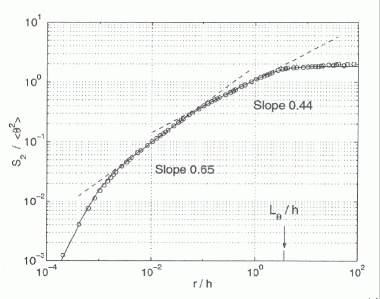
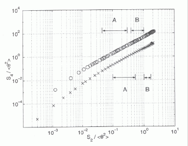
Figure 1: Normal structure function of the temperature fluctuations. Top figure: $S_{2}({\bf r})$ is shown for height $h=1.75$ m above the ground. Shown by the vertical arrow on the abscissa is the integral scale $L_{\theta}$ for the temperature fluctuations. Bottom figure: $S_{4}({\bf r})$ as a function of $S_{2}({\bf r})$. The data corresponding to the top figure are marked as circles (multiplied, for convenience, by a factor of 10). A and B, which have the same slope in the bottom figure, correspond to the two scaling ranges with slopes of 0.65 and 0.44, respectively, in the top figure. The crosses in the bottom figure correspond to another similar situation where A and B, again, have two distinctly different slopes for normal structure functions. Both figures are reproduced from Ref. kga_krs_01 .

The second comment is that the structure functions, Eqs. (1) and (2), have different sign-symmetry properties. One has to distinguish the sign-symmetry with respect to the reversal of increments $\Delta_{\bf r}\to-\Delta_{\bf r}$ from that with respect to spatial reflection (also known as parity)—that is, for the transformation ${\bf r}\to-{\bf r}$. The absolute structure functions (2) remain unchanged for all orders $n$ under both transformations; they have even sign-symmetry. The same is true for even-order normal structure functions but the odd-order normal structure functions change sign under both transformations; they have odd sign-symmetry or sign-antisymmetry. Note that $\Delta_{\bf r}\to-\Delta_{\bf r}$ does not follow from ${\bf r}\to-{\bf r}$ although, for homogeneous turbulence, both transformations have the same effect on (1). We wish to comment on ESS in the light of the sign-symmetry properties of structure functions. For this purpose, it is convenient to introduce new types of structure functions which explicitly emphasize the sign-symmetry with respect to the increment $\Delta_{\bf r}$. This is our basic goal.

These new quantities, along with (1) and (2), will be calculated from temperature data from a high-Reynolds-number atmospheric boundary layer. The Taylor microscale Reynolds number is about 3500. Since the experiments have been described in some detail in Kurien1 , we shall mention only a few details here. Measurements were made in a boundary layer above salt flats of the Dugway Proving Ground in Utah, at a height of 1.75 m above the ground. The ground was smooth on the order of a millimeter. Taylor hypothesis was used and $u_{rms}/\overline{U}$ was about 7% with the mean speed $\overline{U}=0.72$ ms^-1. Measurements were made at various times of the day, covering intensely convective motion in late afternoon, essentially neutral conditions in the evening hours and somewhat stable conditions until about 11 PM. The data records chosen for analysis corresponded to constant wind conditions in magnitude as well as direction. Temperature fluctuations were measured by two cold wires of 0.6 $\mu$m diameter and 1 mm length. The data acquisition system was a standard constant-current anemometer system operated at a small enough current to minimize velocity sensitivity.

The paper is organized as follows. In Sec. II, we will construct the new types of structure functions, in line with the approach of Sreeni96 for velocity increments. Since these structure functions are of intrinsic interest, they are presented first before considering ESS. Section III contains the results of the ESS data analysis for structure functions with even and odd sign-symmetry. In Sec. IV, we discuss a possible explanation of the effects observed in terms of the SO(3) rotation group decomposition of structure functions of different sign-symmetry. Some concluding remarks are presented in Sec. V.

II Sign-symmetry with respect to the temperature increment

Let the probability density function (PDF) of the temperature increment at fixed distance vector ${\bf r}$ be given by $f(\Delta_{\bf r})$. First, we can define (1) and (2) as

$$S_{n} = \int_{-\infty}^{\infty}\Delta_{\bf r}^{n}f(\Delta_{\bf r})d\Delta_{\bf r}$$ (3)

$$S_{|n|} = \int_{-\infty}^{\infty}{|\Delta_{\bf r}|}^{n}f(\Delta_{\bf r})d\Delta_{\bf r}\,.$$ (4)

The PDF can be decomposed into its symmetric and antisymmetric parts with respect to the increment as

$$f_{s}(\Delta_{\bf r}) = \frac{f(\Delta_{\bf r})+f(-\Delta_{\bf r})}{2}$$ (5)

$$f_{a}(\Delta_{\bf r}) = \frac{f(\Delta_{\bf r})-f(-\Delta_{\bf r})}{2}\,.$$ (6)

Note that $f_{a}$ does not have the positive-definite property of a PDF.

We can also define the positive and negative parts of the PDF as

$$p(\Delta_{\bf r},\Delta_{\bf r}\geq 0) = f(\Delta_{\bf r})$$ (7)

$$n(\Delta_{\bf r},\Delta_{\bf r}\geq 0) = f(-\Delta_{\bf r}),\$$ (8)

and define moments of $\Delta_{\bf r}$ with respect to $f_{s}$, $f_{a}$, $p$ and $n$, respectively, by the following relations:

$$P_{n} = \int_{0}^{\infty}\Delta_{\bf r}^{n}~{}p(\Delta_{\bf r})d\Delta_{\bf r},$$ (9)

$$N_{n} = \int_{0}^{\infty}\Delta_{\bf r}^{n}~{}n(\Delta_{\bf r})d\Delta_{\bf r},$$ (10)

$$S_{n,s} = 2\int_{0}^{\infty}\Delta_{\bf r}^{n}~{}f_{s}(\Delta_{\bf r})d\Delta_{\bf r},$$ (11)

$$S_{n,a} = 2\int_{0}^{\infty}\Delta_{\bf r}^{n}~{}f_{a}(\Delta_{\bf r})d\Delta_{\bf r}\,.$$ (12)

The following relations are now valid:

$$S_{n,s} = P_{n}+N_{n}=S_{|n|}$$ (13)

$$S_{n,a} = P_{n}-N_{n}\,.$$ (14)

For odd values of $n=2k+1$, Eq. (14) reduces to the normal odd-order structure function

$$S_{2k+1,a}=P_{2k+1}-N_{2k+1}=S_{2k+1}\,,$$ (15)

whereas, for even $n=2k$, Eq. (14) is a new structure function which is $even$ order, but sign-$antisymmetric$. It is not possible to have this combination in terms of either normal or absolute structure functions.

On the basis of the discussion of the sign-symmetries of $f_{s}$ and $f_{a}$, using the definitions (7) and (8), it is clear that

$$P_{n}+N_{n} = \int_{0}^{\infty}\Delta_{\bf r}^{n}(p(\Delta_{\bf r})+n(\Delta_{\bf r}))d\Delta_{\bf r}$$ (16)

$$= \int_{0}^{\infty}\Delta_{\bf r}^{n}(f(\Delta_{\bf r})+f(-\Delta_{\bf r}))d\Delta_{\bf r}$$

is sign-symmetric, while

$$P_{n}-N_{n} = \int_{0}^{\infty}\Delta_{\bf r}^{n}(p(\Delta_{\bf r})-n(\Delta_{\bf r}))d\Delta_{\bf r}$$ (17)

$$= \int_{0}^{\infty}\Delta_{\bf r}^{n}(f(\Delta_{\bf r})-f(-\Delta_{\bf r}))d\Delta_{\bf r}$$

is sign-antisymmetric.

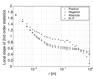
(a) Logarithmic local slopes of the various structure functions for $n=2$

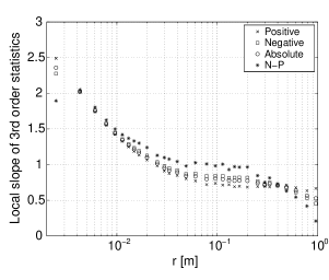
(b) Logarithmic local slopes of the various structure functions for $n=3$.

Figure 2: Local slopes in the log-log graphs of four types of structure functions: positive ($P_{n}$) and negative ($N_{n}$) parts, the sum of positive and negative parts (same as the absolute moment), $S_{|n|}=P_{n}+N_{n}=S_{n,s}$, and the negative minus the positive part, $|S_{n}|=N_{n}-P_{n}=|S_{n,a}|$.

To illustrate the differences between normal and absolute structure functions, we plot in Fig. 2 the logarithmic local slopes for four types of moments: $P_{n}$, $N_{n}$, $S_{n,s}$ and $S_{n,a}$. Figure 2(a) show these quantities for $n=2$. Here $S_{2,a}$ is the normal (and absolute) second order structure function; $|S_{2,a}|=N_{2}-P_{2}$ is the newly defined sign-antisymmetric second order structure function. Figure 2(b) shows the same four quantities for $n=3$. Although the scaling is not impeccable even at this high Reynolds number (see Ref. Sreeni98 for comments in this regard on the scaling of velocity structure functions), a scaling tendency can be discerned in the range between a few mm and a few cm.

Independent of this detail, it is clear that the exponents, if one were to assign nominal values in the scaling range, are not the same for all the different structure functions of the same order. In particular, the second-order sign-antisymmetric structure function $|S_{2,a}|=N_{2}-P_{2}$ has a substantially larger exponent than the classical exponent of 2/3. While $S_{3,a}=S_{3}$ has a scaling exponent close to the Kolmogorov prediction of 1, the other curves have measurably smaller scaling exponents. In particular, the absolute structure functions have smaller scaling exponents than the normal structure function.

At the least, these features are disconcerting to anyone interested in scaling exponents. An understanding of differences in the exponents of the various types of structure functions may help in this regard. This will be attempted in the next section.

III Analysis using Extended Self-Similarity

(a) Loglog plot of $S_{2}$ vs. $S_{|3|}$

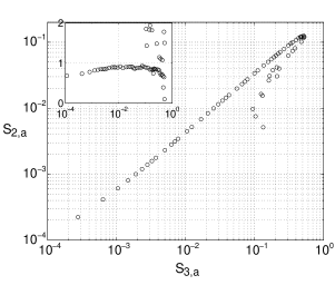
(b) Loglog plot of $S_{2,a}$ vs. $S_{3,a}$

Figure 3: ESS comparisons of structure functions of different order and same sign-symmetry. Insets show the (logarithmic) local slope in these ESS coordinates. In this comparison, only one scaling exponent is seen past the dissipation range. The conditions for this and other figures to follow are the same as for Fig. 1.

In this section, we shall examine ESS of scalar statistics in the light of the new objects defined in terms of their parity. We first apply ESS as is normally done for velocity statistics: plot structure functions of all orders against the absolute third-order structure function. We shall follow this practice for illustrative purposes, even though the third-order does not have a comparably significant meaning for temperature. In Fig. 3(a), the ESS plot of $S_{2}(r)$ versus $S_{|3|}$ shows a single relative scaling exponent outside the dissipative range. The inset shows the local logarithmic slope of the extended self-similarity plot which is calculated via $D_{2,|3|}=\mbox{d}\log(S_{2}(r))/\mbox{d}\log(S_{|3|}(r))$. However, this same signal has two scaling regions with distinct exponents when plotted against $r$ (corresponding to the passive range at small scales and the convective range at large scales, see top panel of Fig. 1). This two-exponent scaling behavior is masked by ESS. This is essentially so even if we plot the sign-antisymmetric structure function of the second-order against $S_{3}$ (which is also sign-antisymmetric, see Sec. 2), as seen in Fig. 3(b).

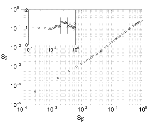
(a) Loglog plot of $S_{3}$ vs. $S_{|3|}$

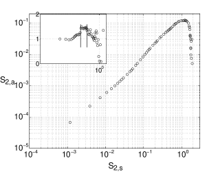
(b) Loglog plot of $S_{2,a}$ vs. $S_{2,s}$

Figure 4: ESS comparisons of structure functions of the same order and different sign-symmetry. Inset shows the (logarithmic) local slope in these ESS coordinates. For this comparison, the two different scaling regimes are retreived. Vertical bars are inserted in order to show regions of constant local slope.

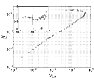
(a) Loglog plot of $S_{2,s}$ vs. $S_{3,a}$

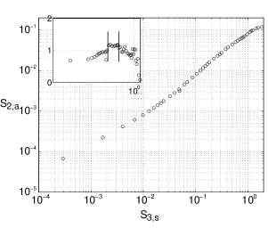
(b) Loglog plot of $S_{2,a}$ vs. $S_{3,s}$

Figure 5: ESS comparisons of structure functions of different order and different sign-symmetry. The insets show the (logarithmic) local slope in these ESS coordinates. Once again, two different scaling regimes are retrieved. Vertical bars are inserted in order to show regions of constant local slope.

Let us now compare objects of the same order, but different sign-symmetry. In Fig. 4(a), we show a plot of $S_{3}(r)$ which is odd-parity (made of the antisymmetric combination of the PDF functions) versus $S_{|3|}(r)$, which is the corresponding even-parity object of the same order. The two objects scale identically in the smallest (dissipative/diffusive) scales with relative exponent of unity, transitioning into a region of relative exponent 1.27. This corresponds to the inertial range scaling, as we already know from Fig. 2. Past this range, the relative scaling exponent drops back to $\sim 1$. In Fig. 4(b), we repeat the ESS comparison for the second-order. Instead of plotting the second-order object against another order, we choose to compare the even- and odd-parity manifestations $S_{2,s}(r)=S_{2}(r)$ and $S_{2,a}(r)$, respectively. Once again, it is seen that there are two regions of scaling beyond the dissipative range. The small-scale range has a relative scaling exponent of about 1 while the large-scale range has a slope of 1.42. These exponents are as expected from the direct scaling analysis of kga_krs_01 .

Finally, when we compare objects of different order $and$ different parity as shown in Fig. 5, the dual scaling range feature persists. Figure 5(a) shows $S_{2,s}=S_{2}(r)$ versus $S_{3,a}=S_{3}(r)$ while Fig. 5(b) shows $S_{2,a}$ vs. $S_{3,s}=S_{|3|}(r)$. Again, we recover two separate scaling ranges, one inertial and one convective.

From these examples, we can now make the following general statement. In a process with two distinct scaling ranges, ESS cannot distinguish between them whenever a comparison is made between two like-parity objects. However, if ESS compares objects of $any$ order, but of opposite parity, a second scaling (if it exists) can be recovered. This is our major qualitative conclusion. This kind of comparison has been made possible by the introduction of the odd-symmetry, even-order objects $S_{n,a}(r)$ ($n$ even)—which, to our knowledge, have not been considered before.

IV Parity of the new moments from the viewpoint of SO(3) decomposition

We shall now discuss the above property of ESS from another perspective that contains the correct description of the parity property. We consider an analytical expression for structure functions with two distinct scaling ranges, separated by a crossover scale $l_{c}$. Since we do not know the proper analytical expression for the structure functions, we use an empirical interpolation formula. Batchelor’s attempt Batchelor51 in this direction has been extended variously, in particular in Refs. stolo_sreeni1 ; stolo_sreeni2 , for structure functions of all orders. Here, we shall extend the specific form proposed in Ref. Fujisaka01 to the $n$th order as

$$S_{n}(r)\sim\left(\frac{r}{l_{c}}\right)^{\alpha_{n}}\,\left[g\left(\frac{r}{l_{c}}\right)\right]^{\alpha_{n}-\beta_{n}}\,,$$ (18)

with the function

$$g(x)=\frac{1}{(1+x^{\kappa})^{1/\kappa}}\,,$$ (19)

where the assumed scaling exponents $\alpha_{n}$ hold for the passive range, $r\ll l_{c}$, and $\beta_{n}$ for the convective range, $r\gg l_{c}$, and $\alpha_{n}>\beta_{n}$; $g(x)$ is a dimensionless function that is monotonically decreasing, and the exponent $\kappa>1$ determines the width of the crossover from one scaling range to the other.

We make use of the $spatial$ $parity$ of the signed structure functions by noting that, in homogeneous turbulence, $S_{n,s}({\bf r})=S_{|n|}({\bf r})$ is even-parity with respect to reflection under ${\bf r}\rightarrow-{\bf r}$ for all $n$; the odd-order normal structure functions $S_{2k+1,a}({\bf r})=S_{2k+1}({\bf r})$ are odd-parity; the newly defined $S_{2k,a}$, even-order sign-$antisymmetric$ statistics are odd-parity as well. So, in the homogeneous case the sign-symmetry with respect to the increment is the $same$ as the sign-symmetry with respect to the spatial orientation of ${\bf r}$ (i.e. parity) and this allows for the following decomposition of the objects defined in Sec. II.

The recently developed SO(3) group decomposition Arad99 applies conveniently to the symmetric and antisymmetric structure functions. For the scalar case, the basis functions are spherical harmonics $Y_{l,m}({\bf\hat{r}})$ Kurien2 . The even or odd spatial parity is carried by the angular dependence in the spherical harmonics, in effect by the index $l$, as

$$Y_{l,m}(-\hat{\bf r})=(-1)^{l}Y_{l,m}(\hat{\bf r})$$ (20)

Perfectly isotropic objects would contain an $l=0$ sector only, i.e., no angular dependence would be present. Sign-symmetric functions are composed of only even sectors while sign-antisymmetric functions are composed only of odd sectors. Thus,

$$S_{n,s}(r,\theta,\phi) =S_{n,s}^{(0)}(r)+S_{n,s}^{(2)}(r,\theta,\phi)+\dots,$$

$$= \sum_{k=0}^{\infty}\sum_{m=-2k}^{2k}A_{2k,m}r^{\zeta_{n}^{(2k)}}Y_{2k,m}(\theta,\phi),$$

where the superscripts $(0)$, $(2)$, $\dots$ denote the even-parity contributions allowed, and

$$S_{n,a}(r,\theta,\phi) =S_{n,a}^{(1)}(r,\theta,\phi)+S_{n,a}^{(3)}(r,\theta,\phi)+\dots,$$

$$= \sum_{k=0}^{\infty}\sum_{m=-2k-1}^{2k+1}A_{2k+1,m}r^{\zeta_{n}^{(2k+1)}}Y_{2k+1,m}(\theta,\phi),$$

where the superscripts $(1)$, $(3)$, $\dots$ denote the odd-parity contributions allowed. We can substitute the algebraic scaling form of (18) for each scaling term in (IV) and (IV) to obtain

$$S_{n,s}(r,\theta,\phi)=\sum_{k,m} A_{2k,m}\left(\frac{r}{l_{c}}\right)^{\alpha_{n}^{(2k)}}$$ (23)

$$\times \left[g\left(\frac{r}{l_{c}}\right)\right]^{\alpha_{n}^{(2k)}-\beta_{n}^{(2k)}}$$

$$\times Y_{2k,m}(\theta,\phi)\,,$$

and

$$S_{n,a}(r,\theta,\phi)=\sum_{k,m} A_{2k+1,m}\left(\frac{r}{l_{c}}\right)^{\alpha_{n}^{(2k+1)}}$$ (24)

$$\times \left[g\left(\frac{r}{l_{c}}\right)\right]^{\alpha_{n}^{(2k+1)}-\beta_{n}^{(2k+1)}}$$

$$\times Y_{2k+1,m}(\theta,\phi)\,.$$

The finding that ESS yields the same relative exponents, when comparisons are made of even-parity statistics, means that for all sectors and for any pair of orders $(p,q)$ we have

$$\frac{\alpha_{p}^{(2k)}}{\alpha_{q}^{(2k)}}=\frac{\beta_{p}^{(2k)}}{\beta_{q}^{(2k)}}\,.$$ (25)

Equivalently, for $p<q$, it follows that

$$\frac{\alpha_{p}^{(2k)}}{\alpha_{p}^{(2k)}\,\Pi_{i=p}^{q-1}\left(1+\delta_{i}^{(2k)}\right)}=\frac{\beta_{p}^{(2k)}}{\beta_{p}^{(2k)}\,\Pi_{i=p}^{q-1}\left(1+\delta_{i}^{(2k)}\right)}\,,$$ (26)

where the quantities

$$\delta_{p}^{(2k)}=\frac{\alpha_{p+1}^{(2k)}-\alpha_{p}^{(2k)}}{\alpha_{p}^{(2k)}}\,,$$ (27)

are the relative increments between successive orders. The constraint (25) means that the relative increments in both convex functions, $\alpha_{p}(p)$ as well as $\beta_{p}(p)$, are equal. This was already shown in Ref. Benzi96 , where physically different turbulent states such as the Kolmogorov turbulence in three dimensions, thermal convection as well as magnetohydrodynamic turbulence showed the same relative ESS exponents. We suppose, therefore, that as long as the different regimes belong to the same “universality class”—i.e., if they have the same relative increments $\delta_{n}^{(2k)}$ for all orders $n$—ESS will simply mask the presence of distinct scaling regimes.

The argument for the odd-parity ESS comparisons is similar, now with the constraint

$$\frac{\alpha_{p}^{(2k+1)}}{\alpha_{q}^{(2k+1)}}=\frac{\beta_{p}^{(2k+1)}}{\beta_{q}^{(2k+1)}}\,.$$ (28)

One remains within a universality class when plotting $S_{p,a}(r)$ as functions of $S_{q,a}(r)$, but it can be expected that the relative exponents will be different from those for the even parity case.

We now turn to the case where $S_{p,s}(r)$ are compared to $S_{q,a}(r)$, which are objects with different symmetries. When proceeding as in (25), (26), and (27) we obtain

$$\frac{\alpha_{p}^{(2k)}}{\alpha_{p}^{(2k+1)}\Pi_{i=p}^{q-1}\left(1+\epsilon_{i}^{(2k+1)}\right)}=\frac{\beta_{p}^{(2k)}}{\beta_{p}^{(2k+1)}\Pi_{i=p}^{q-1}\left(1+\epsilon_{i}^{(2k+1)}\right)}.$$

For insensitivity to different scaling regimes, the following must hold true:

$$\frac{\alpha_{p}^{(2k)}}{\alpha_{p}^{(2k+1)}}=\frac{\beta_{p}^{(2k)}}{\beta_{p}^{(2k+1)}}\,.$$ (29)

Recall that the superscript $(2k)$ corresponds to even parity objects while $(2k+1)$ corresponds to odd parity. We expect that several mechanisms, such as the breaking of reflection symmetry by a mean gradient for scales $r<l_{c}$ or by buoyancy effects for scales $r>l_{c}$, will lead to different ratios on the left and right hand side of the Eq. (29), respectively, thus leading to a “discontinuity” in scaling. While this discussion cannot be a proof of our main observation, it shows that the two scaling regimes belong to different universality classes when different parities are involved. Further, it provides hints for what kind of quantities have to be investigated in order to shed more light on the issue, in experiments as well as in numerical simulations.

V Conclusions

We have analyzed moments of temperature increments with respect to their sign-symmetry properties, and defined sign-symmetric and sign-antisymmetric components for both even and odd-order structure functions. ESS analysis of all combinations of symmetry and order of structure functions indicates that this technique masks the convective scaling regime. Only if objects of opposite parity are compared can one recover the distinct scalings.

We have presented a model for how such scaling regimes behave in the ESS analysis using even and odd orders of a spherical harmonic expansion. Unfortunately, this model cannot be taken to its logical conclusion because the various numerical coefficients cannot be obtained with any certainty from the existing data. Furthermore, a dependence on the strength of the mean temperature gradient might modify some of our results as well—e.g., differences in the exponents of even order moments in comparison to odd order moments.

One purpose here has been to point out the possible pitfalls in using ESS without proper consideration of the symmetry properties of the statistics being compared. This observation does not detract from the merits of the method. Indeed, ESS has proved to be a very useful tool in extracting exponents when the scaling range with respect to $r$ is short.

- (1) A. M. Obukhov, Isv. Geogr. Geophys. Ser. 13, 58 (1949).
- (2) S. Corrsin, J. Appl. Phys. 22, 469 (1951).
- (3) A. S. Monin and A. M. Yaglom, Statistical Fluid Mechanics. MIT Press, Cambridge, MA, 1975.
- (4) R. A. Antonia, Hopfinger, E., Gagne, Y. and F. Anselmet, Phys. Rev. A 30, 2704 (1984).
- (5) F. Moisy, H. Willaime, J. S. Andersen and P. Tabeling, Phys. Rev. Lett. 86, 4827 (1999).
- (6) R. Benzi, L. Biferale, S. Ciliberto, M. V. Struglia and R. Tripiccione, Physica D 96, 162 (1996).
- (7) K. G. Aivalis, K. R. Sreenivasan, Y. Tsuji, J. C. Klewicki, and C. A. Biltoft, Phys. Fluids 14, 2439 (2002).
- (8) S. Kurien, K. G. Aivalis, and K. R. Sreenivasan, J. Fluid Mech. 448, 279 (2001).
- (9) K. R. Sreenivasan, S. I. Vainshtein, R. Bhiladvala, I. San Gil, S. Chen, and N. Cao, Phys. Rev. Lett. 77, 1488 (1996).
- (10) K. R. Sreenivasan and B. Dhruva, Prog. Theo. Phys. 130, 103 (1998).
- (11) G. K. Batchelor, Proc. Camb. Philos. Soc. 47, 359 (1951).
- (12) G. Stolovitzky and K. R. Sreenivasan, Phys. Rev. E 48, R33 (1993).
- (13) G. Stolovitzky, K. R. Sreenivasan, and A. Juneja, Phys. Rev. E 48, R3217 (1993).
- (14) H. Fujisaka and S. Grossmann, Phys. Rev. E 63, 026305 (8 pages) (2001).
- (15) I. Arad, V. S. L’vov, and I. Procaccia, Phys. Rev. E 59, 6753 (1999).
- (16) S. Kurien and K. R. Sreenivasan, Measures of anisotropy and the universal properties of turbulence. In Les Houches Summer School Proceedings 2000, pp. 53-111, Springer-EDP (2001).