Integrable equations in nonlinear geometrical optics.

Abstract

Geometrical optics limit of the Maxwell equations for nonlinear media with the Cole-Cole dependence of dielectric function and magnetic permeability on the frequency is considered. It is shown that for media with slow variation along one axis such a limit gives rise to the dispersionless Veselov-Novikov equation for the refractive index. It is demonstrated that the Veselov-Novikov hierarchy is amenable to the quasiclassical $\bar{\partial}$-dressing method. Under more specific requirements for the media, one gets the dispersionless Kadomtsev-Petviashvili equation. Geometrical optics interpretation of some solutions of the above equations is discussed.

PACS numbers: 02.30.Ik, 42.15.Dp
Key words: Nonlinear Optics, Integrable Systems.

1 Introduction.

Nonlinear optics provides us with various, very interesting nonlinear phenomena (see e.g. [1, 2]). At the same time, it is the source of several nonlinear differential equations, modelling such phenomena, with certain very special properties. The nonlinear Schrödinger (NLS) equation, which describes self-modulation and self-focusing of electromagnetic waves in nonlinear media [1, 2] is, perhaps, the most known one. The NLS equation is integrable by the inverse scattering transform method and has a number of remarkable properties (multisoliton solutions, infinite set of conserved quantities and so on). Nowadays there are a number of the, so-called, integrable nonlinear differential equations which have similar properties [3, 4]. A subclass of such equations, referred usually as dispersionless integrable equations, has attracted a particular interest in the last years (see e.g. [5]-[11]).

In the present paper we will study integrable structures which arise within the geometrical optics of nonlinear media. We will consider nonlinear media which are characterized by the Cole-Cole dependence of dielectric function and magnetic permeability on the frequency and slow variation of all quantities along one axis. We will show that the propagation of monochromatic electromagnetic waves of high frequency $\omega$ in such media is governed by the dispersionless Veselov-Novikov (dVN) equation. Namely, we will demonstrate that the Maxwell equation in such a situation in the limit $\omega\rightarrow\infty$ gives rise to the standard plane eikonal equation accompanied by the equation which describes its deformation in the orthogonal direction. The compatibility of these two equations is equivalent to dVN equation for the refractive index. This dVN deformations of the plane eikonal equation preserve, in particular, the total “plane” squared refractive index $\int\int n^{2}dxdy$. We will show also that under more specific conditions, the Maxwell equation is reduced to the dispersionless Kadomtsev-Petviashvili (dKP) equation.

In this paper, we will demonstrate that the plane eikonal equation as well as the dVN equation and whole dVN hierarchy, both for complex and real-valued refractive indices are treatable by the quasiclassical $\bar{\partial}$-dressing method recently developed in [12, 13, 14]. The characterization conditions for the $\bar{\partial}$-data, symmetry constraints for the dVN equation and associated hodograph type solutions are also studied. Geometrical optics interpretation of some solutions of dKP and dVN equations is discussed too.

The paper is organized as follows. In section 2 we discuss general properties of nonlinear media under consideration. In section 3 the dVN equation is derived as the geometrical optics limit of the Maxwell equations. The particular case of the dKP equation is discussed in section 4. The quasiclassical $\bar{\partial}$-dressing method is applied to the plane eikonal equation in the section 5. The dVN equation is treated in the next section 6. Characterization conditions for $\bar{\partial}$-data are considered in section 7. Symmetry constraints for dVN equation and associated hodograph type solutions are discussed in section 8. At the last section 9 we present several exact and numerical solutions both for dVN and dKP equations and corresponding wavefronts.

Some results of this paper have been announced in the letter [15].

2 Maxwell equations in nonlinear media.

We begin with the Maxwell equations in the absence of sources (we put the velocity of the light in the vacuum $c=1$)

$$\nabla\wedge{\mathbf{H}}-{\mathbf{\dot{}}{D}}=0~{}~{}~{}~{}~{}~{}\nabla\cdot{\mathbf{D}}=0$$

$$\nabla\wedge{\mathbf{E}}+{\mathbf{\dot{}}{B}}=0~{}~{}~{}~{}~{}~{}~{}\nabla\cdot{\mathbf{B}}=0$$ (2.1)

and the material equations of a medium

$${\mathbf{D}}=\varepsilon{\mathbf{E}},~{}~{}~{}~{}~{}~{}{\mathbf{B}}=\mu{\mathbf{H}}.$$ (2.2)

Here and below $\nabla=\left(\partial_{x},\partial_{y},\partial_{z}\right)$, while $\cdot$ and $\wedge$ denote the scalar and vector product respectively.

We will study a propagation of electromagnetic waves of the fixed, high frequency $\omega$, i.e. we will look for the solutions of the Maxwell equations of the form [16]

$${\mathbf{E}}\left(x,y,z,t\right)={\mathbf{E}_{0}}\left(x,y,z\right)e^{-i\omega t}={\mathbf{\tilde{}}{E}_{0}}\left(x,y,z\right)e^{-i\omega t+i\omega S\left(x,y,z\right)}$$

$${\mathbf{H}}\left(x,y,z,t\right)={\mathbf{H}_{0}}\left(x,y,z\right)e^{-i\omega t}={\mathbf{\tilde{}}{H}_{0}}\left(x,y,z\right)e^{-i\omega t+i\omega S\left(x,y,z\right)}$$ (2.3)

where ${\mathbf{E}_{0}}$, ${\mathbf{H}_{0}}$ and the phase $S\left(x,y,z\right)$ are certain functions and ${\mathbf{\tilde{}}{E}_{0}}=\sum_{n=0}^{\infty}\omega^{-n}{\mathbf{E}_{0}}_{,n}(x,y,z)$, ${\mathbf{\tilde{}}{H}_{0}}=\sum_{n=0}^{\infty}\omega^{-n}{\mathbf{H}_{0}}_{,n}(x,y,z)$.

Maxwell equations (2-2.2) imply the following stationary second order equations for ${\mathbf{E}_{0}}$ and ${\mathbf{H}_{0}}$ [16]

$$\nabla^{2}{\mathbf{E}_{0}}+\omega^{2}\mu\varepsilon{\mathbf{E}_{0}}+\left(\nabla\log~{}\mu\right)\wedge\left(\nabla\wedge{\mathbf{E}_{0}}\right)+\nabla\left({\mathbf{E}_{0}}\cdot\nabla\log~{}\varepsilon\right) = 0$$

$$\nabla^{2}{\mathbf{H}_{0}}+\omega^{2}\mu\varepsilon{\mathbf{H}_{0}}+\left(\nabla\log~{}\varepsilon\right)\wedge\left(\nabla\wedge{\mathbf{H}_{0}}\right)+\nabla\left({\mathbf{H}_{0}}\cdot\nabla\log~{}\mu\right) = 0.$$ (2.4)

We assume that the medium is characterized by the Cole-Cole dependence [17] of the dielectric function $\varepsilon$ and the magnetic permeability $\mu$, namely, that

$$\varepsilon=\varepsilon_{0}+\frac{\tilde{\varepsilon}}{1+\left(i\omega\tau_{0}\right)^{2\nu}},~{}~{}~{}~{}~{}~{}0<\nu<\frac{1}{2}$$ (2.5)

and

$$\mu=\mu_{0}+\frac{\tilde{\mu}}{1+\left(i\omega\tau_{0}\right)^{2\nu}},~{}~{}~{}~{}~{}~{}0<\nu<\frac{1}{2}$$ (2.6)

where $\varepsilon_{0}$, $\mu_{0}$ depend on the coordinates $x,y,z$, while $\tilde{\varepsilon}$ and $\tilde{\mu}$ depend both on the coordinates and the moduli of the fields and their derivatives. In the high frequency limit $\omega\rightarrow\infty$ we have

$$\varepsilon=\varepsilon_{0}(x,y,z)+\frac{\tilde{\varepsilon_{1}}}{\omega^{2\nu}}$$

$$\mu=\mu_{0}(x,y,z)+\frac{\tilde{\mu_{1}}}{\omega^{2\nu}}$$ (2.7)

where $\tilde{\varepsilon_{1}}=(i\tau_{0})^{-2\nu}\tilde{\varepsilon}$ and $\tilde{\mu_{1}}=(i\tau_{0})^{-2\nu}\tilde{\mu}$. In some textbooks (see e.g. [18, 19]) it is argued that at $\omega\rightarrow\infty$ the dielectric function has the following asymptotic behaviour

$$\varepsilon(\omega)\rightarrow 1+\frac{{const}}{\omega^{2}},~{}~{}~{}~{}\omega\rightarrow\infty.$$ (2.8)

Experimental results of the Cole and Cole [17] have demonstrated that the theoretical models behind the formula (2.8) are not always correct. The fact that the parameter $\nu$ in the Cole-Cole dependence (2.5) and (2.6) belongs to the interval $\left(0,\frac{1}{2}\right)$ is of crucial importance for our study.

At limit $\omega\rightarrow\infty$, $\varepsilon$ and $\mu$ may depend on the derivatives $S_{x},S_{y},S_{z}$. Different mechanism may be responsible for such a dependence. One is provided by a non-local spatial dependence of ${\mathbf{D}}$ on ${\mathbf{E}}$. Indeed, let us assume that a monochromatic wave of frequency $\omega$ of the form (2) propagating in a medium have a spatial non-local dependence for the displacement $\mathbf{D}({\mathbf{x}},t)$ on $\mathbf{E}({\mathbf{x}},t)$ of the standard form

$${\mathbf{D}_{0}}({\mathbf{x}},\omega)=\int\int\int_{\mathbb{R}^{3}}g({\mathbf{x}^{\prime}-x},\omega){\mathbf{E}_{0}}({\mathbf{x}^{\prime}-x},\omega)d{\mathbf{x}^{\prime}}.$$ (2.9)

In the particular case where the distribution $g({\mathbf{x}},\omega)$ is proportional to a $\delta$-Dirac function

$$g({\mathbf{x}},\omega)=\varepsilon({\mathbf{x}},\omega)\delta({\mathbf{x}^{\prime}-x})$$ (2.10)

one obtains the usual material equation (2.2). Here, we consider non-local effects involving a linear superposition of derivatives $\delta$-functions in the following way

$$g({\mathbf{x}},\omega)=\sum_{l,m,n=0}^{\infty}g_{l,m,n}({\mathbf{x}},\omega)\delta^{(l,m,n)}({\mathbf{x}^{\prime}-x}).$$ (2.11)

The distributions $\delta^{(l,m,n)}$ are defined standardly as

$$\int\int\int_{\mathbb{R}^{3}}f({\mathbf{x}^{\prime}})\delta^{(l,m,n)}({\mathbf{x}^{\prime}-x})d{\mathbf{x}^{\prime}}=(-1)^{l+m+n}\frac{\partial^{l+m+n}f({\mathbf{x}})}{\partial x_{1}^{l}\partial x_{2}^{m}\partial x_{3}^{n}},$$ (2.12)

for a function $f({\mathbf{x}})$ defined in $\mathbb{R}^{3}$ and ${\mathbf{x}}=(x_{1},x_{2},x_{3})$. With the use of the (2.11) the formula (2.9) for the $jth$ component of the field, for $j=1,2,3$ can be written as

$$D_{0j}({\mathbf{x}},\omega)=\varepsilon_{j}E_{0j}({\mathbf{x}},\omega)$$ (2.13)

where the factors $\varepsilon_{j}$ are given by

$$\varepsilon_{j}({\mathbf{x}},\omega)=\sum_{l,m,n=0}^{\infty}(-1)^{l+m+n}\frac{g_{l,m,n}({\mathbf{x}},\omega)}{E_{0j}({\mathbf{x}},\omega)}\frac{\partial^{l+m+n}E_{0j}({\mathbf{x}},\omega)}{\partial x_{1}^{l}\partial x_{2}^{m}\partial x_{3}^{n}}.$$ (2.14)

Assuming that in the limit $\omega\rightarrow\infty$ $g_{000}$ does not depend on the frequency, while

$$g_{l,m,n}({\mathbf{x}},\omega)\longrightarrow\frac{1}{\omega^{2\nu+l+m+n}}\tilde{g}_{l,m,n}({\mathbf{x}});~{}~{}~{}~{}~{}~{}\omega\rightarrow\infty,$$ (2.15)

one gets the formula (2) from (2.14), where $\tilde{\varepsilon}$ and $\tilde{\mu}$ depend on $S_{x}$, $S_{y}$ and $S_{z}$.

We note that a number of dielectrics has the Cole-Cole dependence of dielectric function $\varepsilon$ on $\omega$ [17, 20, 21], while for most of studied media the magnetic permeability $\mu$ does not depend on $\omega$. In this paper, however, for the sake of completeness we will consider the general case (2). Note also that at $\omega\rightarrow\infty$ certain typical effects on nonlinearity, like a second-harmonic generation, become irrelevant.

In addition to the Cole-Cole property we assume that the medium is anisotropic one, that is all quantities (${\mathbf{E}}$, ${\mathbf{H}}$, $\varepsilon$, $\mu$) vary slowly along the axis $z$, such that, formally, $f_{z}=\omega^{-\nu}f_{\xi}$, (here and below $f_{z}=\frac{\partial f}{\partial z}$ etc.) and $\xi$ is a “slow” variable defined by $z=\omega^{\nu}\xi$. More precisely, we assume that at $\omega\rightarrow\infty$

$$f(x,y,\omega^{\nu}\xi)=f_{0}(x,y,\xi)+\omega^{-\nu}f_{1}(x,y,\xi)+\omega^{-2\nu}f_{2}(x,y,\xi)+\dots.$$ (2.16)

We would like to note that the Cole-Cole property (2) is quite generic and has been widely discussed, while the particular type of slow variation along the axis $z$ given by (2.16), seems, did not attract attention before.

3 dVN equation as the geometrical optics limit of the Maxwell equations.

Now we will analyze the squared Maxwell equations (2) for the media described in section 2, i.e. for solutions of the form (2), where at $\omega\rightarrow\infty$

$$S(x,y,\omega^{\nu}\xi)=S(x,y,\xi)+\omega^{-\nu}S_{1}(x,y,\xi)+\omega^{-2\nu}S_{2}(x,y,\xi)+\dots,$$ (3.1)

$$\varepsilon(x,y,\omega^{-\nu}\xi)=\varepsilon_{0}(x,y,\xi)+\omega^{-\nu}\varepsilon_{1}(x,y,\xi)+\omega^{-2\nu}\varepsilon_{2}(x,y,\xi)+\dots,$$ (3.2)

$$\mu(x,y,\omega^{-\nu}\xi)=\mu_{0}(x,y,\xi)+\omega^{-\nu}\mu_{1}(x,y,\xi)+\omega^{-2\nu}\mu_{2}(x,y,\xi)+\dots$$ (3.3)

Taking into account these expansions, one gets in the leading $\omega^{2}$ order the plane eikonal equation

$$S_{x}^{2}+S_{y}^{2}=n^{2}$$ (3.4)

where $n^{2}=\varepsilon_{0}\mu_{0}$. One, obviously, obtains this plane eikonal equation if there is no dependence on $z$ at all.

In the next $\omega^{2-\nu}$ and $\omega^{2-2\nu}$ orders, one gets from (2) the following equations

$$2S_{x}S_{1x}+2S_{y}S_{1y}=\varepsilon_{1}\mu_{0}+\varepsilon_{0}\mu_{1}$$ (3.5)

$$S_{\xi}^{2}=-\left(S_{1x}^{2}+S_{1y}^{2}+2S_{x}S_{2x}+2S_{y}S_{2y}\right)+\varepsilon_{0}\mu_{2}+\varepsilon_{1}\mu_{1}+\varepsilon_{2}\mu_{0}.$$ (3.6)

As we noted in the previous section, $\varepsilon$ and $\mu$ depend, in general, on $S_{x}$,$S_{y}$ and $S_{z}$. Having in mind (3.1-3.3), one concludes that in the order $\omega^{2-\nu}$, $\varepsilon_{1}$, $\mu_{1}$ might depend on the coordinates and only on $S_{x}$ and $S_{y}$. So equation (3.5) defines $S_{1}$ in terms of $S_{x}$ and $S_{y}$. The function $S_{2}$ in equation (3.6) is an undetermined function which in turn might depend on $S_{x}$,$S_{y}$ only. Thus, equation (3.6) assumes the form

$$S_{\xi}=\varphi\left(x,y,\xi;S_{x},S_{y}\right)$$ (3.7)

where $\varphi$ is certain function collecting the contributions of $S_{1}$, $S_{2}$ and $\varepsilon_{j}$, $\mu_{j}$, $j=0,1,2$. Let us note that the dependence of the function $\varphi$ on $S$ is not admissible. Indeed, for the solutions of the form (2) the time-translations symmetry $t\rightarrow t+const$ of the Maxwell equations is equivalent to the phase displacement $S\rightarrow S+const$. In order to preserve this symmetry in equation (3.7), $\varphi$ should depend only on derivatives of the phase function $S$.

Introducing the complex variables $z=x+iy$, $\bar{z}=x-iy$, one rewrites equations (3.4) and (3.7) as follows

$$S_{z}S_{\bar{z}}=u(z,\bar{z},\xi)$$ (3.8)

$$S_{\xi}=\varphi\left(z,\bar{z},\xi;S_{z},S_{\bar{z}}\right)$$ (3.9)

where $u=4n^{2}$.
The condition of compatibility of equations (3.4) and (3.7) (or  (3.8), (3.9)) imposes constraints on the possible forms of the function $\varphi$, namely

$$S_{\bar{z}}\varphi_{z}+S_{z}\varphi_{\bar{z}}+u_{z}\varphi^{\prime}+u_{\bar{z}}\varphi^{\prime\prime}=u_{\xi},$$ (3.10)

where

$$\varphi^{\prime}=\frac{\partial\varphi}{\partial S_{z}}\left(z,\bar{z};S_{z},S_{\bar{z}}\right),~{}~{}~{}~{}~{}~{}\varphi^{\prime\prime}=\frac{\partial\varphi}{\partial S_{\bar{z}}}\left(z,\bar{z};S_{z},S_{\bar{z}}\right).$$ (3.11)

Here we restrict ourself by functions $\varphi$ which are polynomial in $S_{z}$, $S_{\bar{z}}$ and compatible with real-valuedness of $S$ and $u$. For the simplest choice $\varphi=\alpha_{0}(z,\bar{z},\xi)$, equation (3.10) obviously gives $\alpha_{0}=const$, i.e. $u_{\xi}=0,S=\alpha_{0}\xi+\tilde{S}(z,\bar{z})$. For the linear function $\varphi=\alpha S_{z}+\bar{\alpha}S_{\bar{z}}+\beta+\bar{\beta}$, one gets $\alpha=\alpha(z)$, $\beta=const$, and

$$u_{\xi}=\left(\alpha u\right)_{z}+\left(\bar{\alpha}u\right)_{\bar{z}}.$$ (3.12)

For the quadratic

$$\varphi=\alpha S_{z}^{2}+\bar{\alpha}S_{\bar{z}}^{2}+\beta S_{z}+\bar{\beta}S_{\bar{z}}+\gamma+\bar{\gamma},$$ (3.13)

equations (3.10) and (3.8) imply $\alpha=0$, $\beta=\beta(z)$ and $\gamma=const$, i.e. one gets the previous linear case (3.12).

The cubic

$$\varphi=\alpha S_{z}^{3}+\bar{\alpha}S_{\bar{z}}^{3}+\beta S_{z}^{2}+\bar{\beta}S_{\bar{z}}^{2}+\gamma S_{z}+\bar{\gamma}S_{\bar{z}}+\delta+\bar{\delta}$$ (3.14)

obeys equations (3.10) and (3.8) if

$$\alpha=\alpha(z),~{}~{}~{}~{}~{}~{}\beta=0,$$

$$\gamma_{\bar{z}}=-\alpha_{z}u-3\alpha u_{z},$$

$$\delta=const,$$ (3.15)

and one has the equation

$$u_{\xi}=\left(\gamma u\right)_{z}+\left(\bar{\gamma}u\right)_{\bar{z}}.$$ (3.16)

In the particular case $\alpha=1$ and, consequently $\gamma_{\bar{z}}=-3u_{z}$, equation (3.16) is nothing but the dispersionless Veselov-Novikov (dVN) equation introduced in [6, 14].

In a similar manner one can construct higher order nonlinear deformations of wavefronts along $\xi$-direction which correspond to higher degree polynomials $\varphi$. These higher degree cases apparently become physically relevant for the phenomena with large values of $S_{x}$ and $S_{y}$. Thus, if we formally admit all possible degrees of $S_{z}$ and $S_{\bar{z}}$ in the right hand side of equation (3.9), then one has an infinite family of nonlinear equations, which may govern the $\xi$-variations of the wavefronts and “refractive index” $u$. Since equation (3.9) should respects the symmetry $S\rightarrow-S$ of the eikonal equation (3.8), one readily concludes that only polynomials $\varphi$ of the form $\sum_{m=1}^{n}u_{m}S_{z}^{2m-1}+\sum_{m=1}^{n}\bar{u}_{m}S_{\bar{z}}^{2m-1}$ , are admissible (the constant terms which have appeared in the cases (3.12), (3.16) discussed above are, in fact, irrelevant). Hence, these polynomial deformations are given by

$$S_{\xi}=\sum_{m=1}^{n}\left(u_{m}S_{z}^{2m-1}+\bar{u}_{m}S_{\bar{z}}^{2m-1}\right),~{}~{}~{}~{}~{}n=1,2,3,\dots$$ (3.17)

where $u_{m}$ are certain functions on $u$.

In the case $u_{n}=1$ one gets the dVN equation mentioned above ($n=2$) and the so-called dVN hierarchy of nonlinear equations. The dVN equation has been introduced in [6, 14] as the dispersionless limit of the VN equation, which is the $2+1$-dimensional integrable generalization of the famous Korteweg-de-Vries (KdV) equation (see e.g. [3, 4, 22]).

The dVN equation (3.16) and the whole dVN hierarchy have an infinite set of integrals of motion [15]. The simplest of them is given by $C_{1}=\int\int udxdy$. Indeed, in virtue of equation (3.16)

$$C_{1\xi}=\int\int_{G}u_{\xi}dxdy = \int\int_{G}\left(\left(\gamma u\right)_{z}+\left(\bar{\gamma}u\right)_{\bar{z}}\right)dxdy=$$ (3.18)

$$= \int_{\partial G}\left(\frac{1}{2i}~{}\bar{\gamma}u~{}dz+c.c.\right)$$ (3.19)

where $G$ is a domain in $\mathbb{C}$ and $\partial G$ is the boundary of $G$. For $G=\mathbb{C}$ and solutions of dVN equation such that $\gamma u\rightarrow 0$ at $|z|\rightarrow\infty$

$$C_{1\xi}=\int\int_{\mathbb{C}}u_{\xi}dxdy=0.$$ (3.20)

Thus the dVN hierarchy represents itself the class of deformations of the plane eikonal equation (3.8), which preserve the total “plane” squared refractive index $\int\int n^{2}(x,y,\xi)dxdy$. The physical meaning of higher conserved quantities is not that clear yet.

Note that for the finite domain $G$, $C_{1}$ is proportional to the Dirichlet integral over domain $G$, $C_{1}=4\int\int\left(S_{x}^{2}+S_{y}^{2}\right)dxdy$. The formula (3.18) gives us the variations of the Dirichlet integral due to the dVN deformations.

4 Integrable deformations of the quasiplane wavefronts via dKP equation.

Let us consider a more specific situation in which the propagation of electromagnetic waves in the media discussed above exhibits also a slow variation along the axis $y$, namely $\partial_{y}=\epsilon\partial_{\eta}$, where $\eta$ is a slow variable defined by $y=\frac{\eta}{\epsilon}$ and $\epsilon$ is a small parameter. Let the phase function $S$ and $u$ in the eikonal equation (3.4) have the following behaviour as $\epsilon\rightarrow 0$

$$S\left(x,\frac{\eta}{\epsilon},\xi\right)=\frac{\eta}{2\epsilon^{2}}-\hat{S}\left(x,\eta,\xi\right),$$ (4.1)

$$n^{2}\left(x,\frac{\eta}{\epsilon},\xi\right)=\frac{1}{4\epsilon^{2}}-q\left(x,\eta,\xi\right).$$

Considering the simplest cubic case (3.14) for $\alpha=1$ in Cartesian coordinates

$$S_{\xi}=\frac{1}{4}S_{x}^{3}-\frac{3}{4}S_{x}S_{y}^{2}+U_{1}S_{x}+U_{2}S_{y}$$ (4.2)

where $\gamma=U_{1}+iU_{2}$, and assuming that

$$U_{1}=\frac{3}{16\epsilon^{2}}+\frac{3}{4}q,~{}~{}~{}~{}~{}~{}U_{2}=-2\epsilon U,$$ (4.3)

one gets from (3.4) and (4.2) the following equations

$$\hat{S}_{\eta} = \hat{S}_{x}^{2}+q,$$ (4.4)

$$\hat{S}_{\xi} = \hat{S}_{x}^{3}+\frac{3}{2}q\hat{S}_{x}+U.$$ (4.5)

Compatibility of equations (4.4) and (4.5) gives rise to the well known dispersionless Kadomtsev-Petviashvili (dKP) equation $q_{\xi}=\frac{3}{2}qq_{x}+\frac{3}{4}\partial_{x}^{-1}q_{\eta\eta}$ and $U=\frac{3}{4}\partial_{x}^{-1}q_{y}$. The dKP equation is rather well studied (see e.g. [6]-[10] and reference therein). The KP equation itself represents the most known 2+1-dimensional integrable generalization of the KdV equation.

In the general case, assuming that the polynomial $\varphi\left(x,\frac{\eta}{\epsilon},\xi;S_{x},\epsilon S_{\eta}\right)$ has an appropriate behavior as $\epsilon\rightarrow 0$, one readily shows that equation (3.7) is reduced to

$$\hat{S}_{\xi}=\hat{\varphi}\left(x,\eta,\xi;\hat{S}_{x}\right)$$ (4.6)

where $\hat{\varphi}$ is an odd order polynomial in $\hat{S}_{x}$. The condition of compatibility between equation (4.4) and equations of the type (4.6) gives rise to entire dKP hierarchy. These equations describe propagation of the quasi-plane wavefronts $y=const$ in a medium with “very large” refractive index.

The dVN and the dKP equations being relevant in particular situations of propagations of waves in certain nonlinear media have an advantage to be integrable.

5 Quasiclassical $\bar{\partial}$-dressing method for the plane eikonal equation.

In this and next sections we will demonstrate that the plane eikonal equation and dVN hierarchy both for complex and real refractive indices are treatable by the quasiclassical $\bar{\partial}$-dressing method.

The quasiclassical $\bar{\partial}$-dressing method is based on the nonlinear Beltrami equation [12]-[14]

$$S_{\bar{\lambda}}=W\left(\lambda,\bar{\lambda};S_{\lambda}\right)$$ (5.1)

where $S(\lambda,\bar{\lambda})$ is a complex valued function, $\lambda$ is the complex variable, $S_{\lambda}=\frac{\partial S}{\partial\lambda}$ and $W$ (the quasiclassical $\bar{\partial}$-data) is an analytic function of $S_{\lambda}$

$$W\left(\lambda,\bar{\lambda},S_{\lambda}\right)=\sum_{n=0}^{\infty}w_{n}(\lambda,\bar{\lambda})\left(S_{\lambda}\right)^{n},$$ (5.2)

with some, in general, arbitrary functions $w_{n}(\lambda,\bar{\lambda})$.

To construct integrable equations one has to specify the domain $G$ (in the complex plane $\mathbb{C}$) of support for the function $W$ ($W=0$, $\lambda\in\mathbb{C}/G$) and look for solution of (5.1) in the form $S=S_{0}+\tilde{S}$, where the function $S_{0}$ is analytic inside $G$, while $\tilde{S}$ is analytic outside $G$ [12]-[14]. In order to construct the eikonal equation on the plane, we choose $G$ as the ring ${\cal D}=\left\{\lambda\in\mathbb{C}:~{}\frac{1}{a}<|\lambda|<a\right\}$, where $a$ is an arbitrary real number ($a>1$), and select $B-type$ solutions satisfying the constraint

$$S\left(-\lambda,-\bar{\lambda}\right)=-S\left(\lambda,\bar{\lambda}\right).$$ (5.3)

Then, we choose

$$S_{0}=z\lambda+\frac{\bar{z}}{\lambda}.$$ (5.4)

Due to the analyticity of $\tilde{S}$ outside the ring and the property (5.3) one has

$$\tilde{S}=\sum_{n=0}^{\infty}\frac{S_{2n+1}^{(\infty)}}{\lambda^{2n+1}};~{}~{}~{}~{}~{}\lambda\rightarrow\infty,$$ (5.5)

and

$$\tilde{S}=\sum_{n=0}^{\infty}S_{2n+1}^{(0)}\lambda^{2n+1}~{}~{}~{}~{}~{}\lambda\rightarrow 0.$$ (5.6)

In particular, $\tilde{S}\left(0,0\right)=0$.
An important property of the nonlinear $\bar{\partial}$-problem (5.1) is that the derivatives $f=S_{t}$ of $S$ with respect to any independent variable $t$, obeys the linear Beltrami equation

$$f_{\bar{\lambda}}=W^{\prime}\left(\lambda,\bar{\lambda};S_{\lambda}\right)f_{\lambda}$$ (5.7)

where $W^{\prime}\left(\lambda,\bar{\lambda};\phi\right)=\frac{\partial W}{\partial\phi}\left(\lambda,\bar{\lambda};\phi\right)$. Equations (5.7) has two basic properties, namely, 1) any differentiable function of solutions $f_{1},\dots,f_{n}$ is again a solution; 2) under certain mild conditions on $W^{\prime}$, a bounded solution $f$ which is equal to zero at certain point $\lambda_{0}\in\mathbb{C}$, vanishes identically (Vekua’s theorem) [23].

These two properties allows us to construct an equation of the form $\Omega\left(S_{z},S_{\bar{z}}\right)=0$, with certain function $\Omega$. Indeed, taking into account (5.4), one has

$$S_{z}=\lambda+\tilde{S}_{z},$$ (5.8)

$$S_{\bar{z}}=\frac{1}{\lambda}+\tilde{S}_{\bar{z}},$$ (5.9)

i.e. $S_{z}$ has a pole at $\lambda=\infty$, while $S_{\bar{z}}$ has a pole at $\lambda=0$. The product $S_{z}S_{\bar{z}}$ is again a solution of the linear Beltrami equation (5.7) and it is bounded on the complex plane since

$$S_{z}S_{\bar{z}}=1+\frac{1}{\lambda}\tilde{S}_{z}+\lambda\tilde{S}_{\bar{z}}+\tilde{S}_{z}\tilde{S}_{\bar{z}}$$ (5.10)

where $\tilde{S}_{\bar{z}}\left(\lambda=0\right)=0$ and $\lambda\tilde{S}_{\bar{z}}\rightarrow S_{1\bar{z}}^{(\infty)}$ as $\lambda\rightarrow\infty$.

Subtracting $1+S_{1\bar{z}}^{(\infty)}$ from the r.h.s of equation (5.10), one gets a solution of equation (5.7) which is bounded in $\mathbb{C}$ and vanishes as $\lambda\rightarrow\infty$. According to the Vekua’s theorem it is equal to zero for all $\lambda$. Thus we get the equation

$$S_{z}S_{\bar{z}}=u(z,\bar{z})$$ (5.11)

where

$$u=1+S_{1,\bar{z}}^{(\infty)}.$$ (5.12)

In the Cartesian coordinates $x,y$ defined by $z=x+iy$, equation (5.11) is the standard two-dimensional eikonal equation

$$\left(\nabla S\right)^{2}=n^{2}$$ (5.13)

where $\nabla=\left(\frac{\partial}{\partial x},\frac{\partial}{\partial y}\right)$ and $n^{2}=\frac{u}{4}$.

Using the $\bar{\partial}$-problem (5.1), one can, in principle, construct solutions of equation (5.11). So, the quasiclassical $\bar{\partial}$-dressing method allows us to treat the plane eikonal equation (5.11) in a way similar to dKP and d2DTL equations [12]-[14]. We note that the phase function $S$ in (5.11) depends also on the complex variables $\lambda$ and $\bar{\lambda}$. Curves $S(z,\bar{z})=const$ define wavefronts. The $\bar{\partial}$-dressing approach provides us also with the equation of light rays. Indeed, since r.h.s. of (5.13) does not depend on $\lambda$ and $\bar{\lambda}$, the differentiation of (5.13) with respect of $\lambda$ (or $\bar{\lambda}$) gives

$$\nabla S\cdot\nabla\phi=0$$ (5.14)

where $\phi=S_{\lambda}$ (or $\phi=S_{\bar{\lambda}}$). So, the curves $S=const$ and $\phi=const$ are reciprocally orthogonal and, hence, the latter ones are nothing but the trajectories of propagating light. Thus, the $\bar{\partial}$-dressing approach provides us with all characteristics of the propagating light on the plane. Note that any differentiable function $\phi\left(S_{\lambda},S_{\bar{\lambda}}\right)$ is the solution of equation (5.14) too.

Typically the refractive index is real and positive one being defined in terms of high frequency limit of dielectric function and magnetic permeability [16]. However, it was noted in [24] that for certain media the product $\varepsilon_{0}\mu_{0}$ and, hence, $u=4n^{2}$ can be negative as well. Moreover, one of the ways to describe the damping effects is to consider a complex-valued $n^{2}$ [19, 24]. So, models of optical phenomena deal both with real-valued and complex-valued refractive index.

In general, within the $\bar{\partial}$-dressing approach one has a complex-valued phase function $S$ and, consequently, a complex refractive index. To guarantee the reality of $u$, it is sufficient to impose the following constraint on $S$

$$\overline{S}\left(\lambda,\bar{\lambda}\right)=S\left(\frac{1}{\bar{\lambda}},\frac{1}{\lambda}\right).$$ (5.15)

Indeed, taking the complex conjugation of equation (5.11), using the differential consequences (with respect to $z$ and $\bar{z}$), of the above constraint and taking into account the independence of the l.h.s. of equation (5.11) on $\lambda$,$\bar{\lambda}$, one gets

$$\bar{u}\left(x_{n}\right)=\bar{S}_{\bar{z}}\left(\lambda,\bar{\lambda}\right)\bar{S}_{z}\left(\lambda,\bar{\lambda}\right)=S_{\bar{z}}\left(\frac{1}{\bar{\lambda}},\frac{1}{\lambda}\right)S_{z}\left(\frac{1}{\bar{\lambda}},\frac{1}{\lambda}\right)=u\left(x_{n}\right),$$ (5.16)

i.e. the “refractive index” $u$ is real one. The constraint (5.15) leads to the relations $\bar{S}_{2n+1}^{(0)}=S_{2n+1}^{(\infty)}$. Moreover, this constraint implies also that the function $S$ is real-valued on the unit circle $\left|\lambda\right|=1$ ($\overline{S}\left(\lambda,\bar{\lambda}\right)=S\left(\lambda,\bar{\lambda}\right)$, $|\lambda|=1$). This provides us with the physical wavefronts.

The $\bar{\partial}$-approach reveals also the connection between geometrical optics and the theory of the, so-called, quasiconformal mappings on the plane. Quasi-conformal mappings represents themselves a very natural and important extension of the well-known conformal mappings (see e.g. [25, 26]). In contrast to the conformal mappings the quasi-conformal mappings are given by non-analytic functions, in particular, by solutions of the Beltrami equation.

According to [25, 26] a solution of the nonlinear Beltrami equation (5.1) defines a quasi-conformal mapping of the complex plane $\mathbb{C}$. In our case we have a mapping $S\left(\lambda,\bar{\lambda}\right)$ which is conformal outside the ring $G$ and quasi-conformal inside $G$. Such mapping referred as the conformal mapping with quasi-conformal extension. So, the quasi-conformal mappings of this type which obey, in addition, the properties (5.3), (5.4) and (5.15) provide us with the solutions of the plane eikonal equation (5.11). In particular, wavefronts given by $S\left(\lambda,\bar{\lambda};z,\bar{z}\right)=const$ are level sets of such quasi-conformal mappings. In more details, the interconnection between quasi-conformal mappings and geometrical optics on the plane will be discussed elsewhere.

6 Quasiclassical $\bar{\partial}$-dressing method for dVN hierarchy.

In this section we will apply the quasiclassical $\bar{\partial}$-dressing method to the dVN hierarchy. For this purpose we consider again the nonlinear $\bar{\partial}$-problem (5.1), (5.2) on the ring $G$ with the constraints (5.3) and (5.15) and introduce independent variables $x_{n}$, $\bar{x}_{n}$ via

$$S_{0}=\sum_{n=1}^{\infty}x_{n}\lambda^{2n-1}+\sum_{n=1}^{\infty}\bar{x}_{n}\lambda^{-2n+1}.$$ (6.1)

The derivatives $S_{x_{n}}$ and $S_{\bar{x}_{n}}$ obey the linear Beltrami equation (5.7), and using the Vekua’s theorem one can construct an infinite set of equations of the form

$$\Omega\left(x_{n},\bar{x}_{n},S_{x_{n}},S_{\bar{x}_{n}}\right)=0.$$ (6.2)

Repeating the procedure described in the previous section, one gets the plane eikonal equation for $z=x_{1}$. In a similar manner, for the variable $\xi=x_{2}=\bar{x}_{2}$, taking into account that $S_{\xi}=\lambda^{3}+\frac{1}{\lambda^{3}}+\tilde{S}_{\xi}$, one obtains the equation

$$S_{\xi}=S_{z}^{3}+S_{\bar{z}}^{3}+VS_{z}+\bar{V}S_{\bar{z}}$$ (6.3)

where $V=-3S_{1z}^{(\infty)}=-3\partial_{\bar{z}}^{-1}u_{z}$. Evaluating the terms of the order $\lambda^{-1}$ in the both sides of equation (6.3), one gets the dVN equation

$$u_{\xi}=-3\left(u\partial_{\bar{z}}^{-1}u_{z}\right)_{z}-3\left(u\partial_{z}^{-1}u_{\bar{z}}\right)_{\bar{z}}.$$ (6.4)

Considering the higher variables $\xi_{n}=x_{n}=\bar{x}_{n}$, ($n=2,3,\dots$), one constructs all equations (3.17), and hence, the whole dVN hierarchy. It is a straightforward check that the constraint (5.15) is compatible with equations (6.3) and (3.17). So, the $\bar{\partial}$-dressing scheme under this constraint provides us with the real-valued solutions of the dVN hierarchy.

If one relaxes the reality condition for $u$ (i.e. does not impose the constraint (5.15)), then there is a wider family of integrable deformations of the plane eikonal equation with complex refractive index. To build these deformations one again considers the $\bar{\partial}$-problem (5.1), chooses the domain $G$ as the ring (as before), imposes the $B$-constraint (5.3), but now chooses $S_{0}$ as follows

$$S_{0}=\sum_{n=1}^{\infty}x_{n}\lambda^{2n-1}+\sum_{n=1}^{\infty}y_{n}\lambda^{-2n+1}$$ (6.5)

where $y_{1}=\bar{x}_{1}=\bar{z}$. Repeating the previous construction, one gets again the eikonal equation (5.11), but now with a complex-valued $u$. Considering the derivatives $S_{x_{n}}$, $S_{y_{n}}$ with $n=2,3,\dots$, one obtains the two set of equations

$$S_{x_{n}}=\sum_{m=1}^{n}u_{m}(x_{n},y_{n})\left(S_{z}\right)^{2m-1},~{}~{}~{}~{}~{}~{}n=2,3,\dots$$ (6.6)

$$S_{y_{n}}=\sum_{m=1}^{n}v_{m}(x_{n},y_{n})\left(S_{\bar{z}}\right)^{2m-1},~{}~{}~{}~{}~{}~{}n=2,3,\dots$$ (6.7)

Equations (5.11) and (6.6) give rise to the hierarchy of equations

$$u_{x_{n}}=F_{n}\left(u,u_{z},u_{\bar{z}}\right),$$ (6.8)

the simplest of which is of the form

$$u_{x_{2}}=-3\left(u\partial_{\bar{z}}^{-1}u_{z}\right)_{z}$$ (6.9)

where

$$S_{x_{2}}=S_{z}^{3}+VS_{z}.$$ (6.10)

Equations (5.11) and (6.7) generate the hierarchy of equations $u_{y_{n}}=\tilde{F}_{n}$, the simplest of which is given by

$$u_{y_{2}}=-3\left(u\partial_{z}^{-1}u_{\bar{z}}\right)_{\bar{z}},$$ (6.11)

and

$$S_{y_{2}}=S_{\bar{z}}^{3}+\bar{V}S_{\bar{z}}.$$ (6.12)

For both of these hierarchies the quantity $\int\int_{\mathbb{C}}udz\wedge d\bar{z}$ is the integral of motion as for the dVN hierarchy. It is easy to see that equations (6.9) and (6.11) imply the dVN equation (6.4) for the variable $\xi=\frac{x_{2}+y_{2}}{2}$.

7 Characterization of $\bar{\partial}$-data.

As we have seen, the constraints (5.3) and (5.15) guarantee that one will get the eikonal equation (5.11) with real valued $u$. In this section we will discuss the characterization conditions for $\bar{\partial}$-data $W\left(\lambda,\bar{\lambda},S_{\lambda}\right)$ which provide us with such result. In general, if one considers $\bar{\partial}$-problem with a kernel defined in a ring and the function $S_{0}$ singular at two points, e.g. $\lambda=0$ and $\lambda=\infty$, without $B$-constraints (5.3), one constructs the dispersionless Laplace hierarchy [14] associated with the quasiclassical limit of the Laplace equation, i.e. with the equation

$$S_{z}(\lambda,z,\bar{z})S_{\bar{z}}(\lambda,z,\bar{z})-aS_{\bar{z}}=u(z,\bar{z}),~{}~{}~{}~{}\forall\lambda\in\mathbb{C}$$ (7.1)

where $a=\partial_{z}\tilde{S}(0,0)$ and $u=1+\partial_{\bar{z}}S_{1}^{(\infty)}$. The eikonal equation (3.4) is obtained as a reduction of equation (7.1) taking $\tilde{S}(0,0)$ independent on $z$. In fact, the $B$ condition (5.3), producing $\tilde{S}(0,0)=0$ realizes this reduction. In what follows we will discuss how one has to choose the $\bar{\partial}$-data in a way to construct the dVN hierarchy directly. We will find constraints which are dispersionless analog of the constraints found in [27], which specify two-dimensional Schrödinger equation with real-valued potential. In particular, we will see that it is possible to weaken slightly the $B$-condition (5.3), since the value $\tilde{S}(0,0)$ is fixed up to a constant by dVN reduction.

In the following we will focus on solutions of $\bar{\partial}$ problem of the form $S=S_{0}+\tilde{S}$, where $S_{0}$ has polynomial singularities at $\lambda=0$ and $\lambda=\infty$ and $\tilde{S}$ is holomorphic at these points and such that

$$\lim_{\lambda=\infty}\tilde{S}\left(\lambda,\bar{\lambda}\right)=0,$$ (7.2)

$$\lim_{\lambda=0}\tilde{S}\left(\lambda,\bar{\lambda}\right)=\tilde{S}(0,0,z,\bar{z})=-iv(z,\bar{z}),$$ (7.3)

Lemma 1

Let the kernel $W$ in equation (5.1) satisfies the assumptions of the Vekua’s theorem, and let $S$ be its solution. The condition

$$S\left(\lambda,\bar{\lambda}\right)=-S\left(-\lambda,-\bar{\lambda}\right)+const$$ (7.4)

is verified if and only if

$$W^{\prime}\left(\lambda,\bar{\lambda},S_{\lambda}\left(\lambda,\bar{\lambda}\right)\right)=W^{\prime}\left(-\lambda,-\bar{\lambda},-S_{\lambda}\left(-\lambda,-\bar{\lambda}\right)\right)$$ (7.5)

Proof. The condition (7.5) is a necessary one. Indeed, starting from (5.1), one obtains

$$\frac{\partial}{\partial\bar{\lambda}}\left(S_{z}\left(\lambda,\bar{\lambda}\right)\right)=W^{\prime}\left(\lambda,\bar{\lambda},S_{\lambda}\left(\lambda,\bar{\lambda}\right)\right)\frac{\partial}{\partial\lambda}\left(S_{z}\left(\lambda,\bar{\lambda}\right)\right)$$ (7.6)

$$\frac{\partial}{\partial\bar{\lambda}}\left(S_{z}\left(-\lambda,-\bar{\lambda}\right)\right)=W^{\prime}\left(-\lambda,-\bar{\lambda},-S_{\lambda}\left(-\lambda,-\bar{\lambda}\right)\right)\frac{\partial}{\partial\lambda}\left(S_{z}\left(-\lambda,-\bar{\lambda}\right)\right)$$ (7.7)

Exploiting the condition (7.4) in (7.7), one gets the equality (7.5).

The condition (7.5) is sufficient. Indeed, let us introduce the function

$$\Phi\left(\lambda,\bar{\lambda},z,\bar{z}\right)=S_{z}\left(\lambda,\bar{\lambda}\right)+S_{z}\left(-\lambda,-\bar{\lambda}\right).$$ (7.8)

Using the equations (7.2) and (7.3), one has

$$\lim_{\lambda\rightarrow\infty}\Phi\left(\lambda,\bar{\lambda},z,\bar{z}\right)=0,$$ (7.9)

$$\lim_{\lambda\rightarrow 0}\Phi\left(\lambda,\bar{\lambda},z,\bar{z}\right)=-2iv_{z}\left(z,\bar{z}\right).$$ (7.10)

Both terms in the right hand side of (7.8) satisfy the Beltrami equation (7.6) and (7.7) respectively, from which, exploiting the constraint (7.5), one concludes that

$$\frac{\partial\Phi}{\partial\bar{\lambda}}\left(\lambda,\bar{\lambda},z,\bar{z}\right)=W^{\prime}\left(\lambda,\bar{\lambda},S_{\lambda}\left(\lambda,\bar{\lambda}\right)\right)\frac{\partial\Phi}{\partial\lambda}\left(\lambda,\bar{\lambda},z,\bar{z}\right).$$ (7.11)

The function $\Phi$ is a solution of the Beltrami equation vanishing at $\lambda\rightarrow\infty$. So, $\Phi$ vanishes identically on whole $\lambda$-plane, so

$$\frac{\partial S}{\partial z}\left(\lambda,\bar{\lambda}\right)=-\frac{\partial S}{\partial z}\left(-\lambda,-\bar{\lambda}\right).$$ (7.12)

In particular $\Phi\left(0,0,z,\bar{z}\right)=-2iv_{z}\left(z,\bar{z}\right)\equiv 0$ ,that is $v_{z}\left(z,\bar{z}\right)\equiv 0$. Analogously it is possible to demonstrate that

$$\frac{\partial S}{\partial\bar{z}}\left(\lambda,\bar{\lambda}\right)=-\frac{\partial S}{\partial\bar{z}}\left(-\lambda,-\bar{\lambda}\right).$$ (7.13)

Hence $v_{\bar{z}}\left(z,\bar{z}\right)\equiv 0$. Equations (7.12) and (7.13) lead to the relation (7.4) $\Box$

Lemma 2

Let $S\left(\lambda,\bar{\lambda},z,\bar{z}\right)$ be a solution of $\bar{\partial}$ problem (5.1) such that (7.2) and (7.3) are verified. Then the condition

$$\bar{S}\left(\lambda,\bar{\lambda}\right)=S\left(\frac{1}{\bar{\lambda}},\frac{1}{\lambda}\right)+iv(z,\bar{z})$$ (7.14)

is verified if and only if

$$\lambda^{2}\overline{W}\left(\lambda,\bar{\lambda},S_{\lambda}\left(\lambda,\bar{\lambda}\right)\right)=-W\left(\frac{1}{\bar{\lambda}},\frac{1}{\lambda},-\bar{\lambda}^{2}S_{\bar{\lambda}}\left(\frac{1}{\bar{\lambda}},\frac{1}{\lambda}\right)\right).$$ (7.15)

Proof. The condition (7.15) is a necessary one. Let us consider the complex conjugation of equation (5.1)

$$\partial_{\lambda}\left(\bar{S}\left(\lambda,\bar{\lambda}\right)\right)=\overline{W}\left(\lambda,\bar{\lambda},S_{\lambda}\left(\lambda,\bar{\lambda}\right)\right).$$ (7.16)

Since

$$\bar{S}\left(\lambda,\bar{\lambda}\right)=S\left(\frac{1}{\bar{\lambda}},\frac{1}{\lambda}\right)+iv(z,\bar{z})=S\left(\xi,\bar{\xi}\right)+iv(z,\bar{z})$$ (7.17)

where $\xi=\bar{\lambda}^{-1}$ and $\bar{\xi}=\lambda^{-1}$, the left hand side of (7.16) can be written as follows

$$\partial_{\lambda}\left(S\left(\xi,\bar{\xi}\right)\right) = \frac{\partial\bar{\xi}}{\partial\lambda}\frac{\partial S}{\partial\bar{\xi}}\left(\xi,\bar{\xi}\right)=-\frac{1}{\lambda^{2}}W\left(\xi,\bar{\xi},\partial_{\xi}S\left(\xi,\bar{\xi}\right)\right)=$$ (7.18)

$$= -\frac{1}{\lambda^{2}}W\left(\frac{1}{\bar{\lambda}},\frac{1}{\lambda},-\bar{\lambda}^{2}\partial_{\bar{\lambda}}S\left(\frac{1}{\bar{\lambda}},\frac{1}{\lambda}\right)\right),$$

that provides us with equation (7.14).

The condition (7.15) is a sufficient one. The $\bar{\partial}$-equation (5.1) written in terms of the variables $\xi=\bar{\lambda}^{-1}$ and $\bar{\xi}=\lambda^{-1}$

$$S_{\bar{\xi}}=W\left(\xi,\bar{\xi},S_{\xi}\left(\xi,\bar{\xi}\right)\right)$$ (7.19)

is equivalent to

$$\lambda^{2}S_{\lambda}\left(\frac{1}{\bar{\lambda}},\frac{1}{\lambda}\right)=-W\left(\frac{1}{\bar{\lambda}},\frac{1}{\lambda},-\bar{\lambda}^{2}S_{\bar{\lambda}}\left(\frac{1}{\bar{\lambda}},\frac{1}{\lambda}\right)\right).$$ (7.20)

Using equation (7.16), multiplied by $\lambda^{2}$, and equation (7.15), one concludes that

$$\partial_{\lambda}\bar{S}\left(\lambda,\bar{\lambda}\right)=\partial_{\lambda}S\left(\frac{1}{\bar{\lambda}},\frac{1}{\lambda}\right).$$ (7.21)

Integrating (7.21), one gets

$$\bar{S}\left(\lambda,\bar{\lambda}\right)=S\left(\frac{1}{\bar{\lambda}},\frac{1}{\lambda}\right)+\tilde{v}\left(z,\bar{z}\right).$$ (7.22)

Let us note that $\tilde{v}$ cannot depend on $\bar{\lambda}$ since the function $S$ is meromorphic outside the ring. Now, evaluating the equality (7.22) at $\lambda=0$ and $\lambda\rightarrow\infty$, one obtains

$$\tilde{v}\left(z,\bar{z}\right)=\overline{\tilde{S}}(0,0,z,\bar{z})=-\tilde{S}(0,0,z,\bar{z}).$$ (7.23)

So, $\tilde{v}$ is a purely imaginary function

$$\tilde{v}\left(z,\bar{z}\right)=iv\left(z,\bar{z}\right)$$ (7.24)

where $v$ is a real valued function. This complete the proof $\Box$.

Note that $\tilde{v}_{z}=iv_{z}(z,\bar{z})=-a$, in other words, it is the coefficient in front of the “magnetic” term in equation (7.1). When it vanishes (i.e. $a=0$), one has the pure potential equation (7.1), that is the eikonal equation.

Combining together the lemmas (1) and (2), one gets the following theorem:

Theorem If the $\bar{\partial}$-data $W$ of the $\bar{\partial}$-equation (5.1) obey the constraints

$$\lambda^{2}\overline{W}\left(\lambda,\bar{\lambda},S_{\lambda}\left(\lambda,\bar{\lambda}\right)\right)=-W\left(\frac{1}{\bar{\lambda}},\frac{1}{\lambda},-\bar{\lambda}^{2}S_{\bar{\lambda}}\left(\frac{1}{\bar{\lambda}},\frac{1}{\lambda}\right)\right),$$ (7.25)

$$W^{\prime}\left(\lambda,\bar{\lambda},S_{\lambda}\left(\lambda,\bar{\lambda}\right)\right)=W^{\prime}\left(-\lambda,-\bar{\lambda},-S_{\lambda}\left(-\lambda,-\bar{\lambda}\right)\right),$$ (7.26)

then this $\bar{\partial}$-problem provides us with the eikonal equation with real-valued refractive index.

8 Symmetries, symmetry constraints and reduction method for dVN equation.

The dVN equation and the dVN hierarchy possess a number of remarkable properties typical for the dispersionless integrable equations and hierarchies [14, 15]. Here we will discuss some aspects of symmetry properties of the complex dVN equation, symmetry constraints and corresponding $1+1$-dimensional equations which provides us with solutions of the eikonal equation and the dVN equation.

We will concentrate on equation (6.9), i.e. equation

$$u_{x_{2}}=-3\left(u\partial_{\bar{z}}^{-1}u_{z}\right)_{z},$$

with the complex-valued $u$, which is the compatibility condition for the system

$$S_{z}S_{\bar{z}}=u,$$ (8.1)

$$S_{x_{2}}=S_{z}^{3}+VS_{z}$$ (8.2)

where $V_{\bar{z}}=-3u_{z}$. Infinitesimal continuous symmetries $u\rightarrow u+\delta u$ of equation (6.9) are defined, as usual, by its linearized version, i.e. by the equation

$${\cal L}\delta u=0$$ (8.3)

where the linear operator ${\cal L}$ acts as follows

$${\cal L}=\partial_{x_{2}}+3\partial_{z}\left(\left(\partial_{\bar{z}}^{-1}u_{z}\right)(\cdot)\right)+3\partial_{z}\left(u\partial_{\bar{z}}^{-1}\partial_{z}(\cdot)\right).$$

The system (8.1-8.2) is quite relevant for an analysis of equation (8.3). Namely, it is straightforward to check that a class of its solutions is given by

$$\delta u=\sum_{i=1}^{N}c_{i}\left(S_{i}-\tilde{S}_{i}\right)_{z\bar{z}}$$ (8.4)

where $S_{i}$, $\tilde{S}_{i}$ are arbitrary solutions of the system (8.1), (8.2) with given $u$, $c_{i}$ are arbitrary constants and $N$ is an arbitrary integer.

The formula (8.4) provides us with a wide class of symmetries of the dVN equation. In particular, one can choose $S_{i}=S\left(\lambda=\lambda_{i}\right)$, and $\tilde{S}_{i}=\tilde{S}\left(\lambda=\tilde{\lambda}_{i}\right)$. In the case $\tilde{\lambda}_{i}=\lambda_{i}+\mu_{i}$, where $\mu_{i}\rightarrow 0$ and $c_{i}=\frac{\tilde{c}_{i}}{\mu_{i}}$, one has a class of symmetries given by

$$\delta u=\sum_{i=1}^{N}\tilde{c}_{i}\phi_{iz\bar{z}}$$ (8.5)

where $\phi_{i}=\left.\frac{\partial S}{\partial\lambda}(\lambda)\right|_{\lambda=\lambda_{i}}$. In the simplest case $n=1$ one has

$$\delta u=c\phi_{z\bar{z}},$$ (8.6)

i.e. a symmetry is given by the divergence of the vector $\left(\phi_{x},\phi_{y}\right)$, which is normal to the light rays $\phi=const$, or tangent to the wavefronts $S=const$.

Note that one has the same class of symmetries also for the real dVN equation (6.4).

Any linear superposition of infinitesimal symmetries is obviously a symmetry too. In virtue of (8.3), the requirement that certain linear superposition of symmetries vanishes, is apparently compatible with the dVN equation. An obvious set of symmetries of the dVN equation is given by $u_{x_{n}}$, $u_{y_{n}}$. Combining them with the symmetries (8.4), one gets the following set of possible symmetry constraints

$$\sum_{n}\left(\alpha_{n}u_{x_{n}}+\beta_{n}u_{y_{n}}\right)=\sum_{i=1}^{N}c_{i}\left(S_{i}-\tilde{S}_{i}\right)_{z\bar{z}}$$ (8.7)

where $\alpha_{n}$ and $\beta_{n}$ are arbitrary constants. Symmetry constraints (8.7) are compatible with the dVN hierarchy and reduce it to the families of the $1+1$-dimensional equations similar to the dKP and 2DTL case [28].

Here we will consider the simplest symmetry constraint of the form

$$u_{z}=\phi_{z\bar{z}}.$$ (8.8)

Assuming that the integration “constant” is equal to zero, one has

$$u=\phi_{\bar{z}}.$$ (8.9)

Equations (8.1) and (8.2) imply

$$S_{z}S_{\bar{z}}=\phi_{\bar{z}},$$ (8.10)

$$\phi_{z}S_{\bar{z}}+S_{z}\phi_{\bar{z}}=0,$$ (8.11)

$$\phi_{x_{2}}=3S_{z}^{2}\phi_{z}+V\phi_{z}$$ (8.12)

and

$$V=-3\phi_{z}.$$ (8.13)

Substitution of (8.10) into (8.11) gives

$$\phi_{z}=-S_{z}^{2}.$$ (8.14)

The compatibility condition for equations (8.10) and (8.14), readily, leads to the equation

$$S_{z}S_{\bar{z}}^{3}=\alpha^{3}$$ (8.15)

where $\alpha$ is an arbitrary constant. So

$$S_{\bar{z}}=\alpha S_{z}^{-\frac{1}{3}},$$ (8.16)

while equation (8.10) becomes

$$\phi_{\bar{z}}=\alpha i^{-\frac{2}{3}}\phi_{z}^{\frac{1}{3}}.$$ (8.17)

Equations (8.2) and (8.12) take the form

$$S_{x_{2}}=4S_{z}^{3}$$ (8.18)

$$\phi_{x_{2}}=-6\phi_{z}^{2}.$$ (8.19)

It is easy to check that equations (8.17) and (8.19) are satisfied in virtue of equations (8.16), (8.18) and the relation (8.14). Thus, we have proved that any common solution $S(z,\bar{z},x_{2})$ of equations

$$S_{\bar{z}}=\alpha S_{z}^{-\frac{1}{3}}$$ (8.20)

$$S_{x_{2}}=4S_{z}^{3},$$ (8.21)

provides us with a solution of the complex dVN equation (6.9), given by $u=\alpha S_{z}^{\frac{2}{3}}$ and $V=3S_{z}^{2}$. Of course, any solution $S(z,\bar{z})$ of equation (8.20) gives us a solution of the eikonal equation (8.1) with the refractive index $u=\alpha S_{z}^{\frac{2}{3}}$.

One can rewrite equations (8.20) and (8.21) in the form of quasilinear equations for $\psi=S_{z}$ or directly in terms of $u=\alpha S_{z}^{\frac{2}{3}}$. One has

$$u_{\bar{z}}=-\frac{\alpha}{3}u^{-2}u_{z},$$ (8.22)

$$u_{x_{2}}=12\alpha^{-3}u^{3}u_{z}.$$ (8.23)

It is an easy check that a function $u$ which obeys both these equations is a solution of equation (6.9). Equations (8.22) and (8.23) are $1+1$-dimensional quasilinear equations. So, the problem of construction of solutions of the $2+1$-dimensional dVN equation is reduced to the construction of common solutions of $1+1$-dimensional equations. Such a method of construction of solutions for dispersionless integrable equations is known as the reduction method [6, 7, 9, 28, 29, 30, 31, 32].

The method of characteristics provides us with general solution of equations (8.22) and (8.23) in the hodograph form

$$z-\frac{\alpha^{3}}{3}u^{-2}\bar{z}+12\alpha^{-3}u^{3}x_{2}-\psi(u)=0$$ (8.24)

where $\psi(u)$ is an arbitrary function. Solutions of equation (8.24) give us a class of solutions of the complex dVN equation (6.9). In a similar manner one can treat the symmetry constraint $u_{\bar{z}}=\phi_{z\bar{z}}$, for equation (6.11). Namely, one gets equations (8.20-8.24) with the substitution $z\leftrightarrow\bar{z}$ and $x_{2}\leftrightarrow y_{2}$.

Under more general constraint

$$u_{z}=\sum_{i=1}^{N}c_{i}\left(S_{i}-\tilde{S}_{i}\right)_{z\bar{z}},$$ (8.25)

one has

$$u=\sum_{i=1}^{N}c_{i}\left(S_{i}-\tilde{S}_{i}\right)_{\bar{z}}$$ (8.26)

$$V=-3\sum_{i=1}^{N}c_{i}\left(S_{i}-\tilde{S}_{i}\right)_{z},$$ (8.27)

and equations (8.1) and (6.6) at $n=2$ are reduced to the following systems

$$S_{kz}S_{k\bar{z}}=\sum_{i=1}^{N}c_{i}\left(S_{i}-\tilde{S}_{i}\right)_{\bar{z}},$$ (8.28)

$$\tilde{S}_{kz}\tilde{S}_{k\bar{z}}=\sum_{i=1}^{N}c_{i}\left(S_{i}-\tilde{S}_{i}\right)_{\bar{z}},~{}~{}~{}~{}~{}~{}k=1,\dots,N,$$ (8.29)

and

$$S_{kx_{2}}=S_{kz}^{3}-3S_{kz}\sum_{i=1}^{N}c_{i}\left(S_{i}-\tilde{S}_{i}\right)_{z}$$ (8.30)

$$\tilde{S}_{kx_{2}}=\tilde{S}_{kz}^{3}-3\tilde{S}_{kz}\sum_{i=1}^{N}c_{i}\left(S_{i}-\tilde{S}_{i}\right)_{z}~{}~{}~{}~{}~{}~{}k=1,\dots,N.$$ (8.31)

Common solutions of equations (8.28-8.31) provide us with solutions of the complex dVN equation (6.9) given by (8.26).

These type of systems, symmetry constraints for the real dVN equation (6.4) and associated constructions within the quasiclassical $\bar{\partial}$-approach will be discussed in the paper [33].

9 Examples of solutions: wavefronts and refractive indices.

In this section we shall present, as illustrative examples, several exact and numerical solutions of the eikonal equation, the dVN and dKP equations and visualize wavefronts distribution and refractive indices. For this end, we will use the solutions of dKP hierarchy obtained by quasiclassical $\bar{\partial}$-dressing approach in [34], and solutions of dVN hierarchy obtained in the previous section.

9.1 dKP wavefronts.

In order to interpret the $S$ function associated with the dKP equation as a perturbation of a plane wavefront, it is convenient to rewrite equations (4.1) as follows

$$\beta S=\eta-\beta\hat{S},$$ (9.1)

$$\beta n^{2}=\frac{1}{2}-\beta q$$ (9.2)

where $\beta=2\epsilon^{2}$ is a small parameter, and $\hat{S}$ satisfies equations (4.4) and (4.5). In what follows we will discuss a two-dimensional explicit solution and its three-dimensional generalization. In our interpretation, the two-dimensional solution describes wavefronts which are plane, that is, they do not depend on $\xi$ variable. The three-dimensional solutions show us slow deformations along $\xi$-axis.

The purely two-dimensional case is given by

$$\hat{S}=\frac{1}{2}\frac{\left(\lambda-b\right)^{2}}{a-2\bar{\lambda}}-c;~{}~{}~{}~{}~{}\left|\lambda\right|\leq 1,$$ (9.3)

$$q=-\left(4x+16\eta^{2}\right)$$ (9.4)

where

$$a=\frac{1}{\eta},~{}~{}~{}~{}~{}b=2\eta-\frac{x}{2\eta},~{}~{}~{}~{}~{}c=\frac{\left(x+4\eta^{2}\right)^{2}}{4\eta}.$$ (9.5)

It is associated with the solution obtained in the paper [34] for the particular choice of the kernel $W=S_{\lambda}^{2}$. Calculating $\hat{S}$ at $\lambda=0$, we obtain a real and non-singular phase function on the $x,\eta$-plane

$$\hat{S}(\lambda=0)=-4x\eta.$$ (9.6)

The equation of the corresponding wavefronts is the following

$$x=\frac{k-\eta}{4\beta\eta}$$ (9.7)

where $k$ is an arbitrary constant, whose range of validity is restricted to the region where $\left|\frac{\beta\hat{S}}{\eta}\right|\ll 1$. In this case it is the strip $\left|x\right|\ll\frac{1}{4\beta}$. The figure 9.1-a) shows the distribution of wavefronts (obtained setting different values of the parameter $k$), and the shady region represent the strip $\left|x\right|\leq\frac{1}{8\beta}$ where the approximation reasonably holds. The figure 9.2 -b) represents the refractive index density. Light rays turn off towards darker regions corresponding to larger refractive index.

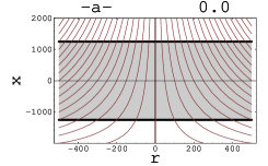
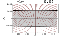
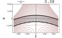
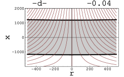
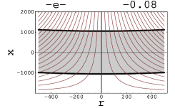
Figure 9.1: Wavefronts distribution for different values of $\xi=0.0,0.04,0.08,-0.04,-0.08$. For a clearer visualization the variable $r=10^{2}\eta$ has been used. The shady region corresponds to the strip $|x|<\frac{1}{8\beta}$ for the figure a) and $\left|P(\xi)x+Q(\xi)\eta^{2}\right|<\frac{1}{8\beta}$ for the figure b).

The three-dimensional generalization of the previous case has been discussed in the same paper [34]. In particular, from the formula (35) one gets the following real phase function at $\lambda=0$

$$\left.\hat{S}(x,\eta,\xi)\right|_{\lambda=0}=2\eta\left(P(\xi)x+Q(\xi)\eta^{2}\right)$$ (9.8)

where

$$P(\xi) = \frac{|q_{0}|\left(2p_{0}-q_{0}^{2}\right)}{q_{0}^{2}\left(q_{0}^{2}-4p_{0}\right)^{\frac{1}{2}}}-1,$$

$$Q(\xi) = \frac{8p_{0}}{3q_{0}^{2}}\left(\frac{p_{0}-q_{0}^{2}}{\left(q_{0}^{2}-4p_{0}\right)^{\frac{1}{2}}}-\frac{q_{0}^{2}\left(q_{0}^{2}-3p_{0}\right)}{|q_{0}|\left(q_{0}^{2}-4p_{0}\right)^{\frac{3}{2}}}\right),$$

$$p_{0} = 1+36\xi-\left(1-12\xi\right)^{\frac{3}{2}},~{}~{}~{}~{}~{}q_{0}=3\left(1+4\xi\right).$$

Note that for $\xi=0$ the expression for $\hat{S}$ (9.8) coincides with expression  (9.6). Moreover,the corresponding dKP solution is

$$q=\frac{4\left(5-12\xi+4\left(1-12\xi\right)^{\frac{1}{2}}\right)^{2}\left(\left(-1+12\xi\right)x-4\eta^{2}\right)}{3(1+4\xi)\left(1-12\xi+2\left(1-12\xi\right)^{\frac{1}{2}}\right)^{3}}.$$ (9.9)

Of course, expression (9.9) becomes (9.4) when $\xi=0$. We discuss the $\xi$-deformations of wavefronts in a sufficiently small neighbourhood of the plane $\xi=0$, in order to avoid $\xi$-values for which $q$ blows up or becomes complex valued.

The explicit expression of the wavefronts is the following

$$x=-\frac{\eta+2\beta Q(\xi)\eta^{2}-k}{2\beta P(\xi)\eta}$$ (9.10)

where $k$ is an arbitrary constant. The wavefronts (9.10) should be considered inside a strip given by

$$\left|P(\xi)x+Q(\xi)\eta^{2}\right|\ll\frac{1}{2\beta}.$$ (9.11)

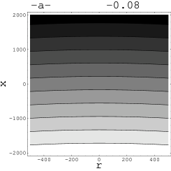
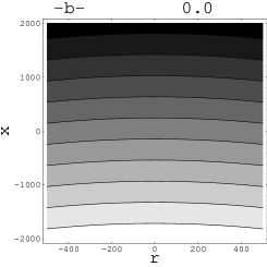
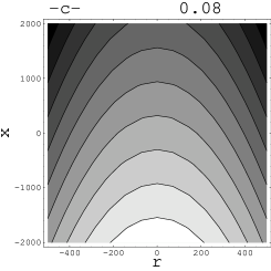
Figure 9.2: Density plot comparison of the refractive index $u$ for $\xi=-0.08,0.0,0.08$, where $r=10^{2}\eta$. Darker regions correspond to a larger refractive index.

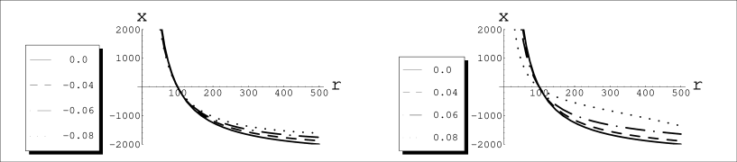
Figure 9.3: Deformation of a wavefront at different values of $\xi$.

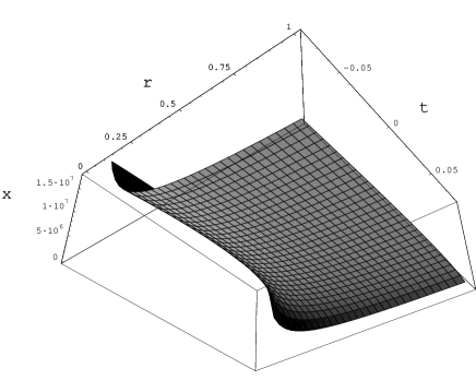
Figure 9.4: Deformation of a wavefront along the $t\equiv\xi$ direction, where $r=10^{2}\eta$. The wavefront bends in such a way that light rays turn off towards regions where the refractive index increases.

The figure 9.1 shows the wavefronts distribution inside a reasonable strip for different $\xi$-values. The figure 9.2 demonstrates that the variation of refractive index is more significant for $\xi>0$, where we observe a larger deformation of the wavefronts. One can see this in the figures 9.3 and 9.4.

9.2 dVN wavefronts.

Here, we analyze a refractive index obtained by solution of the hodograph relation (8.24), and a corresponding numerical solution of eikonal equation. Note that equation (8.24) provides us with the complex refractive index and, by consequence, the complex phase functions $S$, describing, in a way, damping effects of the electromagnetic wave (see equation (2)). Assuming $u\neq 0$ and choosing, for simplicity, $\alpha^{3}=3$, we have the following form of equation (8.24)

$$-x+iy+(x+iy)u^{2}+4x_{2}u^{5}-u^{2}\psi(u)=0.$$ (9.12)

A particular choice of the function $\psi(u)$ sets the behaviour of $u$ on the boundary $x_{2}=0$. Assuming $\psi$ polynomial on $u$, the numerical analysis shows qualitatively similar behaviours for different polynomial degrees. As particular example, we set $\psi=2u+\frac{1}{3}u^{2}$. The figure 9.5 shows the density plot of the real and imaginary parts of a refractive index $n=\frac{u}{4}$ on the transverse section $x_{2}=0$ , obtained by numerical solution of (9.12).

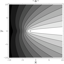
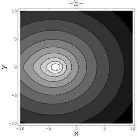
Figure 9.5: Density plot of the a) real and b) imaginary parts of the refractive index $n$ on the plane $x_{2}=0$.

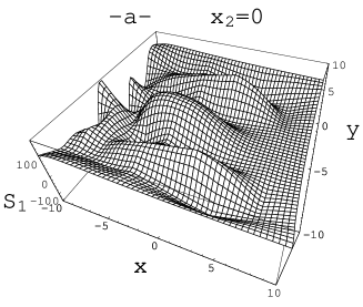
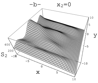
Figure 9.6: a) Real part of the phase function with boundary conditions $S_{1}(10,y)=y^{2}$ and $S_{1}(x,-10)=S_{1}(x,10)$. b) Imaginary part of phase function with boundary conditions $S_{2}(10,y)=y^{2}$ and $S_{2}(x,-10)=S_{2}(x,10)$.

Figure 9.7: Wavefront configurations associated with the real phase $S_{1}$ at different $x_{2}=0,5,10$.

Representing the phase function in terms of its real and imaginary parts, $S=S_{1}+iS_{2}$, one rewrites the eikonal equation (8.1) as the system

$$S_{1x}^{2}+S_{1y}^{2}-S_{2x}^{2}+S_{2y}^{2}=4u_{1}$$

$$S_{1x}S_{2x}+S_{1y}S_{2y}=2u_{2}$$ (9.13)

where $u=u_{1}+iu_{2}$. A numerical solution of the system (9.2) for the refractive index plotted in the figure 9.5. It has been obtained in the range $x\in[-10,10]$ and $y\in[-10,10]$ exploiting the function NDSolve of the Standard Mathematica Packages [35], with boundary conditions $S_{1}(10,y)=S_{2}(10,y)=y^{2}$ and $S_{1}(x,-10)=S_{1}(x,10)$, $S_{2}(x,-10)=S_{2}(x,10)$. The figures 9.6-a) and  9.6-b) shows $S_{1}$ and $S_{2}$ respectively. In particular, one should to note that the regions where $S_{2}$ increases, correspond to the damping of the electromagnetic wave.

Finally the figures 9.7-a)-b) and c) show the wavefronts configuration at different values $x_{2}=0,5,10$.

Acknowledgment. The authors are grateful to L.V. Bogdanov for the useful discussions.

References

- [1] R.W. Boyd, Nonlinear Optics, Academic Press, Inc., (1992).
- [2] A.S. Fokas, D.J. Kaup, A.C. Newell, V.E. Zakharov (eds.), Nonlinear Processes in Physics, Proceedings of the III Potsdam-V Kiev Workshop at Clarkson University, Potsdam NY, USA, August 1-11, 1991, Springer Verlag, (1993).
- [3] V.E. Zakharov, S.V. Manakov, S.P. Novikov and L.P. Pitaevski, The Theory of Solitons: The Inverse Problem Method, Nauka, Moscow, (1980); Plenum Press, (1984).
- [4] M.J. Ablowitz and H. Segur, Solitons and the Inverse Scattering Transform, SIAM, (1981).
- [5] P.D. Lax and C.D. Levermore, The small dispersion limit on the Korteweg-de-Vries equation, Commun. Pure Appl. Math., 36, 253-290, 571-593, 809-830, (1983).
- [6] I.M. Krichever, Averaging method for two-dimensional integrable equations, Func. Anal. Priloz., 22, 37-52, (1988); The -function of the universal Whitham hierarchy, matrix models and topological field theories, Commun. Pure Appl. Math. 47, 437-475, (1994); The dispersionless Lax equations and topological minimal models, Comm. Math. Phys. 143, 415-429, (1992).
- [7] Y. Kodama, A method for solving the dispersionless KP equation and its exact solutions, Phys. Lett. A, 129, 223-226, (1988); Solutions of the dispersionless Toda equation, Phys. Lett. A 147, 477-482, (1990); S. Aoyama and Y. Kodama, Topological Landau-Ginzburg theory with rotational potential and the dispersionless KP hierarchy, Comm. Math. Phys., 182, 185-219, (1996).
- [8] B.A. Dubrovin and S.P. Novikov, Hydrodynamics of weakly deformed soliton lattices: differential geometry and Hamiltonian theory, Russian Math. Surveys, 44, 35-124, (1989).
- [9] K. Takasaki and T. Takebe, SDIFF(2) KP hierarchy, Int. J. Mod. Phys. A Suppl., 1B, 889-922, (1992); Integrable hierarchies and dispersionless limit, Rev. Math. Phys. 7, 743-808, (1995).
- [10] Singular limits of dispersive waves, (eds. N.M. Ercolani et al.), Nato Adv. Sci. Inst. Ser. B Phys. 320, Plenum Press, New York (1994).
- [11] B.A. Dubrovin, Hamiltonian formalism of Whitham-type hierarchies and topological Landau-Ginzburg models , Comm. Math. Phys., 145, 195-207, (1992); Integrable systems in topological field theory, Nucl. Phys. B 379, 627-689, (1992); B.A. Dubrovin and Y. Zhang, Bihamiltonian hierarchies in 2D topological field theory at one-loop approximation, Comm. Math. Phys., 198, 311-361, (1998).
- [12] B. Konopelchenko and L. Martinez Alonso, -equations, integrable deformations of quasi-conformal mappings and Whitham hierarchy, Phys. Lett. A, 286, 161-166, (2001).
- [13] B.G. Konopelchenko and L. Martinez Alonso, Dispersionless scalar integrable hierarchies, Whitham hierarchy and the quasi-classical -dressing method, J. Math. Phys, 43, n.7, 3807-3823, (2002).
- [14] B.G. Konopelchenko and L. Martinez Alonso, Nonlinear dynamics on the plane and integrable hierarchies of infinitesimal deformations, Stud. Appl. Math., 109, 313-336, (2002).
- [15] Boris G. Konopelchenko, Antonio Moro, Geometrical optics in nonlinear media and integrable equations, J.Phys. A: Math. Gen., 37, L105-L111, (2004).
- [16] M. Born and E. Wolf, Principles of Optics, Pergamon Press, Oxford, (1980).
- [17] K.S. Cole and R.H. Cole, Dispersion and absorption in dielectrics, J. Chem. Phys., 9, 341-351, (1941).
- [18] L.D. Landau, E.M. Lifshitz, Electrodynamics of continuous media, Oxford, Pergamon, (1984).
- [19] John D. Jackson, Classical Electrodynamics, John Wiley & Sons, Inc., (1975).
- [20] P.C. Fannin, On the use of dielectric formalism in the representation of ferrofluids data, J. Molec. Liquids, 69, 39-51, (1996); P.C. Fannin and S.W. Charles, On the influence of distribution functions on the after-effect function of ferrofluids, J. Phys. D: Appl. Phys., 28, 239-242, (1995).
- [21] Y. Kimura, S. Hara and R. Hayakawa, Nonlinear dielectric relaxation spectroscopy of ferroelectric liquid crystals, Phys. Rev. E, 62, n.5, R5907-R5910, (2000).
- [22] B.G. Konopelchenko, Introduction to Multidimensional Integrable Equations, Plenum Press, New York and London, (1992).
- [23] I.N. Vekua, Generalized Analytic Functions, Pergamon Press, Oxford, (1962).
- [24] V.G. Veselago, The electrodynamics of substances with simultsneously negative values of and , Sov. Phys. Usp., 10, n.4, 509-514, (1968); R.A. Shelby, D.R. Smith and S. Schultz, Experimental verification of a negative index of refraction, Science, 292, 77-79, (2001).
- [25] L.V. Ahlfors, Lectures on quasi-conformal mappings, D. Van Nostrand C., Princeton, (1966).
- [26] O. Letho and K.I. Virtanen, Quasi-conformal mappings in the plane, Springer-Verlag, Berlin, (1973).
- [27] P.G. Grinevich and S.V. Manakov, Inverse scattering problem for the two-dimensional Schrödinger operator. The -method and nonlinear equations, Funkt. Anal. Priloz., 20, 14-24, (1986).
- [28] L.V. Bogdanov, B.G. Konopelchenko, Symmetry constraints for dispersionless integrable equations and systems of hydrodynamic type, arXiv:nlin.SI/0312013.SI.
- [29] E.V. Ferapontov, D.A. Korotkin and V.A. Shramchenko, Boyer-Finley equation and systems of hydrodinamic type, Class. Quantum. Grav., 19, L205-L210, (2002).
- [30] M. Mañas, L. Martinez Alonso and E. Medina, Reductions and hodograph solutions of the dispersionless KP hierarchy, J. Phys. A: Math. Gen., 35(2), 401-417, (2002).
- [31] J.-H. Chang and M.-H. Tu, Poisson algebras associated with constrained dispersionless modified Kadomtsev-Petviashvili hierarchies, J. Math. Phys., 41, no.12,8117-8131, (2000).
- [32] S. Baldwin, J. Gibbons, Hyperelliptic reductions of the Benney moment equations, J. Phys. A: Math.Gen., 36, 8393-8417, (2003).
- [33] L.V. Bogdanov, B.G. Konopelchenko and A. Moro, in preparation.
- [34] B. Konopelchenko, L. Martinez Alonso and E. Medina, Quasiconformal mappings and solutions of the dispersionless KP hierarchy, Theor. Math. Phys., 133, 1529-1538, (2002).
- [35] Wolfram Research, Inc. Mathematica 4.1 (Copyright 1988-2000).