Formation and Destruction of Autocatalytic Sets
in an Evolving Network Model
![[Uncaptioned image]](/html/nlin/0403050/assets/x1.png)
A thesis submitted for the degree of
Doctor of Philosophy in the Faculty of Science
Sandeep Krishna
Centre for Theoretical Studies
Indian Institute of Science
Bangalore - 560012, India
August 2003
Declaration
This thesis describes work done by me during my tenure as a PhD student
at the Centre for Theoretical Studies, Indian Institute of Science,
Bangalore. This thesis has not formed the basis for the award of any
degree, diploma, membership, associateship or similar title of any
university or institution.
Sandeep Krishna
August 2003
Centre for Theoretical Studies
Indian Institute of Science
Bangalore - 560012
India
Chapter 1 Introduction
In this thesis I will analyze a model of an evolving set of catalytically interacting molecules. The dynamical rules of the model attempt to capture key features of the evolution of chemical organizations on the prebiotic Earth. Such a set of molecules is an ideal example of a ‘network’ – a system of several interconnected components. The concept of a network is often used as a metaphor in describing a variety of chemical, biological and social systems, as overviewed in section 1.1. Graphs provide a natural way of representing networks in a mathematical model. I describe how a graph can be used to represent a network and the difficulties involved in creating such a representation in sections 1.2 and 1.3. Sections 1.4, 1.5 and 1.6 discuss several studies of network systems, broadly classified according to whether they focus on the structure, function or evolution of networks. This classification is not meant to be precise – several studies could be placed in more than one category. In analyzing the model I will be mainly interested in the evolution of the graph representing the chemical network. Some issues of interest are discussed in section 1.6, including the spontaneous growth of non-random graph structures, the effect of different graph structures on the selective pressures that drive the evolution and sudden mass extinctions of species. Sections 1.7 and 1.8 describe a framework for modeling an evolving network, within which some of these issues can be addressed. The specific model I will analyze will be an instance of this framework. Sections 1.9 and 1.10 mention some of the interesting phenomena observed in the model and discuss its possible use in addressing puzzles connected with the evolution of chemical networks on the prebiotic Earth. Finally, I provide a ‘map’ of subsequent chapters in section 1.11.
1.1 Networks in chemical, biological and social systems
The term ‘network’ is often used to describe a variety of chemical, biological and social systems: The metabolism of a cell is a network of substrates and enzymes interacting via chemical reactions, ecosystems are networks of biological organisms with predator-prey, competitive or symbiotic interactions, the brain is a network of interconnected neurons, and the Internet is a network of interconnected computers.
Reviews of recent work on ‘networks’ (Watts, 1999; Strogatz, 2001; Bose, 2002; Albert and Barabási, 2002; Dorogovtsev and Mendes, 2002, 2003a; Bornholdt and Schuster, 2003) testify to the diversity of systems for which the term is used:
-
•
Ecological networks: Williams and Martinez (2000), Montoya and Solé (2002) and Camacho et al. (2002) have studied a number of food webs found in freshwater, marine-freshwater interface and terrestrial environments. They have constructed graph representations of these food webs. A graph consists of a set of ‘nodes’, pairs of which may be connected by ‘links’. It is usually drawn as a set of circles (the nodes) with arrows (the links) connecting pairs of nodes. In the graph representations created by Montoya and Solé, the nodes represent species, genera and sometimes higher taxa, and links represent predator-prey interactions. Figure 1.1 shows a graph for the Ythan estuary food web. It has 135 nodes and 601 links; each link points from a species to one of its predators.
-
•
Transcription regulatory networks (Milo et al., 2002; Sengupta et al., 2002; Shen-Orr et al., 2002; Farkas et al., 2003; Maslov et al., 2003): Transcription of a gene is the process of constructing an mRNA from the DNA sequence of the gene. This process is regulated by proteins, called transcription factors, that enhance or inhibit transcription by binding to sites on the DNA, usually upstream of the gene, which in turn helps or prevents RNA polymerase and the rest of the basal transcription machinery from binding and initiating transcription. The protein product of one gene may act as a transcription factor for another gene – this network of interacting genes is called a transcription regulatory network.
-
•
Biochemical signaling networks: A number of biochemical signaling pathways exist in cells which receive and transmit information, and perform computational functions that are necessary for regulating various cellular activities. These pathways are highly interconnected, with different pathways sharing several common components, and thus forming a signaling network. One example is the mitogen-activated protein kinase network, which is involved in regulating the cell cycle (Bhalla et al., 2002).
-
•
Neural networks: The complete neural network of the nematode Caenorhabditis elegans has been mapped and can be represented as a graph with 302 nodes, each corresponding to one neuron, and more than 5000 links corresponding to synaptic or gap junction connections between neurons (White et al., 1986; Watts and Strogatz, 1998; Koch and Laurent, 1999).
-
•
Polymer chain networks: The conformation space of a lattice polymer chain can be represented as a graph, with the nodes representing possible conformations of the polymer chain and the links representing the possibility of transforming one conformation to the other through local movements of the chain (Scala et al., 2001). Sen and Chakrabarti (2001) consider a different type of network – they represent a linear polymer as a regular one-dimensional graph with nearest neighbour links and some long range links.
-
•
Metabolic networks (Fell and Wagner, 2000; Jeong et al., 2000): The metabolism of an organism, such as the bacterium Escherichia coli, is typically specified by a set of chemical reactions involving different substrates that are catalyzed by various enzymes. Figure 1.2 shows a graph of around 500 metabolic reactions. Each node represents one chemical species; a link connects two species if there is a reaction in which one species is a reactant and the other a product. This graph, unlike that in Figure 1.1, is an undirected one – the links have no associated direction and are therefore drawn as lines, not arrows.
-
•
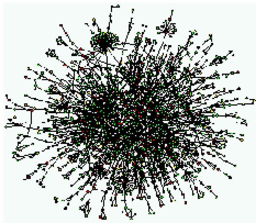
Protein interaction networks: The protein-protein interactions in the yeast Saccharomyces cerevisiae have been modeled as graphs by Jeong et al. (2001), Wagner (2001), Maslov and Sneppen (2002), Solé et al. (2002) and Vázquez et al. (2003) using data from two-hybrid assays and other experiments (Uetz et al., 2000; Ito et al., 2001). Figure 1.3 shows the protein interaction map for S. cerevisiae. In the graph each node represents a protein and an undirected link connects two proteins if they are known to interact. There are 1870 nodes and 2240 links.
-
•
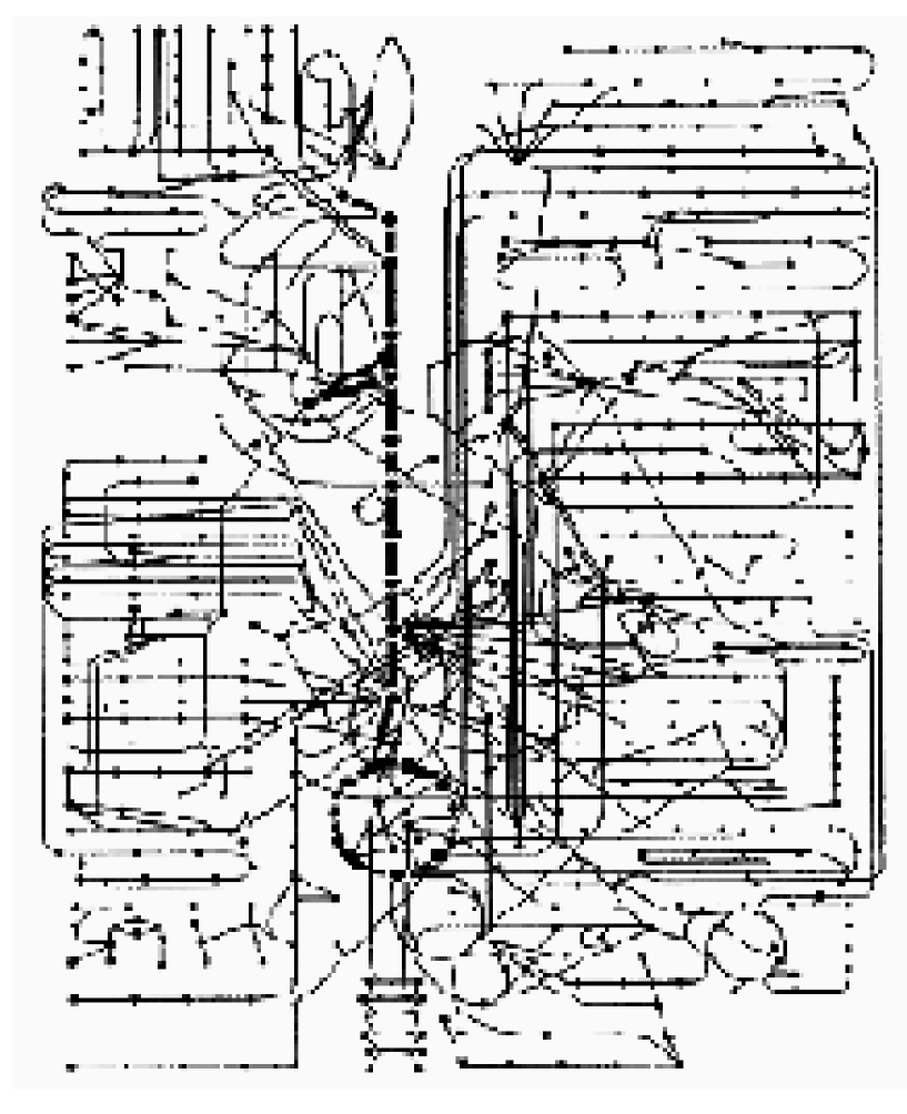
Internet: The Internet is a network of interconnected computers. Typically a few computers at one physical location (say a university or a company) are connected by a ‘local area network’. These LANs interact with each other via ‘routers’ or ‘gateways’. The topology of the Internet can be studied at various levels of detail. For example, Faloutsos et al. (1999) have studied a graph of the Internet at both the router level, where each node corresponds to a router, and at a more coarse-grained level, where each node corresponds to a group of routers. Another study of the Internet at the router level was done by Govindan and Tangmunarunkit (2000). Figure 1.4 shows a graph of the Internet at the router level. Another representation of the Internet is in terms of ‘autonomous systems’; each autonomous system “approximately maps to an internet service provider (ISP) and its links are inter-ISP connections” (Pastor-Satorras et al., 2001).
-
•
World-Wide Web: The WWW is a network of interconnected hypertext documents. The connections are in the form of ‘hyperlinks’ that can be followed to other documents on the WWW. The structure of the WWW has been studied at this level of resolution (Albert et al., 1999; Broder et al., 2000; Kumar et al., 2000) as well as at the level of ‘sites’, collections of all the documents stored on the same web server (Huberman and Adamic, 1999).
-
•
Peer to peer networks: The Gnutella network is one example. It consists of a set of computers connected to each other for the purpose of sharing files, with no central coordinating computer (Adamic et al., 2003).
-
•
Power grid networks: Watts and Strogatz (1998) have studied a graph of the electricity transmission grid of western USA. The nodes of the graph represent generators, transformers and substations, and links represent transmission lines.
-
•
Transportation networks: The Indian railway system, consisting of a network of stations connected by train services, has been studied by Sen et al. (2003). A similar network of the world’s airports has been reconstructed from data on number of passengers arriving and leaving each airport (Amaral et al., 2000).
-
•
Economic networks (Kirman, 2003): An economic system can be thought of as a network of interacting ‘agents’ (individuals, companies or even nations). Several different types of interactions can be visualized. For instance, one company may use the product of another as a raw material. In a market, individuals may interact by barter or monetary transactions. Stock market traders interact by buying and selling stocks and shares.
-
•
Word co-occurrence network: i Cancho and Solé (2001) and Dorogovtsev and Mendes (2001) have studied a graph representing the English language. The nodes represent the different words of the English language and links signify that two words occur adjacent to each other in at least one sentence in the database of texts studied. The resulting graph has approximately 470 thousand nodes and 17 million links.
-
•
Friendship networks: Amaral et al. (2000) have studied the properties of a graph representing the friendship network of a group of 417 high school students in USA.
-
•
Sexual contact network: A graph with each node representing an individual and links representing sexual contacts was constructed and studied by Liljeros et al. (2001), based on a Swedish survey of 2810 people in the age range 18-74 years.
-
•
Film actor/actress collaboration network: A graph can be constructed where nodes represent actors and actresses and a link is put between two if they have acted together in any film. Watts and Strogatz (1998) have studied such a graph of collaborations for all actors listed in the Internet Movie Database (http://us.imdb.com).
-
•
Scientific collaboration networks: A similar graph can be constructed for scientific collaborations, where nodes represent researchers and a link represents co-authorship of one or more papers. Newman (2000a, b) has studied such a graph of collaborations constructed from databases of papers in physics, biomedical research and computer science.
- •
1.2 Graph representation of a network
As is evident from the list above, the starting point of many studies is to model networks using graphs. A graph representation is useful for formulating questions about the structure and functioning of a network more precisely. Graph theory suggests several quantities that can characterize the structure of a graph. These can be computed for a real network and used for comparison with, for instance, random and regular graphs.
The correlation of these graph theoretic quantities with the functioning of the network can also be studied, thus exposing, in a more precise way, the connection between a network’s structure and its functioning. Another possibility a graph representation allows is of a cross comparison of very different systems – for instance, the metabolic network of a cell can be compared with the Internet.
In many natural systems, the network of interactions is itself a dynamical variable: The transcription regulatory network of an organism changes as genes evolve, the World Wide Web changes as web pages get added and deleted, and ecosystems change as species become extinct and new species arise. With a graph representation of the network, one can model processes that alter the graph with time, either in discrete steps or continuously.
1.3 Difficulties of creating a graph representation
Representing a network as a graph is not as straightforward as it may seem at first glance. Firstly, it is likely that several different graphs can be drawn for a given system, each of which focus on different aspects of the network. Consider, for example, the metabolism of the bacterium Escherichia coli, which is specified by a set of chemical reactions involving different substrates that are catalyzed by various enzymes. Fell and Wagner (2000) construct two different graphs from this information. The ‘reaction graph’ has a node for each chemical reaction with a directed link from one reaction to another if a product of the first reaction is used as a reactant for the second. The ‘substrate graph’ has one node for each substrate with a directed link from one substrate to another if there is a reaction in which the first substrate is a reactant and the second a product. Jeong et al. (2000) represent the metabolic network of each of 43 organisms as a graph consisting of two types of nodes, one type for each substrate and one type for each reaction. The graph is bipartite with links from substrate nodes to reaction nodes and reaction nodes to substrate nodes but no links connecting two substrate or two reaction nodes. This graph has more information than the previous two but also leaves out some information, for example, the stoichiometry of the reactions. Thus, each of these three types of graphs encodes different information about the metabolic network, and each of them excludes certain information.
Another problem is the incompleteness and uncertainty of data (Kohn, 1999). When the system consists of a complex network of interactions, even a single missed interaction or an erroneously added interaction, can drastically affect the dynamics. Food webs tend to suffer from a bias against including parasites (Williams and Martinez, 2000). Incompleteness of data is suggested by Williams and Martinez (2000) and Camacho et al. (2002) as one of the possible reasons why the Ythan estuary food web appears to differ, in several properties, from the other food webs they have studied. Protein interaction networks are another example. The two hybrid experiments that have been used to build these networks are susceptible to both false positives as well as false negatives, i.e., some protein interactions may be erroneously missed and some non-existent protein interactions may be included (Uetz et al., 2000; Ito et al., 2001).
1.4 Structure of networks
How can one characterize the structure of the Internet, the neural network of Caenorhabditis elegans, or the Indian railway system? Representing a network as a graph makes it possible to use various graph theoretic measures to characterize its structure. For instance, one can compute the length of the shortest path between two nodes averaged over all pairs of nodes in the graph. This quantity can be compared with that expected for a ‘random graph’. Random graphs – graphs where each pair of nodes has a probability, , to be connected by a link (see section 2.9 for a more precise definition) – were introduced by Erdős and Rényi (1959), and have several known structural characteristics. In the limit where the number of nodes of the graph, , tends toward infinity, then if (equivalently, if the number of links ) the graph consists of several connected clusters of nodes, each of which has only a finite number of nodes, and if (or ) a ‘giant’ connected cluster exists which has an infinite number of nodes (Bollobás, 2001). The average shortest path length for an undirected random graph of nodes, with enough links to contain a giant cluster, grows as (Bollobás, 2001). At the other extreme are regular graphs, such as a one-dimensional chain of nodes whose average shortest path length scales in proportion to (for a -dimensional hyper-cubic lattice it would scale as ).
Graphs of the Indian railway network (Sen et al., 2003), the western USA power grid network, the movie actor network, the neural network of C. elegans (Watts and Strogatz, 1998), the world airport network and polymer chain networks (Amaral et al., 2000), and ecological networks (Montoya and Solé, 2002) are known to have low average path lengths similar to random graphs with the same number of nodes and links.
However they differ from random graphs in other characteristics, like ‘clustering’. A set of nodes is ‘clustered’ if in some sense the nodes are more ‘strongly connected’ to each other than to other nodes of the graph outside the set. One measure of the amount of clustering in a graph is the ‘clustering coefficient’, which is the probability that two neighbours of any node are also neighbours of each other. Regular graphs have a relatively large clustering coefficient, while random graphs have a relatively low coefficient.
The networks mentioned above, which have a low average path length, have much higher clustering coefficients than random graphs with the same number of nodes and links. Graphs of this type which have a comparable average path length but a much higher clustering coefficient than a similar random graph have been dubbed ‘small-world’ graphs (Watts and Strogatz, 1998; Watts, 1999).
Another measure is the degree distribution of a graph. The degree of a node (the total number of outgoing and incoming links to a node, see section 2.2) takes a range of values over all the nodes of any graph. The distribution of these values can be analytically calculated for the random graph described above, and is a binomial distribution. Given a graph of a real network, say the Internet, one can compute its degree distribution and compare with the binomial distribution expected for a random graph with the same number of nodes and links. In contrast, a regular graph, such as the lattice of a crystal solid, has nodes whose degrees take at most a few different values. For example, in a body-centred cubic lattice (such as that formed by iron or CsCl) each node (atom) has a degree eight. Many networks, such as the metabolic network of E. coli (Jeong et al., 2000), the Internet (Faloutsos et al., 1999) and citation networks (Seglen, 1992; Redner, 1998) have neither the binomial degree distribution of a random graph nor the discrete distribution of a regular graph. Instead their degree distribution has a power law tail. Such networks have been termed ‘scale-free’ (Barabási and Albert, 1999). Montoya and Solé (2002) claim that ecological networks also have a scale-free degree distribution, a conclusion that is disputed by Camacho et al. (2002). Several properties of scale-free graphs have been elucidated (Newman et al., 2001; Bollobás and Riordan, 2003). For instance, scale-free graphs are small-world, having a small average shortest path length (Barabási and Albert, 1999) and a high clustering coefficient (Watts, 1999). However, the converse is not true: Amaral et al. (2000) show that not all small-world networks are scale-free – among several different networks that are small-world, the degree distribution of some have an exponential tail like random graphs, some are scale-free, while others have a power-law distribution which is truncated by an exponential or a gaussian tail.
Yet another measure used to characterize a graph is its eigenvalue spectrum. Any graph with nodes can be specified by an ‘adjacency’ matrix. The collection of eigenvalues of this matrix is the eigenvalue spectrum of the graph. Some structural characteristics of a graph are reflected in the eigenvalue spectrum. For instance, in a directed graph, the largest eigenvalue is directly related to the presence or absence of cycles in the graph (see section 2.8). Though only some aspects of the connection between the spectrum and the structure of the graph have been worked out, it nevertheless serves to classify graphs into different groups. Once again, some properties of the spectrum of a random graph are known. For an undirected random graph, with enough links to contain a giant cluster, the value of the largest eigenvalue scales as , when , while the distribution of the rest of the eigenvalues converges to a semi-circle whose width is proportional to (Farkas et al., 2001). Therefore, the amount by which the eigenvalue spectrum of a real network deviates from this ‘semi-circle law’ is a measure of the non-randomness of the graph. Farkas et al. (2001) and Goh et al. (2001) have shown that the eigenvalue distributions of sparse random graphs and scale-free graphs are very different from the semi-circle distribution.
The clustering and degree of a node are ‘local’ quantities, in the sense that they depend only on the immediate links of the node or at most the links of its neighbours. In contrast, shortest path lengths, eigenvalues and eigenvectors are ‘non-local’ quantities, in the sense that the shortest path between two nodes, or the component of an eigenvector corresponding to a node, depends on the entire graph and not just on the immediate links of the nodes in question. It is therefore not surprising that the possibility of missing or extra links is a more serious problem for the non-local quantities than for the local quantities. The addition or removal of a small number of links will not significantly affect the degree distribution or the clustering coefficient. In contrast, adding a small number of random links to a regular graph reduces the average path length drastically (Watts and Strogatz, 1998). Similarly, the addition of a single link can create a cycle, where there was none before, thereby changing the largest eigenvalue.
Another non-local graph-theoretic measure is the dependency of a node, which, for a directed graph, is defined to be the number of links that lie on paths leading to the node in question (Jain and Krishna, 1999). The average dependency of nodes of a graph is termed the ‘interdependency’ of the graph because it is a measure of how interdependent are the nodes of the graph. Section 2.2 will discuss more about these measures.
A structural characteristic that is of interest, especially for chemical networks, is the property of autocatalysis. The concept of an autocatalytic set of chemical species was introduced by Eigen (1971), Kauffman (1971) and Rossler (1971), and is defined in that context to be a set of molecular species that contains, within itself, a catalyst for each of its member species. This notion is closely related to that of positive feedback loops and can be generalized to different systems which have other kinds of ‘beneficial’ interactions – for instance, symbiosis in ecological networks. Hong et al. (1992) and Lee et al. (1997) have each constructed a pair of different molecules that catalyze one another’s (as well as their own) production and hence form an autocatalytic set of this kind. Wächterhäuser (1990) and Morowitz et al. (2000) use a slightly different, but related, definition of autocatalysis to argue that the reductive citric acid cycle is autocatalytic. A graph-theoretic definition of autocatalytic sets (Jain and Krishna, 1998) is discussed in section 3.1. Autocatalytic sets will play a major role in the dynamics of the model studied in this thesis.
Several other structural characteristics of graphs that have this non-local character have been studied: Dhar et al. (1987) have analyzed the structure of the shortest path spanning all nodes in a variety of graphs derived from regular lattices; Janaki and Gupte (2003) define the “weight-bearing capacity” of a branching hierarchical network and analyze which network structures enhance this capacity; Hartwell et al. (1999) and Lauffenburger (2000) argue that cellular networks are ‘modular’, i.e., consisting of distinguishable clusters of nodes that play some functional role; Ravasz et al. (2002) suggest that the metabolic network of E. coli may have a hierarchical structure; Milo et al. (2002), Shen-Orr et al. (2002) and Maslov et al. (2003) describe a way of decomposing the transcription regulatory network of E. coli into commonly occurring ‘motifs’, which are specific patterns of connections between a small set of nodes.
1.5 Dynamical systems on networks
A different set of questions about such networks concerns the dynamics of variables ‘living’ on the graph – for example, the concentrations of different chemical substrates in a cell, or the populations of species in an ecosystem, or the number of times a document on the WWW is accessed. The network topology affects the dynamics of these variables. The food-web structure of an ecosystem affects the dynamics of its constituent species’ populations; the network of human contacts influences the spread of a contagious disease.
Such dynamical systems on networks are often modeled as a set of coupled differential equations in which the couplings are specified by the network of interactions. An example is a network of coupled (possibly nonlinear) oscillators where one common question asked is whether groups of oscillators eventually synchronize despite different natural frequencies and initial phases. The synchronization properties of coupled dynamical systems have been studied for network structures ranging from a fully connected graph (Strogatz, 2000) to regular lattices (Kaneko, 1989; Pérez et al., 1996), to trees (Gade et al., 1995), and a variety of sparse network structures (Jalan and Amritkar, 2003; Sinha, 2002). Ramaswamy (1997) has described the synchronization of coupled strange non-chaotic attractors. The stability of the synchronization to perturbations of the coupling strengths has been studied by Chen et al. (2003) for a large class of coupled maps and differential equations.
In ecosystem models, the Lotka-Volterra equation, replicator equation and other more complicated differential equations have been used to represent the dynamics of the populations of species (Drossel and McKane, 2003). The replicator equation, for example, displays a range of different behaviour depending on the network structure – fixed point, limit cycle, heteroclinic cycle and chaotic attractors have been observed (Hofbauer and Sigmund, 1988). Biochemical signaling networks too exhibit a variety of dynamics (Bhalla and Iyengar, 1999; Bhalla, 2002).
The dynamics of neural networks has been extensively studied. One example is a model of a neural network that exhibits a periodic cycling between different meta-stable states (“memories”) as well as intermittent transitions to a high activity state resembling epileptic seizures (Biswal and Dasgupta, 2002a, b). Sinha and Chakrabarti (1999) review what is known about synchronization in neural network models. For a comprehensive review of neural network models see (Arbib, 1995).
Some dynamical systems on networks have the property of displaying a variety of different dynamics even for the same network topology. Suguna et al. (1999) describe a simple model of a biochemical pathway that can show fixed point, periodic, birhythmic and chaotic dynamics as the rates of the reactions comprising the pathway are changed, while keeping the topology of the pathway fixed. Bhalla et al. (2002) analyze a biochemical signaling pathway whose dynamics is either monostable or bistable depending on the parameter values.
In some systems it is more appropriate to represent the dynamics by difference equations, rather than differential equations, or by cellular automata. This is especially true for systems where the variables of interest take discrete values and assuming them to be continuous variables is a bad approximation. For instance, models of traffic on transportation networks in which particles (vehicles) are individually represented often show a different behaviour (e.g., different phase transitions from a free flowing state to a traffic jam state) from models in which a continuous traffic flow rate is the dynamical variable. Nagel (2003) reviews different traffic models on various types of networks. Several studies of neural networks model the neurons as cellular automata (Arbib, 1995). Two studies where the dynamics occurs in discrete time steps are described by Pandit and Amritkar (2001), who have studied the dynamics of random walkers on a class of small-world networks, and Dube et al. (2002), who have studied the effect of different pricing schemes on the dynamics of queues of people accessing an Internet web server.
When the dynamics can be assumed to be reaching some steady state or fixed point, there may be short cuts to finding the steady state without actually having to solve the equations of motion. For instance, Edwards et al. (2001) describe a procedure for determining the rates of the chemical reactions comprising the intermediary metabolism of E. coli, assuming a steady state. Instead of finding the rates as the attractor of some difference or differential equations, the procedure is based on linear optimization of a specifically chosen function under the constraints imposed by the stoichiometry of the reactions. The structure of the steady state reaction fluxes can be studied as a function of different network topologies.
Local search strategies are another example of dynamical systems on a network (Adamic et al., 2003). The Gnutella file sharing system consists of a network of computers; there is no central coordinating computer that has information about the entire network, in particular, which files are available at which nodes. Therefore, each user must use a local search strategy, an algorithm that uses only local information, such as the identities and connections of a particular node’s neighbours, its neighbour’s neighbours, etc., to find where a particular file is located on the network. Again, the network topology is crucial because, for example, the most efficient search algorithms for regular graphs are quite different from those for random or scale-free graphs (Adamic et al., 2003).
Another set of studies involving dynamics on networks is in the field of epidemiology. In the models studied by Watts and Strogatz (1998) and Pastor-Satorras and Vespignani (2003) diseases spread faster in small-world or scale-free graphs than in regular and random graphs. Similar models are used to study the spread of computer viruses through the Internet. These models can suggest efficient immunization techniques by identifying which links or nodes of the graphs are contributing most to the spread of the virus (Pandit and Amritkar, 1999; Pastor-Satorras and Vespignani, 2003).
Closely related to this are studies of ‘attacks’ on a network by the removal of nodes of the network. Albert et al. (2000), Callaway et al. (2000) and Cohen, R., et al. (2000, 2001) show that scale-free networks are more robust to random attacks than random graphs but are susceptible to directed attacks at the nodes with the highest degree. These studies contain networks that are changing with time, though the dynamics simply involves nodes getting removed in a specified order. The next section deals with studies of evolving networks with more complicated dynamics.
1.6 Evolution of networks
So far I have focused mainly on the structure of, and the behaviour of dynamical systems on, fixed networks. However, real networks are rarely static. An obvious question, therefore, is how (and why) did a particular network evolve into the specific structure we see? For instance, has the structure of a network evolved to optimize certain functionality? Further, one can ask what are the mechanisms that cause the network to change? Is the evolution driven by Darwinian natural selection, or Lamarckian selection, or by other self-organizing processes?
Some of the structural and dynamical studies in the previous two sections can be used to make some guesses about the evolution of the network. For instance, Fell and Wagner (2000) suggest that the small-world structure of metabolic networks may have evolved to enable a cell to react rapidly to perturbations. Watts and Strogatz (1998) suggest that the visual cortex may have evolved into a small-world architecture because that would aid the synchronization of neuron firing patterns. The robustness of scale-free networks to random removal of nodes has been suggested as an evolutionary reason for the prevalence of scale-free networks (Albert et al., 2000).
While studies of static networks do provide some insight into network
evolution, it is natural to address such evolution-related questions
in models where the network is also a dynamical variable. One possibility
is to analyze a variety of simple models of changing networks, with
different rules governing the dynamics of the network, and see which
rules produce structures like small-world or scale-free graphs that
are commonly observed in real networks: Watts and Strogatz (1998) describe a model
that produces a small-world graph by randomly rewiring or adding links
to a regular graph. A similar model (where the number of nodes is
fixed but links are repeatedly added) that produces scale-free networks,
is described by Mukherjee and Manna (2003). Several other ‘growing network’ models
start from an empty network and add nodes and links at discrete time
steps. The ‘preferential attachment’ rule – new nodes are preferentially
assigned links to nodes with a high degree – produces scale-free
graphs (Barabási and Albert, 1999). Albert and Barabási (2002) and Dorogovtsev and Mendes (2002) review several different
models of this type, using both deterministic and stochastic rules,
that give rise to scale-free graphs. The growing network model described
by Manna (2003) adds another level of complexity by making the addition
of new links to the network dependent on the dynamics of several random
walkers on a regular lattice. Variants of these models exist where
the preferential attachment to nodes of high degree competes with
the preferential attachment to nodes of a lesser age, i.e., nodes
that have been added to the network more recently. Amaral et al. (2000) have
shown that such aging effects can result in a graph whose power-law
degree distribution is truncated by an exponential tail. Dorogovtsev and Mendes (2003b)
discuss models of accelerated growth of networks, where the rate of
addition of new nodes increases with time. Williams and Martinez (2000) describe a simple
set of rules to grow a network, that produces graphs remarkably similar
in structure to many ecological food webs (Camacho et al., 2002).
One aspect missing from these growing network models is that the dynamics of the network is not intertwined with the dynamics of other variables. The models that include aging are implicitly using a dynamical variable, the age of a node, but the dynamics of that variable is not coupled to the structure of the graph. In many natural systems the dynamics of the network is tightly coupled to the dynamics of the variables living on it, and vice versa. For example, a food-web influences the dynamics of the species’ populations, and if a species becomes extinct, the food-web changes. The firing pattern of neurons depends on the structure of the neural network and the strengths of synaptic connections are in turn modified by the repeated firing or non-firing of neurons (Arbib, 1995). There exist a number of models that incorporate this feature too. Models of learning and memory in neural networks typically have neuron firing patterns co-evolving with the network connection strengths (Arbib, 1995). A number of such evolving ecosystem models have been studied (Lindgren and Nordahl, 1994; Solé and Manrubia, 1996; Chowdhury et al., 2003) (see Drossel and McKane, 2003, for a review). Evolving replicator networks have been described by Happel and Stadler (1998) and Tokita and Yasutomi (2003).
In addition to creating evolving network models that produce graphs having a similar structure to existing networks, one can also use evolving network models to address a number of other evolution-related questions. For instance, how does the existing structure of a network influence its subsequent evolution? This question is best addressed in a model where the evolution of the network is coupled to the dynamics of other variables, which, in turn, are affected by the network structure. Because of this coupling, the different (sub)structures in the network affect its evolution. For instance, autocatalytic sets in prebiotic chemical networks might have been more stable to perturbations because of their ability to self-replicate. If so, an interesting question is: Can such stable structures grow, or spread through a network and, if they can, over what timescales? Further, one can ask how the existing structures determine the short and long term effects of a perturbation on the evolution of the network; in an ecosystem, whether an invading species will be able to survive, and for how long, will depend on the competition and resources provided by the existing species.
A related set of (meta)questions can be asked about the ‘evolvability’ of networks. Kirschner and Gerhart (1998) have defined the evolvability of a biological organism as the capacity to generate heritable, selectable phenotypic variation. This definition can be extended to other types of networks. Then one can ask: How evolvable is a network? Is this evolvability also subject to selection and has it, therefore, itself evolved over time?
One of the inspirations for the model I will discuss in this thesis are the models of Kauffman, Farmer, Fontana and others who have explored questions about self-organization, the origin of life and some of the above evolvability issues in work on artificial chemistries. An artificial chemistry is a system whose components ‘react’ with each other in a way analogous to molecules participating in chemical reactions. Thus, Kauffman (1983) and Bagley et al. (1991) consider systems composed of strings of arbitrary length made from a binary alphabet. Strings can participate in ‘cleavage’ and ‘ligation reactions’ which involve the splitting or concatenation of strings to form new ones. Just as with a real chemistry, not all reactions will be allowed and there are different ways of specifying which strings participate in which reactions. The simplest way is to randomly decide which reactions are allowed, resulting in a ‘random chemistry’ of the type studied by Kauffman. He found that there is a critical number of links, such that if a random chemistry has more than that number of links, it is almost certain to contain an autocatalytic set (Kauffman, 1993).
Bagley et al. (1991) have explored an artificial chemistry consisting of catalyzed ligation and cleavage reactions. Their network evolves with time as new molecules can be created by the ligation of existing ones. They address the puzzle of how large molecules with highly specialized functionality, like enzymes and DNA, could have evolved from an initial condition that contained only small molecules which interacted weakly and non-specifically. Again, autocatalytic sets play an important role in the overall dynamics and are suggested as one of the possible means by which a complex chemical organization, a ‘metabolism’, could have evolved on the prebiotic Earth. Fontana (1991) and Fontana and Buss (1994) study more abstract artificial chemistries consisting of functions expressed in the lambda-calculus. Each function can ‘react’ with other functions, producing a new function by the composition of the ‘reactant’ functions. They find that in such a chemistry there is a spontaneous emergence of groups of cooperative reactions such as self-replicators, self-replicating sets, autocatalytic cycles, symbiotic and parasitic functions.
If Darwinian natural selection is driving the evolution of the network one can ask, what were the selective pressures acting on the network at different times? How do the selective pressures change with the structure of the network? Whenever the dynamics of the network has a stochastic component the detailed structure of the network is typically a result of many chance events. Nevertheless, some patterns may still be predictable. Thus, it is of interest to ask which patterns are predictable and which are a result of historical accidents.
Another aspect of the dynamics of evolutionary systems is the destruction of structures. In evolving systems, non-random structures not only emerge but also get destroyed in some circumstances. A number of mass extinctions are documented in the fossil record (Newman and Palmer, 1999). Financial markets suffer sudden large crashes (Bouchaud, 2001; Johansen and Sornette, 2001). Discovering markers that can be used to predict an imminent crash would obviously be very useful in the context of financial markets. It is of interest to try to identify the possibly multiple causes of such crashes. Many mechanisms have been suggested to explain mass extinctions in the fossil record (Maynard-Smith, 1989; Glen, 1994). The model of Bak and Sneppen (1993) is one example of attempts to explain the distribution of extinction sizes. Tokita and Yasutomi (1999) have studied various statistical properties of the extinction events in their model of an ecosystem. In ecosystems there can exist ‘keystone’ species whose extinctions are likely to trigger a cascade of further extinctions (Paine, 1969; Jordán et al., 1999; Solé and Montoya, 2001). This raises several interesting questions: Knowing the structure of an ecological network can one predict which species are keystone? Are there any mechanisms that exist to ‘protect’ such important species?
In this thesis I will try to address some of these issues within the context of a specific mathematical model of an evolving network. Many of the phenomena exhibited by the model are reminiscent of the phenomena seen in a variety of evolving networks – the growth of non-random structure (in the form of autocatalytic sets), the growth of interdependence and cooperation between nodes of the network, sudden mass extinctions due to the extinction of keystone species or the creation of certain new structures in the network (termed ‘innovations’). The model provides a simple mathematical framework within which to analyze the mechanisms that produce such phenomena. The basic model, and its variants, will be specific instances of a broad framework for modeling evolving networks that I present in the following section.
1.7 Framework of a model in which the network co-evolves with other variables
Consider a process that alters a network, represented by a graph, in discrete steps. The series of graphs produced can be denoted . Each step of the process, taking a graph from to , will be called a ‘graph update event’. The following framework defines a class of evolving network models that consist of a graph evolving, by a series of graph update events, along with other system variables:
- Variables:
-
The dynamical variables are a directed graph and a variable associated with each node of the graph. For example, could represent:
-
•
the concentrations of substrates and enzymes in a metabolic network,
-
•
the expression level of genes in a genetic regulatory network,
-
•
the populations of species in an ecosystem,
-
•
the state (firing or not firing) of neurons in the brain,
-
•
the number of times each web page on the world wide web has been accessed,
-
•
the number of films each actor/actress has worked in,
-
•
the profits of each of a set of interacting companies.
- Initialization:
-
To start with, the graph and the variables are given some initial values. The particular choice of values will depend on the system being modeled.
- Dynamics:
-
Step 1:
First, keeping the graph ( at step ) fixed, the are evolved for a specified time according to a set of differential equations that can be schematically written in the form: , where are certain functions that depend upon the graph and on all the variables.
-
Step 2:
After this, some nodes may be removed from the graph, along with their links. Some links may also be removed from the graph. Which nodes and links are removed will, in general, depend on the values of the nodes and the graph .
-
Step 3:
Similarly, some nodes may be added to the graph. These new nodes will be assigned links with existing nodes. The rules for specifying which links will be assigned may depend on the values of the other nodes and . The new node will be given its own variable, which will be assigned some initial value. Some new links may be added between existing nodes, which again may depend on the values of the nodes and .
Steps 2 and 3 produce a new graph which will be the graph at time step , . This process, from step 1 onward, is iterated.
The above provides a nonequilibrium statistical mechanics framework for a model of an evolving network. The graph is generically in a nonequilibrium state because of the constant flux of nodes and links into and out of the graph. The variables may also be in a nonequilibrium state depending on the form of of . The graph dynamics in this framework is a specific case of a Markov process on the space of graphs. For a general Markov process, at time , the graph determines the transition probability to all other graphs. The stochastic process picks the new graph for time , , using this probability distribution. In the example here, the transition probability is not specified explicitly. It arises implicitly as a consequence of the dynamics of the variables (step 1) and the way the specified rules for steps 2 and 3 use the values to determine which nodes and links will be removed or added.
There are two timescales built into this framework. On a timescale much shorter than , the variables can evolve while the graph remains fixed. On a longer timescale, the graph changes in discrete steps that involve the possible removal and addition of nodes and links. The operation of the dynamics and the graph dynamics on different timescales is common to many systems. In the brain, over short times neurons fire or not depending on their fixed synaptic connections and the firing of other neurons, while over a long timescale the firing pattern can cause the synaptic connections to strengthen or weaken. In an ecosystem, over short timescales the species composition is fixed while the populations change, and over long times the network changes because of the extinction and mutation of existing species and the invasion of the system by new species. In a genetic regulatory network, over short times the genes and regulatory interactions are fixed and it is the expression level of genes that changes with time, and on a longer timescale the genes themselves evolve. These examples also reiterate what was mentioned before – the dynamics and the graph dynamics are interdependent. This feature is also built into the above framework: The dependence of the dynamics on the graph lies in the dependence of the functions on . The dependence of the graph dynamics on lies in steps 2 and 3. The particular choices of as well as the rules determining which, if any, nodes and links will be removed or added will depend on the particular system that is being modeled.
1.8 Extensions of the framework
This framework can be extended to include a larger class of evolving network models. Firstly, as mentioned in section 1.5, it may be preferable to model some systems using difference equations or cellular automata. For instance, if the populations of all species in an ecosystem can be assumed to be large then treating them as continuous variables and representing their dynamics by differential equations may be reasonable. But if the populations are close to zero this could be a bad approximation. It is easy to alter step 1 to take into account these possibilities. Secondly, it may be more appropriate to model some systems using two or more graphs, or by some generalization of a graph like a hypergraph. For example, in a cell, the metabolic network is linked to the genetic regulatory network and the dynamics on one network can affect the dynamics on the other. A number of neural network models of learning consist of two interacting networks, the ‘teacher’ and the ‘student’; Kinzel (2003) has reviewed several models that consist of more than one neural network interacting with one another. The framework described above can be generalized to deal with such systems: Kohn (1999) has described a generalized form of a graph that he uses to represent all the different types of interactions in the mammalian cell cycle control and DNA repair systems. Thirdly, as is the case in some neural network models (Arbib, 1995), it may be worthwhile to consider dynamical rules where the network changes continuously with time, rather than in discrete steps as in the above framework.
1.9 The origin of life: evolution of a chemical network
In this thesis I will describe a model – a particular instance of the above framework – whose rules attempt to describe some aspects of the dynamics of a chemical network in a pool on the prebiotic Earth (Jain and Krishna, 1998). Assume that the pool contains many amino acid monomers or nucleotide bases, as well as some small polypeptide chains or short RNA molecules which may have a weak catalytic activity (Joyce, 1989). For instance, some of these polypeptides or catalytic RNA might catalyze the production of other polypeptides or RNA from the monomers present in the pool. Such a chemical network can be represented as a graph in which the nodes are the polypeptides/RNA and the links represent their catalytic interactions. This would be the graph in the model. The could represent the concentrations or relative populations of each type, or species, of polypeptide or RNA. would change with time as the possible chemical reactions proceed to produce or deplete the different molecular species. Focusing only on the catalyzed reactions which produce different molecular species from the monomers, one can imagine that for a short timescale, over which the pool remains undisturbed, the chemical network (i.e., ) will be fixed with no molecular species entering or exiting the pool. Thus, the will evolve according to the chemical rate equations, with fixed. In section 4.1, I derive the form of for such chemical rate equations under the following assumptions:
-
•
only reactions involving the catalyzed production of each molecular species are modeled,
-
•
the catalyzed reactions are described by the Michaelis-Menten theory of enzyme catalysis,
-
•
the Michaelis constants for each reaction are very large compared to the populations,
-
•
the concentrations of all the required reactants are non-zero and fixed,
-
•
all catalysts have the same strength,
-
•
the pool is well-stirred, i.e., there are no spatial degrees of freedom.
Over long timescales imagine that the pool is subject to perturbations in the form of floods, tides or storms which may flush out part of the pool and possibly introduce new molecules into the pool. Removing a node from the graph would correspond to removing all the molecules of a particular type from the pool. When a perturbation removes a random lot of molecules, the molecular species with smaller are more likely to be completely wiped out from the pool. For step 2, I will choose a rule that implements an extreme version of such selection: the node with the least will be removed along with all its links. A perturbation can add a new node to the graph, with a small value. An added node corresponds to a new type of molecule being brought into the pool by the perturbation. As there is no reason to assume such a node would have any particular relationship with existing nodes it is reasonable to assign the links of the new node randomly. Therefore, for step 3, I choose the rule: add one new node, whose links with existing nodes are assigned randomly. In this scenario one can assume that the perturbation would not remove existing links without removing a node, or create a new link between existing nodes. Therefore, these possibilities can be excluded from the model. A detailed description of the model rules is given in chapter 5.
Such a model could address some questions concerning the origin of life on Earth (Jain and Krishna, 2001). The chemical network of a bacterial cell of today consists of several thousand types of molecules involved in thousands of different chemical reactions. Each type of molecule plays a definite functional role and the entire chemical network is organized to enable the cell to perform the various functions it needs to survive and reproduce in often extreme conditions. This chemical organization is highly non-random – the molecules found in cells are a small subset in a very large space of possible molecules and the graph that describes their interactions is a special kind of graph in the very large space of graphs. The probability of such a structured chemical organization arising by pure chance is extremely small. After the oceans condensed about 4 billion years back on the prebiotic Earth there was no such chemical network of interactions existing anywhere. However, if we assume that life originated on Earth about 3.5 to 3.8 billion years ago as suggested by the microfossil evidence (Schopf, 1993), then that leaves a few hundred million years for the first living cells to form. A puzzle of the origin of life on Earth is: how did such a structured, non-random chemical organization form in such a short time? This question can be addressed in the above model. One can start with a random graph, representing the situation just after the oceans would have condensed on Earth, where the pool would be likely to contain a random set of molecules with no particular non-random chemical organization. As I will show, starting from this initial state, the chemical network in the model described above evolves inevitably into a highly non-random, autocatalytic network (Jain and Krishna, 1998, 1999). The mechanisms that cause this growth might throw light on the above puzzle.
1.10 Catastrophes and recoveries in evolving networks
The model I will analyze also exhibits sudden catastrophes – mass extinctions where the relative populations of many species fall to zero in a short time – which are followed by slow recoveries. The asymmetry between catastrophe and recovery times, and fat tails in the size distribution of catastrophes in the model (Jain and Krishna, 2002a) are also observed in catastrophes and recoveries seen in the fossil record (Newman and Palmer, 1999) and in financial markets (Bouchaud, 2001; Johansen and Sornette, 2001). The mechanisms that cause such mass extinctions are a matter of much debate (Maynard-Smith, 1989; Glen, 1994). The model of Bak and Sneppen (1993) is an attempt to explain the frequency distribution of extinction events of different sizes using the mechanism of self-organized criticality. The model I will study is similar in some ways to the Bak-Sneppen model, with the addition of another dynamical variable – the network structure of the system. The advantage of explicitly modeling the network structure is that the mechanisms causing the catastrophes and their dependence on the network structure can be analyzed in detail.
I will show that, in the model, the largest extinctions are caused mainly by three mechanisms (Jain and Krishna, 2002b). One of the mechanisms involves the removal of specific species. This is reminiscent of the notion of ‘keystone species’ that was discussed in section 1.6. Thus, in this model, one can give a graph-theoretic definition of keystone species and explain why their removal causes mass extinctions (Jain and Krishna, 2002b).
1.10.1 Innovations
Apart from the removal of species, it is interesting that ‘innovations’ – the creation of new structures in the network – can also cause catastrophes. In the context of the model it is possible to create a graph-theoretic definition for the term ‘innovation’ (Jain and Krishna, 2002b, 2003b). This definition allows me to construct a hierarchy of innovations and correlate the graph-theoretic structure of an innovation to its short and long term effects on the evolution of the network (Jain and Krishna, 2003a, b).
1.11 A map of subsequent chapters
Chapters 2–4 describe different segments of the basic model, that are put together in chapter 5, and introduce various results from graph theory that will be useful for analyzing the model. The later chapters analyze the diverse phenomena observed in the model using the results from the previous chapters. In more detail:
- Chapter 2
-
introduces certain elements of graph theory. I set out the notation that will be used and give definitions of directed graphs, degree of a node, paths, cycles and connected components of a graph. I introduce the notions of ‘dependency’ of a node, and ‘interdependency’ of a graph. I define the Perron-Frobenius eigenvalue and eigenvectors of a graph and describe some of their properties. Random graphs are briefly discussed at the end of the chapter.
- Chapter 3
-
introduces the concept of an ‘autocatalytic set’. I describe the relation between algebraic properties of a graph, such as the Perron-Frobenius eigenvalue and eigenvectors, and topological properties, such as the presence or absence of autocatalytic sets in a graph. I then present the eigenvector profile theorem which, for any graph, specifies the ‘profile’ (which components are zero and which non-zero) of all possible Perron-Frobenius eigenvectors of the graph. The notion of a core and periphery of a Perron-Frobenius eigenvector is introduced.
- Chapter 4
-
presents a dynamical system whose variables ‘live’ on the nodes of the graph. Their dynamics is described by a set of coupled differential equations, where the couplings are specified by the graph. The equations are derived from an idealized version of the chemical rate equations that would describe the dynamics of catalytic molecules in a well-stirred chemical reactor. I show that the attractors are fixed points and for generic initial conditions are Perron-Frobenius eigenvectors of the graph. I present the attractor profile theorem which identifies the subset of Perron-Frobenius eigenvectors that are attractors of the system for a given graph. The ‘core’ and ‘periphery’ of a graph are defined and the notion of a ‘keystone node’ is introduced.
- Chapter 5
-
introduces a model of an evolving graph along the lines of section 1.7. The model uses the dynamical system discussed in chapter 4 for step 1 of the dynamics. Some specific rules are chosen for steps 2 and 3 that aim to capture the way storms, floods or tides would remove molecular species from, and add new molecular species to, a pool on the prebiotic Earth. I display the evolution of various quantities – the total number of links in the graph, the number of nodes with non-zero relative population in the attractor, the Perron-Frobenius eigenvalue, and the interdependency of the graph – as a function of time for some example runs of the model. I also exhibit snapshots of the graph at various times for one run. Three ‘phases’ of behaviour are observed in these runs which are dubbed the ‘random’, ‘growth’ and ‘organized’ phases.
- Chapter 6
-
discusses the random and growth phases. Autocatalytic sets are shown to play an important role. I argue that no graph structure is stable for very long during the random phase, and that this is because there is no ACS in the graph. I show that the chance formation of an ACS triggers the growth phase, in which the number of links of the graph grow exponentially as the ACS expands by accreting more and more nodes to itself. This continues until the entire graph is an ACS at which point the organized phase starts. The timescales of appearance and growth of the ACS are analytically estimated. I show that the final fully autocatalytic graph is a highly non-random graph. The degree and dependency distributions for the fully autocatalytic graphs produced in the runs are discussed.
- Chapter 7
-
discusses the sudden extinctions of large numbers of molecular species observed occasionally in the organized phase. I show that the largest extinction events are ‘core-shifts’, a complete change of the core of the graph. The notion of an ‘innovation’ is introduced. I show that core-shifts can occur due to the removal of a keystone species from the graph, or due to a particular type of innovation (the addition of a species which creates a new ‘self-sustaining’ structure in the graph), or a specific combination of both. The timescales of these large extinction events, as well as the recovery of the system afterward, are discussed. The structure of the graphs just before each large extinction, in particular their degree and dependency distributions, are analyzed.
- Chapter 8
-
discusses the robustness of the formation and growth of autocatalytic sets to changes in the model rules. I list various simplifications in the model rules that depart from realism but make the system analytically tractable. Variants of the model that relax these simplifications are presented and are shown to exhibit the formation and growth of autocatalytic sets.
- Chapter 9
-
summarizes the interesting features of the model and its variants, and discusses the limitations and possible extensions of the model.
- Appendix A
-
contains detailed proofs of all propositions made in the thesis, including the eigenvector, and attractor, profile theorems.
- Appendix B
-
describes two computer programs that use different methods to simulate the model and its variants. The source code of the programs are provided in the attached CD.
- Appendix C
-
describes the contents of the attached CD.
Chapter 2 Definitions and Terminology
2.1 Directed graphs and adjacency matrices
- Definition 2.1:
The set of nodes can be conveniently labeled by integers, for a directed graph of nodes. Henceforth I will use the term ‘graph’ to refer to a labeled, directed graph.
An example of a graph is given in Figure 2.1a where each node is represented by a small labeled circle, and a link is represented by an arrow pointing from node to node . A graph with nodes is completely specified by an matrix, , called the ‘adjacency matrix’ of the graph, and vice versa.
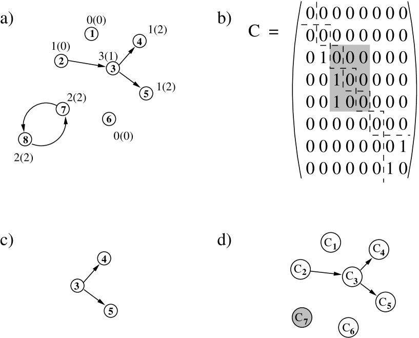
- Definition 2.2:
-
Adjacency matrix.
The adjacency matrix of a graph with nodes is an matrix, denoted , where if contains a directed link (arrow pointing from node to node ), and otherwise.
This convention differs from the usual one (Harary, 1969; Robinson and Foulds, 1980; Bollobás, 1998) where if and only if there is a link from node to node ; the transpose of the adjacency matrix defined above. This convention has been chosen because it is more convenient in the context of the dynamical system to be discussed in chapter 4. Figure 2.1b shows the adjacency matrix corresponding to the graph in Figure 2.1a. I will use the terms ‘graph’ and ‘adjacency matrix’ interchangeably: the phrase ‘a graph with adjacency matrix ’ will often be abbreviated to ‘a graph ’.
Undirected graphs are special cases of directed graphs whose adjacency matrices are symmetric (Harary, 1969; Robinson and Foulds, 1980). A single (undirected) link of an undirected graph between, say, nodes and , can be viewed as two directed links of a directed graph, one from to and the other from to . See Bollobás (1998) for many results concerning undirected graphs.
- Definition 2.3:
- Definition 2.4:
The graph in Figure 2.1c is thus an induced subgraph of the graph in Figure 2.1a (induced by ). For a subgraph it is often more convenient to label the nodes not by integers starting from 1, but by the same labels the corresponding nodes had in the parent graph. The adjacency matrix of an induced subgraph can be obtained by deleting all the rows and columns from the full adjacency matrix that correspond to the nodes outside the subgraph. The highlighted portion of the matrix in Figure 2.1b is the adjacency matrix of the induced subgraph in Figure 2.1c.
2.2 Degrees and dependency
2.2.1 Degree of a node and degree distribution of a graph
- Definition 2.5:
-
Degree, in-degree and out-degree.
The degree, or total degree, of a node is the total number of incoming plus outgoing links from that node, i.e., the degree of node is .
The in-degree of a node is the total number of incoming links to that node, i.e., the in-degree of node is .
The out-degree of a node is the total number of outgoing links from that node, i.e., the out-degree of node is (Harary, 1969; Bollobás, 1998).
The unbracketed numbers adjacent to each node in Figure 2.1a show the degree of that node.
2.2.2 Dependency and interdependency
- Definition 2.7:
-
Dependency.
The dependency, denoted , of a node is the total number of links in all paths that terminate at that node, each link counted only once (Jain and Krishna, 1999). - Definition 2.8:
-
Dependency distribution.
The dependency distribution of a graph, denoted , is the fraction of nodes with
dependency . - Definition 2.9:
-
Interdependency.
The interdependency of a graph is defined to be the average dependency:
(Jain and Krishna, 1999).
The bracketed numbers adjacent to each node in Figure 2.1a show the dependency of that node. The interdependency of the graph in Figure 2.1a is 9/8.
Because counts how many links ultimately ‘feed into’ the node , it is a measure of how ‘dependent’ node is on other nodes. Thus is a measure of how interdependent are the nodes in the graph. While the degree of a node is a ‘local’ measure as it depends only on the immediate connections of a node, the dependency is more ‘non-local’ in character because links far away from the node contribute to it.
2.3 Walks, paths and cycles
- Definition 2.10:
-
Walk, closed walk.
A walk of length (from node to node ) is an alternating sequence of nodes and links such that link points from node to node (i.e. ), points from to and so on. If the first and last nodes and of a walk are the same, it will be referred to as a closed walk
(Harary, 1969; Robinson and Foulds, 1980; Bollobás, 1998).
The existence of even one closed walk in the graph implies the existence of an infinite number of distinct walks in the graph. In the graph of Figure 2.1a, there are an infinite number of walks from node 7 to node 8 (e.g., , , ) but no walk from node 7 to node 2. An undirected graph trivially has closed walks if it has any undirected links at all.
If is the adjacency matrix of a graph then it is easy to see that equals the number of distinct walks of length from node to node . E.g., ; each term in the sum is unity if and only if there exists a link from to and from to , hence the sum counts the number of walks from to of length 2.
- Definition 2.11:
In a directed graph , I will say node ‘has access to’ node , or node ‘has access from’ node , if there is a path from node to node , i.e., for some (Rothblum, 1975). I refer to a node as being ‘downstream’ from a node if has access to , but does not have access to . Similarly is ‘upstream’ from if has access to , but does not have access to . Thus in Figure 2.1a, node 5 is downstream from node 2, or equivalently node 2 is upstream from node 5 because node 2 has access to 5 but not vice versa. Node 2 is neither upstream nor downstream from node 7 as neither have access to the other. Node 8 is also neither upstream nor downstream from 7 because each has access to the other along some directed path.
- Definition 2.12:
I will also use the term ‘cycle’ to refer to the subgraph consisting of the nodes and links that form the cycle. Thus any subgraph with nodes that contains exactly links and also contains a closed walk that covers all nodes is an -cycle. E.g., the subgraph induced by nodes 7 and 8 in Figure 2.1a is a 2-cycle. Clearly any graph that has a closed walk contains a cycle.
2.4 Connected components of a graph
Given a directed graph , its ‘associated undirected graph’ (or ‘symmetrized version’) can be obtained by adding additional links as follows: for every link in , add another link if the latter is not already in .
- Definition 2.13:
-
Strongly, weakly and unilaterally connected nodes.
Two nodes and of a directed graph will be said to be
(i) strongly connected if has access to and also has access to ,
(ii) unilaterally connected if either has access to , or has access to to ,
(iii) weakly connected if there exists a path between them in the associated
undirected graph ,
(iv) disconnected if none of the above is true (Harary, 1969; Robinson and Foulds, 1980).
It is evident that any strongly connected nodes are also unilaterally connected, and any unilaterally connected nodes are weakly connected, but the converse need not be true. A graph will be termed strongly, unilaterally, or weakly connected if all pairs of its nodes are, respectively, strongly, unilaterally or weakly connected. Any directed graph can be decomposed into strongly-, unilaterally- and weakly-connected components which are subgraphs induced by maximal sets of strongly, unilaterally and weakly connected nodes (Harary, 1969; Robinson and Foulds, 1980) (e.g., the graph of Figure 2.1a has five weakly connected components induced, respectively, by the nodes and ). By convention a single node is considered strongly-connected to itself even if there is no self-link (Harary, 1969; Robinson and Foulds, 1980). Therefore, if a graph contains a single node with no links the single node is also considered a (trivial) strong component of the graph.
2.5 Partitioning a graph into its strong components
The nodes of any graph can be grouped into a unique set of strong components as follows:
-
1.
Pick any node, say . Find all the nodes having access from . Denote this set by ; it may include itself. Similarly find all the nodes having access to . Denote this set by . Denote the subgraph induced by the set of nodes as . is one strongly connected component of the graph.
-
2.
Pick another node that is not in and repeat the procedure with that node to get another subgraph, . The sets of nodes comprising the two subgraphs will be disjoint.
-
3.
Repeat this process until all nodes have been placed in some , . Each is a strong component of the graph.
Irrespective of which nodes are picked and in which order, this procedure will produce for any graph a unique (upto labeling of the ) set of disjoint subgraphs, each of which is strongly connected, encompassing all the nodes of the graph (Harary, 1969; Robinson and Foulds, 1980). The graph in Figure 2.1a will decompose into 7 such subgraphs (comprising nodes and ).
One says there is a path from a strong component to another strong component if there is a path in from any node of to any node of . The terms ‘access’, ‘downstream’ and ‘upstream’ can thus be used unambiguously for the .
2.6 Condensation of a graph
- Definition 2.14:
-
Condensation of a graph.
Determine all the strong components of the graph as described above. Construct a new graph of nodes, one node for each , . The new graph has a directed link from to if, in the original graph, any node of has a link to any node of . This new graph is called the condensation of the graph
(Harary, 1969; Robinson and Foulds, 1980).
Figure 2.1d illustrates the condensation of Figure 2.1a. Clearly the condensed graph cannot have any closed walks. For if it were to have a closed walk then the subgraphs comprising the closed walk would together have formed a larger strong component in the first place. Therefore one can renumber the such that if , is never downstream from . Now one can renumber the nodes of the original graph such that nodes belonging to a given are labeled by contiguous node numbers, and whenever a pair of nodes and belong to different subgraphs and respectively, then implies . Such a renumbering is in general not unique, but with any such renumbering the adjacency matrix takes the following canonical form:
where indicates that the upper block triangular part of the matrix contains only zeroes while the lower block triangular part, , is not equal to zero in general. The matrix in Figure 2.1b is already in this canonical form; the dashed lines demarcate the portions that correspond to the .
2.7 Irreducible graphs and matrices
- Definition 2.15:
The simplest irreducible subgraph is a 1-cycle. In Figure 2.1a the subgraph induced by nodes 7 and 8 is irreducible, but the subgraph induced by nodes 2, 3, 4, and 5 is not irreducible as there is, for example, no path from node 5 to node 2.
- Definition 2.16:
-
Irreducible matrix.
A matrix is irreducible if for every ordered pair of nodes and there exists a positive integer such that (Seneta, 1973).
Thus, if a graph is irreducible then its adjacency matrix is also irreducible, and vice versa. Irreducible graphs are, by definition, strongly connected graphs. In fact all strongly connected graphs are irreducible, except the graph consisting of a single node with no self-link which is strongly connected (by definition) but not irreducible.
2.8 Perron-Frobenius eigenvectors (PFEs)
- Definition 2.17:
-
Eigenvector, eigenvalue.
A column vector is said to be a right eigenvector of an matrix with an eigenvalue if for each , . The eigenvalues of a matrix are roots of the characteristic equation of the matrix: , where is the identity matrix of the same dimensionality as and denotes the determinant of the matrix (Seneta, 1973).
A ‘left eigenvector’ is similarly defined to be a row vector such that for each , ; the left eigenvectors of are simply the transpose of the right eigenvectors of , the transpose of . In this thesis I will only use right eigenvectors and will therefore refer to them simply as eigenvectors. Note that the set of eigenvalues corresponding to all right eigenvectors is identical to the set of eigenvalues corresponding to the left eigenvectors. In general a matrix will have complex eigenvalues and eigenvectors, but an adjacency matrix of a graph has special properties, because it is a ‘non-negative’ matrix, i.e., it has no negative entries.
2.8.1 The Perron-Frobenius theorem
The Perron-Frobenius theorem for irreducible non-negative matrices
states (Seneta, 1973):
Suppose is an non-negative irreducible matrix.
Then there exists an eigenvalue such that:
a) is real, ;
b) with can be associated strictly positive left and right eigenvectors;
c) for any eigenvalue ;
d) the eigenvectors associated with are unique to constant multiples;
e) Let be any non-negative matrix. If
and is an eigenvalue of , then . Moreover,
implies ;
f) is a simple root of the characteristic equation of .
If the matrix is not irreducible a weaker form of the above theorem
holds. The Perron-Frobenius theorem for a general non-negative matrix
states (Seneta, 1973):
Suppose is an non-negative matrix. Then there exists
an eigenvalue such that:
a’) is real, ;
b’) with can be associated non-negative left and right eigenvectors;
c’) for any eigenvalue ;
e’) Let be any non-negative matrix. If
and is an eigenvalue of , then .
- Definition 2.18:
-
Perron-Frobenius eigenvalue.
For any graph , the eigenvalue of that is real and larger than or equal to all other eigenvalues in magnitude will be called the Perron-Frobenius eigenvalue of the graph and denoted by . The Perron-Frobenius theorem guarantees the existence of such an eigenvalue. - Definition 2.19:
-
Perron-Frobenius eigenvector (PFE).
For any graph , each eigenvector corresponding to consisting only of real and non-negative components will be referred to as Perron-Frobenius eigenvector (PFE). The Perron-Frobenius theorem guarantees the existence of at least one such eigenvector.
The Perron-Frobenius eigenvalue of the graph in Figure 2.1a is 1 and is a Perron-Frobenius eigenvector.
The presence or absence of closed walks in a graph can be determined from the Perron-Frobenius eigenvalue of its adjacency matrix:
- Proposition 2.1:
-
If a graph, ,
(i) has no closed walk then ,
(ii) has a closed walk then .
The proof of this and all subsequent propositions can be found in appendix A.
Note that cannot take values between zero and one because of the discreteness of the entries of , which are either zero or unity.
2.8.2 Basic subgraphs
In section 2.6 it was shown that the adjacency matrix of any graph can always be written in the following canonical form by an appropriate renumbering of the nodes:
From the above form of it follows that
Therefore the set of eigenvalues of is the union of the sets of eigenvalues of , which implies that . Thus, if a given graph has a Perron-Frobenius eigenvalue then it contains at least one strong component with Perron-Frobenius eigenvalue .
- Definition 2.20:
-
Basic subgraph.
Each strong components of with Perron-Frobenius eigenvalue equal to is referred to as a basic subgraph (Rothblum, 1975).
The shaded node in Figure 2.1d corresponds to the only basic subgraph of Figure 2.1a.
- Proposition 2.2:
-
If all the basic subgraphs of a graph are cycles then , and vice versa.

2.9 Random graphs
A random graph is an ensemble of graphs with each member of the ensemble having an associated probability (introduced by Erdős and Rényi, 1959). Two ensembles have been extensively studied. One, denoted , is the ensemble of graphs with vertices and links (and no self-links) with a uniform associated probability. The second is the ensemble of graphs, denoted , having vertices, with each possible link (except self-links) present with probability ; in other words the ensemble of all graphs with the probability associated with a graph being if it has links. These two ensembles have the same properties in the limit if (Bollobás, 1998, 2001). For the random graph the average number of links is , while the (total) degree distribution is binomial: (Bollobás, 1998, 2001). Figure 2.2 shows the dependency distribution of nodes of graphs picked from the ensemble with (the program rndgraph.cpp that is included in the attached CD, see appendix C, was used to generate the random graphs). The dependency averaged over all nodes was 0.33, and the standard deviation of dependency values was 0.76. The distribution appears to decline exponentially as a function of dependency value, but much slower than would be expected for a Poisson distribution with the same mean. See (Bollobás, 1998, 2001) for further results concerning random graphs.
Chapter 3 Autocatalytic Sets
This chapter discusses the notion of an ‘autocatalytic set’, which will play an important role in the dynamics of the model studied in this thesis. After first providing a graph-theoretic definition of an autocatalytic set, I discuss its relationship with the Perron-Frobenius eigenvectors of a graph. The rest of the chapter analyzes the structure of PFEs of different graphs, both ones which contains autocatalytic sets and ones which do not. The results derived here will prove useful in the analysis of the dynamical system discussed in chapter 4.
3.1 Autocatalytic sets (ACSs)
- Definition 3.1:
-
Autocatalytic set (ACS).
An autocatalytic set is a graph, each of whose nodes has at least one incoming link from a node belonging to the same graph (Jain and Krishna, 1998).
The concept of an ACS was introduced in the context of a set of catalytically interacting molecules where it was defined to be a set of molecular species that contains, within itself, a catalyst for each of its member species (Eigen, 1971; Kauffman, 1971; Rossler, 1971). Such a set of molecular species can collectively self-replicate under certain circumstances even if none of its component molecular species can individually self-replicate. This definition matches the one above if you imagine a node in a directed graph to represent a molecular species and a link from to to signify that is a catalyst for .
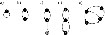
Figure 3.1 shows various ACSs. The simplest is a 1-cycle; Figure 3.1a. Figures 3.1a and 3.1b are graphs that are irreducible as well as cycles, 3.1c is an ACS that is not an irreducible graph and hence not a cycle, while 3.1d and 3.1e are irreducible graphs that are not cycles.
- Proposition 3.1:
-
(i) All cycles are irreducible graphs and all irreducible graphs are ACSs.
(ii) Not all ACSs are irreducible graphs and not all irreducible graphs are cycles.
3.2 Relationship between Perron-Frobenius eigenvectors and autocatalytic sets
The ACS is a useful graph-theoretic construct in part because of its connection with the PFE. Firstly, the Perron-Frobenius eigenvalue of a graph is an indicator of the existence of an ACS in the graph (Jain and Krishna, 1998, 1999):
- Proposition 3.2:
-
(i) An ACS must contain a closed walk. Consequently,
(ii) If a graph has no ACS then .
(iii) If a graph has an ACS then .
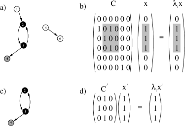
Let x be a PFE of a graph. Consider the set of all nodes for which is non-zero. I will call the subgraph induced by these nodes the ‘subgraph of the PFE x’. For example consider the graph in Figure 3.2a. For this graph . Figure 3.2b shows a PFE of the graph and how it satisfies the eigenvalue equation. For this PFE, nodes 1, 5 and 6 have . Removing these nodes produces the PFE subgraph shown in Figure 3.2c. If all the components of the PFE are non-zero then the subgraph of the PFE is the entire graph. One can show that (Jain and Krishna, 1998, 1999):
- Proposition 3.3:
-
If , then the subgraph of any PFE of is an ACS.
For the PFE of Figure 3.2b this is immediately verified by inspection. Note that this result relates an algebraic property of a graph, its PFE, to a topological structure, an ACS. Further, this result is not true if we considered irreducible graphs instead of ACSs.
- Proposition 3.4:
-
Let x be a PFE of a graph , and let denote the adjacency matrix of the subgraph of x. Let denote the Perron-Frobenius eigenvalue of . Then and must contain at least one of the basic subgraphs of .
Figure 3.2 illustrates this point. The adjacency matrix of the PFE subgraph, , is obtained by removing rows 1, 5, 6 and columns 1, 5, 6 from the original matrix. Figure 3.2d illustrates that the vector constructed by removing the zero components of the PFE is an eigenvector of with eigenvalue 1. contains one basic subgraph of – the one induced by the nodes 2 and 3.
3.3 Eigenvector profile theorem
I now present a series of propositions that describe some aspects of the ‘profile’ of possible PFEs of a graph, i.e., which components of the PFE are zero and which are non-zero. These propositions lead toward the eigenvector profile theorem which provides an algorithm for finding the profile of all the simple PFEs of a graph, and consequently the profile of the possible non-simple PFEs also. This theorem is completely general, applying to any given graph. After I had generated the proofs for the theorem and the propositions it depends upon, I found that these results had already been derived by Rothblum (1975) as part of a more general theorem concerning the profile of generalized eigenvectors of a non-negative matrix. The proofs provided in appendix A (Krishna and Jain, forthcoming) are, however, different from his; they make no use of the principle of mathematical induction, which Rothblum uses extensively.
For convenience I will often abbreviate statements like ‘there exists a PFE in which the components corresponding to the nodes in subgraph are non-zero/zero’ to ‘there exists a PFE in which the nodes in subgraph are non-zero/zero’.
- Proposition 3.5:
-
If a node is non-zero in a PFE then all nodes it has access to are non-zero in that PFE.
It follows that if any node of an irreducible subgraph is non-zero in a PFE then all the other nodes in that subgraph must be non-zero in that PFE. A situation where some nodes of an irreducible subgraph are non-zero and some are zero in the same PFE cannot happen.
- Proposition 3.6:
-
If a node is upstream from a basic subgraph then that node is zero in any PFE.
- Proposition 3.7:
-
If a node does not have access from a basic subgraph then it is zero in any PFE.
Propositions 3.6 and 3.7 describe which nodes will be zero in the PFEs, while proposition 3.4 and 3.5 describe which nodes will be non-zero – at least one of the basic subgraphs will be non-zero in every PFE along with all nodes it has access to. In other words the subgraph of any PFE consists of one or more of the basic subgraphs and those nodes that they have access to, i.e., the subgraph of any PFE is necessarily an ACS (recall proposition 3.3, this is an alternate proof of that proposition).
Propositions 3.4–3.7 can be used to prove the following theorem about the profile of PFEs of any graph:
- Theorem 3.1:
-
Eigenvector profile theorem
For any graph , determine all the basic subgraphs of . Denote them by . Determine which of these does not have any other downstream from it. Denote these by . Then:
(i) For each there exists a unique (upto constant multiples) PFE in which the nodes of and all nodes having access from them are non-zero and all other nodes are zero. It is evident that these PFEs are simple. Moreover these are the only simple PFEs of the graph .
(ii) Any PFE is a linear combination of these simple PFEs.
3.4 Core and periphery of a simple PFE
- Definition 3.3:
-
Core and periphery of a simple PFE.
If is the subgraph of a simple PFE, the basic subgraph contained in will be called the core of the simple PFE (or equivalently, the ‘core of ’), and denoted . The set of the remaining nodes and links of that are not in its core will together be said to constitute the periphery of the simple PFE (Jain and Krishna, 2003a).
For example, for the PFE in Figure 3.2b the core is the 2-cycle comprising nodes 2 and 3. In Figure 3.2 the core nodes are black and the periphery nodes grey. Note that the periphery is not a subgraph because it contains links not just between periphery nodes but also from nodes outside the periphery (like the link from node 3 to 4 in Figure 3.2c).
It follows from the Perron-Frobenius theorem for irreducible graphs that will necessarily increase if any link is added to the core. Similarly removing any link will decrease . Thus measures the multiplicity of internal pathways in the core. Figure 3.3 illustrates this point.

The core and periphery can be shown to have the following topological property (Jain and Krishna, 2003a):
- Proposition 3.8:
-
Every node in the core of a simple PFE has access to every other node of the PFE subgraph. No periphery node has access to any core node.
Thus starting from the core one can reach the periphery but not vice versa.
3.5 Core and periphery of a non-simple PFE
Because any PFE of a graph can be written as a linear combination of the simple PFEs (which, upto constant multiples, are unique for any graph), the definitions of core and periphery can be readily extended to any PFE as follows:
- Definition 3.4:
-
Core and periphery of a (non-simple) PFE.
The core of a PFE, denoted , is the union of the cores of those simple PFEs whose linear combination forms the given PFE. The rest of the nodes and links of the PFE subgraph constitute its periphery (Jain and Krishna, 2003a).
It follows from the above discussion that . When the core is a union of disjoint cycles then , and vice versa (recall proposition 2.2).
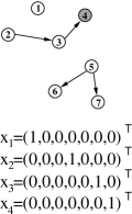
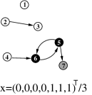
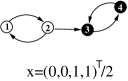
3.6 The profile of PFEs when there is no ACS
If , the graph has no ACS, then the profile of PFEs is as follows: for every node that has no outgoing links, there is a PFE with that node non-zero and all other nodes zero. For example the graph in Figure 3.4 has four (upto constant multiples) simple PFEs that are displayed in the same figure. This follows from theorem 3.1 because for a graph with each node is a basic subgraph. A general PFE is a linear combination of all such simple PFEs. Because there is no closed walk there is no core (or periphery) for any PFE of the graph. The core of all PFEs of such a graph may be defined to be the null set, .
3.7 The profile of PFEs when there is an ACS but only one basic subgraph
Now consider a graph that has , i.e., it contains an ACS, but has only one basic subgraph. In addition to the ACS it could possibly have various non-ACS structures such as chains, trees and isolated nodes. An example is the graph in Figure 3.5. For such a graph theorem 3.1 says that there is only one simple PFE in which the nodes in the basic subgraph and all nodes having access from it are non-zero, while the other nodes are zero (displayed in Figure 3.5). In particular the nodes in all non-ACS structures are zero in the (unique) PFE of the graph because they are don’t have access from the basic subgraph. The core nodes (nodes of the single basic subgraph) are black and the periphery nodes are grey in Figure 3.5. The white nodes are the nodes that are zero in the PFE of the graph.
3.8 The profile of PFEs when there is an ACS and many basic subgraphs
For any graph containing an ACS, i.e., one that has , there are possibly several simple PFEs as specified by theorem 3.1. However it follows from the theorem that in all the simple PFEs the nodes of non-ACS structures will be zero because they are not downstream from any basic subgraph.
While the nodes of non-ACS structures are guaranteed to be zero, it can also happen that the nodes of some basic subgraphs are zero in every PFE. Figure 3.6 illustrates such a case where the graph consists of one 2-cycle downstream from another. The Perron-Frobenius eigenvalue of this graph is , and each 2-cycle is a basic subgraph. From theorem 3.1 it follows that this graph has only one (simple) PFE (displayed in Figure 3.6) in which the upstream 2-cycle is zero.
Chapter 4 Population Dynamics
4.1 The population dynamics equation
In this chapter, I will analyze the attractors of the dynamical system described by the equation:
| (4.1) |
where lies on the simplex of normalized non-negative vectors in dimensions.
As discussed in section 1.7, the set of variables can be thought of as ‘living’ on the nodes of a graph whose adjacency matrix is . The links of the graph represent the interactions between the variables . It is useful to see how equation (4.1) arises in a chemical context.
Let denote a chemical (or molecular) species in a well-stirred chemical reactor. Molecules can react with one another in various ways; I focus on only one aspect of their interactions: catalysis. The catalytic interactions can be described by a directed graph with nodes. The nodes represent the species and the existence of a link from node to node means that species is a catalyst for the production of species . In terms of the adjacency matrix, of this graph, is set to unity if is a catalyst of and is set to zero otherwise. The operational meaning of catalysis is as follows:
Each species will have an associated non-negative population in the reactor that changes with time. Let species catalyze the ligation of reactants and to form the species , . Assuming that the rate of this catalyzed reaction is given by the Michaelis-Menten theory of enzyme catalysis, (Gutfreund, 1995), where are the reactant concentrations, and and are constants that characterize the reaction. If the Michaelis constant is very large this can be approximated as . Combining the rates of the spontaneous and catalyzed reactions and also putting in a dilution flux , the rate of growth of species is given by , where is the rate constant for the spontaneous reaction, and is the catalytic efficiency. Assuming the catalyzed reaction is much faster than the spontaneous reaction, and that the concentrations of the reactants are non-zero and fixed, the rate equation becomes , where is a constant. In general because species can have multiple catalysts, , with . I make the further idealization giving:
| (4.2) |
The relative population of species is by definition . As , . Taking the time derivative of and using (4.2) it is easy to see that is given by (4.1). Note that the term, present in (4.2), cancels out and is absent in (4.1).
Because we ultimately ignore the concentrations of the reactants we would get the same rate equations even if the reaction scheme were different, e.g., if only one reactant was required as in the reaction . Such dynamics might also be relevant in an economic context where the presence of one commodity increases the rate of production of another commodity.
Equation (4.1) has been used by Eigen et al. (1989) to describe the dynamics of the relative populations of self-replicating strings. Each node of represents one string. Two strings are connected by an undirected link if mutations of one string can produce the other; the strength of the link being a decreasing function of the number of mutations required. Eigen et al. have determined the attractor of equation (4.1) for the specific form this interpretation imposes on . Below, I analyze the attractors of equation (4.1) for an arbitrary graph , with no restrictions placed on its structure.
4.2 Attractors of the population dynamics equation
An important motivation for the choice of the population dynamics (4.1) is it’s analytical tractability. The following properties of the attractor can be derived (Jain and Krishna, 2003a; Krishna and Jain, forthcoming):
- Proposition 4.1:
-
For any graph ,
(i) Every eigenvector of that belongs to the simplex is a fixed point of equation (4.1), and vice versa.
(ii) Starting from any initial condition in the simplex , the trajectory converges to some fixed point (generically denoted X) in .
(iii) For generic initial conditions in , X is a Perron-Frobenius eigenvector (PFE) of .
(iv) If has a unique (upto constant multiples) PFE, it is the unique stable attractor of equation (4.1). -
(v) If has more than one linearly independent PFE, then X can depend upon the initial conditions. The set of allowed X is a linear combination of a subset of the PFEs. The interior of this set in may then be said to be the ‘attractor’ of (4.1), in the sense that for generic initial conditions all trajectories converge to a point in this set.
Statement (i) is easy to see: let be an eigenvector of , . Substituting this on the r.h.s. of (4.1), one gets zero. Conversely, if the r.h.s. of (4.1) is zero, , with .
Appendix A provides proof of the above propositions but they can be motivated by considering the underlying dynamics (4.2) from which (4.1) is derived. Because (4.1) is independent of , we can set in (4.2) without any loss of generality. With the general solution of (4.2), which is a linear system, can be schematically written as:
where and are viewed as column vectors. Suppose is a right eigenvector of with eigenvalue , denoted . Then
As this time dependence is merely a rescaling of the eigenvector, this is an alternative way of showing that is a fixed point of (4.1). If the eigenvectors of form a basis in , is a linear combination: . In that case, for large it is clear that the term with the largest value of will grow fastest, hence,
where is the eigenvalue of with the largest real part (which is the same as its Perron-Frobenius eigenvalue) and an associated eigenvector. Therefore, for generic initial conditions the trajectory of (4.1) will converge to , a PFE of . If the eigenvectors of do not form a basis in , the above result is still true (see appendix A).
Note that can be interpreted as the ‘population growth rate’ at large , because . In section 3.4, I had mentioned that measures a topological property of the graph, the multiplicity of internal pathways in the core of the graph. Thus, in the present model, has both a topological and dynamical significance, which relates two distinct properties of the system, one structural (multiplicity of pathways in the core of the graph), and the other dynamical (population growth rate). The higher the multiplicity of pathways in the core, the greater is the population growth rate of the dominant ACS.
4.3 Attractor profile theorem
While any eigenvector of is a fixed point it need not be stable. In other words, only for special initial conditions, forming a space of measure zero in , can X be some other eigenvector of , not a PFE. Henceforth, I ignore such special initial conditions. However, not all PFEs are attractors either. The following theorem indicates which subset of PFEs form the attractor set (Krishna and Jain, forthcoming):
- Theorem 4.1:
-
Attractor profile theorem
1) Determine all the strong components of the given graph . Denote these by .
2) Determine which of these are basic subgraphs. Denote them by .
3) Construct a graph, denoted , with nodes, representing the , and a link from node to node if there is a path from any node of to any node of that does not contain a node of any other basic subgraph.
4) Determine which of the are at the ends of the longest paths in the above graph . Denote these by .
For each there exists a unique (upto constant multiples) PFE that has only nodes of and all nodes having access from them non-zero, and all other nodes zero. The attractor set consists of all linear combinations of these PFEs that lie on the simplex .
4.4 The attractor for a graph with no ACS
For any graph that consists of only chains, trees and isolated nodes, i.e. any graph with , the theorem reduces to the following (Jain and Krishna, 1998, 1999):
- Proposition 4.2:
-
For any graph with , in the attractor only the nodes at the ends of the longest paths are non-zero. All other nodes are zero.
This follows from theorem 4.1 because for a graph with each node is a basic subgraph. Appendix A has an alternate proof based directly on the underlying dynamics. Figure 4.1 shows a graph that has . The white nodes are those that are zero in the attractor and the grey node is the only non-zero node in the attractor. This graph is the same as the one in Figure 3.4. Notice that of the four PFEs of the graph only one, , is the attractor.

4.5 The dominant ACS of a graph
For graphs with an ACS, i.e., with , recall that proposition 3.3 showed a close relationship between the PFEs of the graph and ACSs. A similar result holds for the attractor (Jain and Krishna, 1998, 1999):
- Proposition 4.3:
-
For any graph ,
(i) For every X belonging to the attractor set, the set of nodes for which is the same and is uniquely determined by . The subgraph formed by this set of nodes will be called the ‘subgraph of the attractor’ of (4.1) for the graph .
(ii) If , the subgraph of the attractor is an ACS.
- Definition 4.1:
The dominant ACS is independent of (generic) initial conditions and is the subgraph induced by the set of nodes belonging to all the and all nodes having access from them in . The following sections use theorem 4.1 to determine the structure of the dominant ACS of several different types of graphs.
4.6 Examples of the attractor for specific graphs
It is instructive to consider examples of graphs and see how the trajectory
converges to a PFE, and what the dominant ACS looks like in each case.
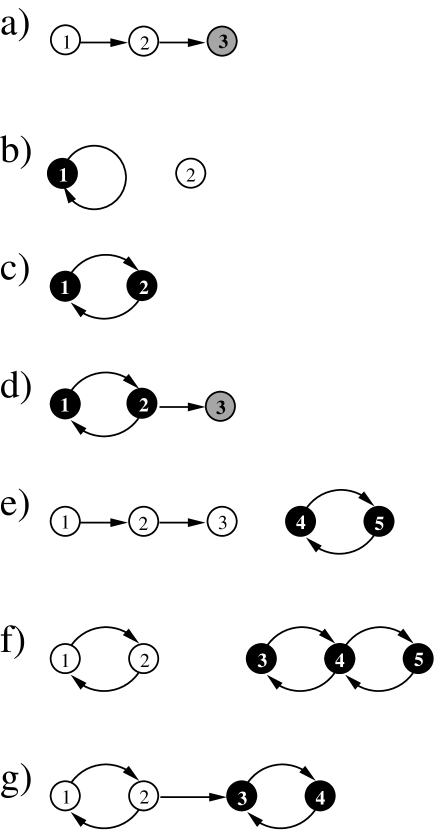
Example 1. A simple chain, Figure 4.2a:
The adjacency matrix of this graph has all eigenvalues zero; .
The unique PFE (upto constant multiples) of this graph is .
Because node 1 has no catalyst, its rate equation is (henceforth taking
) . Therefore , which
is a constant independent of . The rate equation for node 2 is
. Thus .
Similarly implies that .
At large , , , ;
hence dominates. Therefore,
is given by . Thus X equals
the unique PFE e, independent of initial conditions.
Example 2. A 1-cycle, Figure 4.2b:
This graph has two eigenvalues, , .
The unique PFE is . The rate equations are
, with the solutions .
At large node 1 dominates, hence .
The exponentially growing population of 1 is a consequence of the
fact that 1 is a self-replicator, as embodied in the equation .
Example 3. A 2-cycle, Figure 4.2c:
The corresponding adjacency matrix has eigenvalues .
The unique normalized PFE is . The population
dynamics equations are
The general solution to these is (note )
Therefore at large , ,
hence . Neither 1 nor 2
is individually a self-replicating node, but collectively they function
as a self-replicating entity.
Example 4. A 2-cycle with a periphery, Figure 4.2d:
This graph has and a unique normalized PFE .
The population equations for and and consequently
their general solutions are the same as Example 3, but now in addition
, yielding .
Again for large , grow as ,
hence . The dominant ACS
includes all the three nodes.
This example shows how a parasitic periphery (which does not feed
back into the core) is supported by an autocatalytic core. This is
also an example of the following general result: when a subgraph ,
with largest eigenvalue , is downstream
from another subgraph with largest eigenvalue ,
then the populations of the former also grow at the rate at which
the populations of are growing. Therefore if is non-zero
in the attractor, so is . In this example is the single
node 3 with and is the 2-cycle of nodes
1 and 2 with .
Example 5. A 2-cycle and a chain, Figure 4.2e:
The graph in Figure 4.2e combines the graphs
of Figures 4.2a and c. Following the analysis
of those two examples it is evident that for large , .
Because the populations of the 2-cycle are growing exponentially they
will eventually completely overshadow the populations of the chain
which are growing only as powers of . Therefore the attractor
will be which, it can be verified,
is a PFE of the graph (it is an eigenvector with eigenvalue 1). In
general when a graph consists of one or more ACSs and other nodes
that are not part of any ACS, the populations of the ACS nodes grow
exponentially while the populations of the latter nodes grow at best
as powers of . Hence ACSs always outperform non-ACS structures
in the population dynamics (see also Example 2).
Example 6. A 2-cycle and another irreducible graph
disconnected from it, Figure 4.2f:
One can ask, when there is more than one ACS in the graph which is
the dominant ACS? Figure 4.2f shows a graph containing
two strong components. The 2-cycle subgraph has a Perron-Frobenius
eigenvalue 1, while the other strong component has a Perron-Frobenius
eigenvalue . The unique PFE of the entire graph is
with eigenvalue . The population dynamics equations are
.
The first two equations are completely decoupled from the last three
and the solutions for and are the same as for Example
3. For the other irreducible graph the solution is (because )
Thus, the populations of nodes 3, 4 and 5 also grow exponentially
but at a faster rate, reflecting the higher Perron-Frobenius eigenvalue
of the subgraph comprising those nodes. Therefore, this structure
eventually overshadows the 2-cycle, and the attractor is .
The dominant ACS in this case is the irreducible subgraph formed by
nodes 3, 4 and 5. More generally, when a graph consists of several
disconnected ACSs with different individual , only
the ACSs whose are the largest (and equal to )
end up with non-zero relative populations in the attractor.
Example 7. A 2-cycle downstream from another 2-cycle,
Figure 4.2g:
What happens when the graph contains two ACSs whose individual
equals , and one of those ACSs is downstream of
another? In Figure 4.2g nodes 3 and 4 form a 2-cycle
that is downstream from another 2-cycle comprising nodes 1 and 2.
The unique PFE of this graph, with , is .
The population dynamics equations are .
Their general solution is:
It is clear that for large , .
While all four grow exponentially with the same rate ,
as and will overshadow
and . The attractor will be therefore be .
Here the dominant ACS is the 2-cycle of nodes 3 and 4. This result
generalizes to other kinds of ACSs: if one strong component is downstream
of another with the same Perron-Frobenius eigenvalue, the latter will
have zero relative population in the attractor.
The above examples displayed graphs with a unique PFE, and illustrated
proposition 4.1(iv). The stability of the attractor follows from the
fact that the constants , etc., in the above examples, that
can be traded for the initial conditions of the populations, do not
appear anywhere in the attractor X. Now I consider
examples where the PFE is not unique.
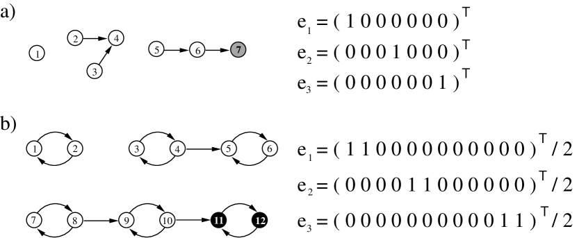
Example 8. Graph with and three
weakly connected components, Figure 4.3a:
This graph has three independent PFEs, displayed in Figure 4.3a.
The attractor is . This is an immediate
generalization of Example 1 above. Using the same argument as for
Example 1, we can see that if the longest path
ending at node is of length . Thus, the populations of nodes
1, 2, 3 and 5 are constant, those of 4 and 6 increase for
large , and of 7 as . Therefore, only nodes at the
ends of the longest paths will be non-zero in the attractor.
Example 9. Several weakly connected components
containing 2-cycles, Figure 4.3b:
Here again there are three PFEs, one for each weakly connected component.
The population of nodes in 2-cycles that are not downstream of other
2-cycles (nodes 1,2,3,4,7 and 8) will grow as . As in Example
7, Figure 4.2g, the nodes of 2-cycles that are
downstream of one 2-cycle (nodes 5, 6, 9 and 10) will grow as .
It can be verified that the populations of nodes in 2-cycles downstream
from two other 2-cycles (nodes 11 and 12) will grow as .
The pattern is clear: in the attractor only the 2-cycles at the ends
of the longest chains of 2-cycles will have non-zero relative populations.
Therefore, the attractor is .
4.7 Timescale for reaching the attractor
How long does it take the system to reach the attractor? This depends on the structure of the graph . For instance in Example 2, the attractor is approached as the population of node 1, , overwhelms the population . Because grows exponentially as , the attractor is reached on a timescale . (In general, when I say that ‘the timescale for the system to reach the attractor is ’, I mean that for , is ‘exponentially close’ to its final destination , i.e. for all , , with some finite .) In contrast, in Example 1, the attractor is approached as overwhelms and . Because in this case all the populations are growing as powers of , the timescale for reaching the attractor is infinite. When the populations of different nodes are growing at different rates, this timescale depends on the difference in growth rate between the fastest growing population and the next fastest growing population.
For graphs with like those in Example 1 and 8, all populations grow as powers of , hence the timescale for reaching the attractor is infinite.
For graphs that have but all the basic subgraphs are in different weakly connected components, such as Examples 2-6, the timescale for reaching the attractor is given by , where is the eigenvalue of with the next largest real part, compared to .
For graphs having with at least one basic subgraph downstream from another basic subgraph, the ratio of the fastest growing population to the next fastest growing one will always be a power of (as in Examples 7 and 9), therefore, the timescale for reaching the attractor is again infinite.
4.8 Core and periphery of a graph
As the dominant ACS is specified by a particular PFE, I will define the core of the dominant ACS to be the core of the corresponding PFE. If the PFE is simple, the core of the dominant ACS consists of just one basic subgraph. If the PFE is non-simple the core of the dominant ACS will be a union of more than one basic subgraph. The dominant ACS is uniquely determined by the graph. This motivates the definition of the core and periphery of a graph:
- Definition 4.2:
-
Core and periphery of a graph.
The core of a graph , denoted , is the core of the dominant ACS of , if an ACS exists in the graph. The periphery of is the periphery of the dominant ACS of . If no ACS exists in the graph, i.e., then (Jain and Krishna, 2003a).
In all cases . Henceforth all graphs will be depicted with the following colour scheme: black for core nodes, grey for periphery nodes (and for nodes with non-zero when there is no ACS), and white for nodes that are not in any of the PFE subgraphs.
4.9 Keystone nodes
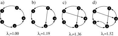
In ecology certain species are referred to as keystone species – those whose extinction or removal would seriously disturb the ecosystem (Paine, 1969; Jordán et al., 1999; Solé and Montoya, 2001). One might similarly look for the notion of a keystone node in a directed graph that captures some important organizational role played by a node. Consider the impact of the hypothetical removal of any node from a graph . One can, for example, study the structure of the core of the graph that would result if node (along with all its links) were removed from .
- Definition 4.3:
-
Core overlap.
Given any two graphs and whose nodes are labeled, the core overlap between them, denoted , is the number of common links in the cores of and , i.e., the number of ordered pairs for which and are both non-zero. If either or does not have a core, is defined to be zero (Jain and Krishna, 2002a). - Definition 4.4:
Thus a keystone node is one whose removal modifies the organizational structure of the graph (as represented by its core) drastically. In each of Figures 4.4a-d, for example, the core is the entire graph. In Figure 4.4a, all the nodes are keystone, because the removal of any one of them would leave the graph without an ACS (and hence without a core). In general when the core of a graph is a single -cycle, for any , all the core nodes are keystone. In Figure 4.4b, nodes 3, 4 and 5 are keystone but the other nodes are not, and in Figure 4.4c only nodes 4 and 5 are keystone. In Figure 4.4d, there are no keystone nodes. These examples show that the more internal pathways a core has (generally, this implies a higher value of ), the less likely it is to have keystone nodes, and hence the more robust its structure is to removal of nodes.
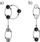
Figure 4.5 illustrates another type of graph structure that has a keystone node. The graph in Figure 4.5a consists of two strong components – a 2-cycle (nodes 4 and 5) downstream from an irreducible subgraph consisting of nodes 1, 2 and 3. The core of this graph is the latter irreducible subgraph. Figure 4.5b shows the graph that results if node 3 is removed with all its links. This consists of one 2-cycle downstream from another. Though both 2-cycles are basic subgraphs of the graph, as discussed in Example 7, Figure 4.2g, this graph has a unique (upto constant multiples) PFE, whose subgraph consists of the downstream cycle (nodes 4 and 5) only. Thus the 2-cycle 4-5 is the core of the graph in Figure 4.5b. Clearly . Therefore, node 3 in Figure 4.5a is a keystone node.
The above purely graph theoretic definition of a keystone node turns out to be useful in the dynamical system discussed in this and the following chapters. For other dynamical systems, alternate definitions of keystone might be more useful.
Chapter 5 Graph Dynamics
In this chapter, I present a model of an evolving network that is a specific instance of the framework described in section 1.7. The dynamical system described in the previous chapter is used for step 1 of the dynamics, and certain rules are chosen for steps 2 and 3 that aim to capture some features of the evolution of chemical networks on the prebiotic Earth.
5.1 Graph dynamics rules
The initial graph is constructed as follows: For every ordered pair with (where ), is independently chosen to be unity with a probability and zero with a probability . is set to zero for all . Thus the initial graph is a random graph, a member of the ensemble described in section 2.9. Each is chosen randomly, with uniform probability, in and all are rescaled so that .
-
Step 1.
With fixed, x is evolved according to (4.1) until it converges to a fixed point,
denoted X. -
Step 2.
The set of nodes with the least is determined, i.e, . A node, say node , is picked randomly from and is removed from the graph along with all its links.
-
Step 3.
A new node (also denoted ) is added to the graph. Links to and from to other nodes are assigned randomly according to the same rule, i.e, for every and are independently reassigned to unity with probability and zero with probability , irrespective of their earlier values, and is set to zero. All other matrix elements of remain unchanged. is set to a small constant , all other are perturbed by a small amount from their existing value , and all are rescaled so that .
This process, from step 1 onward, is iterated many times. Figure 5.1 depicts the graph dynamics schematically.

5.2 Features of the graph dynamics
5.2.1 Evolution in a prebiotic pool
These graph dynamics rules are motivated by the puzzle of how a complex chemical organization might have emerged from an initial ‘random soup’ of chemicals. As discussed in section 1.9, the rules model the imagined dynamics of an evolving chemical network such as might have existed in a pool on the prebiotic Earth. Several assumptions and idealizations underlie such a chemical interpretation of the model rules. Some of these have been mentioned in sections 1.9 and 4.1, however I will defer a more detailed discussion to section 9.3.
The model has two main sources of inspiration. One is the set of models studied by Farmer, Kauffman, Packard and others (Kauffman, 1983, 1993; Farmer et al., 1986; Bagley and Farmer, 1991; Bagley et al., 1991), and by Fontana (1991), and Fontana and Buss (1994) (see also Stadler et al., 1993; Dyson, 1985). Like these models, the present one employs an artificial chemistry of catalyzed reactions, albeit a much simpler one, in which populations of species evolve over time. To this I add the feature, inspired by the model of Bak and Sneppen (1993), that the ‘least fit species mutates’ with ‘fitness’ here being equated to the relative population. Unlike the Bak-Sneppen model, however, the ‘mutation’ of a species also changes its links to other species.
5.2.2 Coupling of population and graph dynamics: two timescales
As discussed in section 1.7, the coupling of the population dynamics and the graph dynamics is built into the framework of the model: the evolution of the depends on the graph in step 1, and the evolution of in turn depends on the through the choice of which node to remove in step 2. There are two timescales in the dynamics, a short timescale over which the graph is fixed while the evolve, and a longer timescale over which the graph is changed.
5.2.3 Absence of self-replicators
While in previous sections I have considered graphs with 1-cycles, the requirement in the present section forbids 1-cycles in the graph. The motivation is the following: 1-cycles represent self-replicating species (see previous section, Example 2). Such species, e.g., RNA molecules, are difficult to produce and maintain in a prebiotic scenario and it is possible that it requires a self-supporting molecular organization to be in place before an RNA world, for example, can take off (Joyce et al., 1987; Joyce, 1989). Thus, I wish to address the question: can one get molecular organizations that can collectively self-replicate without introducing self-replicating species ‘by hand’ into the system?
5.2.4 Selection and novelty
The rules for changing the graph implement selection and novelty, two important features of natural evolution. Selection is implemented by removing the node that is ‘performing the worst’, with ‘performance’ in this case being equated to a node’s relative population (step 2). Adding a new node introduces novelty into the system (step 3). Note that although the actual connections of a new node with other nodes are created randomly, the new node has the same average connectivity as the initial set of nodes. Thus, the new node is not biased in any way toward increasing the complexity of the chemical organization. Steps 2 and 3 implement the interaction of the system with the external environment. The phenomena to be described in the following sections are all consequences of the interplay between selection, novelty and the population dynamics.
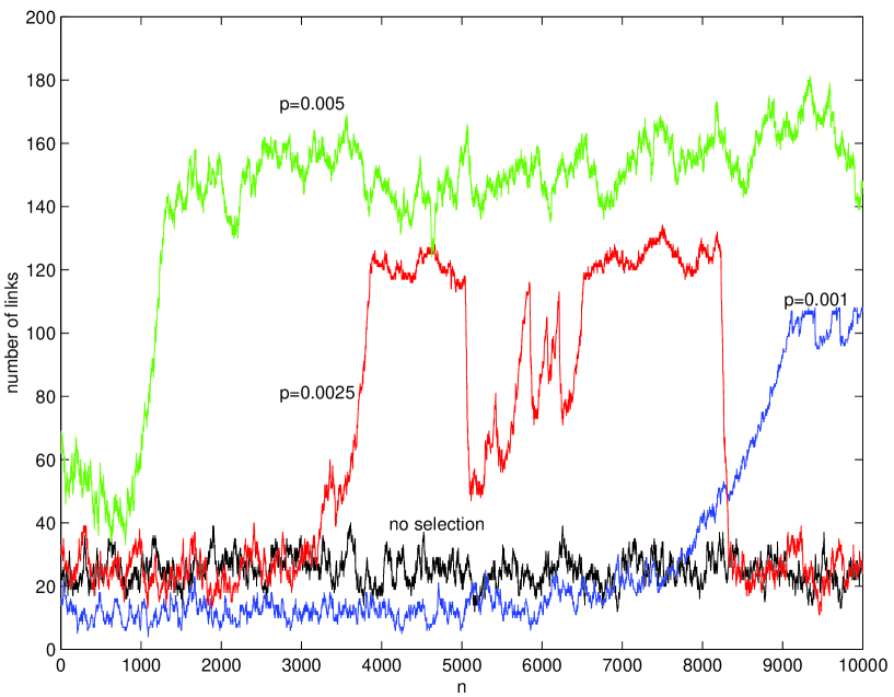
5.3 Implementation
Two programs are described in appendix B, and are included in the attached CD, that use different methods to implement the graph dynamics. The programs differ in the way the attractor is determined at each time step. The first program uses theorem 4.1. The second numerically integrates equation (4.1) to find its attractor. The programs are written in C++, with Matlab 5.2 being used to determine eigenvalues and eigenvectors where required.
5.4 Results of graph evolution
a)
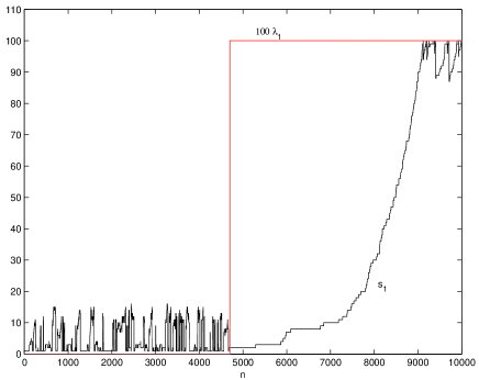
b)
c)

Figure 5.2 shows the total number of links in the graph versus time (, the number of graph updates). Three runs of the model described in the previous section, each with and different values of are exhibited. Also exhibited is a run where there was no selection (in which step 2 is modified: instead of picking one of the nodes of , any one of the nodes is picked randomly and removed from the graph along with all its links. The rest of the procedure remains the same). Figure 5.3 shows the time evolution of two more quantities for the same three runs with selection displayed in Figure 5.2. The quantities plotted are , the number of nodes with , and , the Perron-Frobenius eigenvalue of the graph. Figure 5.4 shows the evolution of another graph theoretic measure, the interdependency of the graph, , for the run of Figure 5.3b (the data files for these runs are included in the attached CD, see appendix C).
For all the displayed runs the size of the network has been taken to be . Computational constraints have prevented a detailed exploration of larger values of , though the few runs I have studied with values of upto 250 and have shown a similar behaviour. The values of the parameters and for the displayed runs were chosen to lie in the regime , and much of the analytical work described in later chapters, such as estimation of various timescales, assumes that . This range is the one of interest from the point of view of the origin of life problem because it is likely that the catalytic networks existing in prebiotic pools would have been quite sparse. However, it is worthwhile to extend the analysis and simulations to other parameter ranges, such as large or large values, and compare with the behaviour.
Coming back to the runs displayed in Figure 5.2, it is clear why the number of links fluctuates about its random graph value in the run without selection. This is because each graph update replaces a randomly chosen node with another that has on average the same connectivity and, therefore, the graph remains random like the starting graph. As soon as selection is added the behaviour becomes more interesting. Three regimes can be observed. First, the ‘random phase’ where the number of links fluctuates around , while and are small. Second, the ‘growth phase’ where , and show a clear rising tendency. Finally, the ‘organized phase’ where and hover (with large fluctuations) about a value much higher than the initial random graph value, and remains close to its maximum value (with some fluctuations). The time spent in each phase depends on and . I analyze the structure of the graph in the three phases in chapter 6.
Figure 5.5 shows for the same run as that of Figure 5.3b for a longer time, from to . In this long run one can see several sudden, large drops in : ‘catastrophes’ in which a large fraction of the nodes become extinct, i.e., the values of the nodes fell to zero. Some of the drops seem to take the system back into the random phase, others are followed by ‘recoveries’ in which rises back towards its maximum value . The recoveries are comparatively slower than the catastrophes, which in fact occur in a single time step. An analysis of crashes and recoveries is the subject of chapter 7.
It may be useful for the reader to trace the steps through one example run. Figure 5.6 shows snapshots of the graph at various times for the run shown in Figure 5.3b, which has . The initial random graph (, Figure 5.6a) has 31 links. 55 nodes are isolated with no incoming or outgoing links, and there are no cycles. In the attractor only node 13 is non-zero, all others are zero. Figures 5.6b-d show further snapshots of the graph in the random phase.
The first cycle comprising nodes 26 and 90 forms at (Figure 5.6e), and these nodes are the only non-zero ones in the attractor. This marks the beginning of the growth phase. At (Figure 5.6f) more nodes get attached to the cycle and their relative populations also become non-zero. By (Figure 5.6g) 28 nodes have added onto the 2-cycle. All these 30 nodes are non-zero in the attractor, while the other nodes are zero. At (Figure 5.6h) there is a sudden drop in as a new 2-cycle comprising nodes 41 and 98 is formed. This 2-cycle is downstream from the earlier 2-cycle, and for such a graph, as explained in section 4.6 (Example 7), only the downstream cycle will be non-zero. By (Figure 5.6i) the situation has not altered much, the old 2-cycle still survives by chance. But then node 38 gets removed, which breaks the path connecting the cycles. So at (Figure 5.6j) the graph consists of two disconnected 2-cycles. Both these cycles and all nodes having access from them are non-zero in the attractor. By (Figure 5.6k) several nodes have joined the 26-90 cycle. By chance none have joined the 41-98 cycle. At (Figure 5.6l) the 26-90 cycle gets strengthened by a second cycle. This subgraph now has a larger Perron-Frobenius eigenvalue and so the other cycle is zero in the attractor. After this the dominant ACS keeps accreting nodes until it spans the entire graph for the first time at (Figure 5.6m) signaling the start of the organized phase. At (Figure 5.6n) the core is at its largest. Most subsequent graph updates involve the removal of a node with no more drastic effect on the dominant ACS. This removed node will keep getting repeatedly replaced until it rejoins the dominant ACS. At (Figure 5.6o) the node 36 which is outside the ACS and therefore zero in the attractor, gets replaced and the new node rejoins the ACS resulting in the graph at (Figure 5.6p). Notice that node 36 forms a 2-cycle with node 74. Thus, this graph update has created a new irreducible subgraph in the periphery. At the moment this structure does not affect the dominant ACS because the core has a larger . However, a few hundred time steps later this 2-cycle plays a significant role.
![[Uncaptioned image]](/html/nlin/0403050/assets/x27.png)
![[Uncaptioned image]](/html/nlin/0403050/assets/x28.png)
![[Uncaptioned image]](/html/nlin/0403050/assets/x29.png)
![[Uncaptioned image]](/html/nlin/0403050/assets/x30.png)
![[Uncaptioned image]](/html/nlin/0403050/assets/x31.png)
![[Uncaptioned image]](/html/nlin/0403050/assets/x32.png)
![[Uncaptioned image]](/html/nlin/0403050/assets/x33.png)
![[Uncaptioned image]](/html/nlin/0403050/assets/x34.png)
![[Uncaptioned image]](/html/nlin/0403050/assets/x35.png)
![[Uncaptioned image]](/html/nlin/0403050/assets/x36.png)
![[Uncaptioned image]](/html/nlin/0403050/assets/x37.png)
![[Uncaptioned image]](/html/nlin/0403050/assets/x38.png)
![[Uncaptioned image]](/html/nlin/0403050/assets/x39.png)
![[Uncaptioned image]](/html/nlin/0403050/assets/x40.png)
![[Uncaptioned image]](/html/nlin/0403050/assets/x41.png)
![[Uncaptioned image]](/html/nlin/0403050/assets/x42.png)
![[Uncaptioned image]](/html/nlin/0403050/assets/x43.png)
![[Uncaptioned image]](/html/nlin/0403050/assets/x44.png)
![[Uncaptioned image]](/html/nlin/0403050/assets/x45.png)
![[Uncaptioned image]](/html/nlin/0403050/assets/x46.png)
![[Uncaptioned image]](/html/nlin/0403050/assets/x47.png)
![[Uncaptioned image]](/html/nlin/0403050/assets/x48.png)
![[Uncaptioned image]](/html/nlin/0403050/assets/x49.png)
![[Uncaptioned image]](/html/nlin/0403050/assets/x50.png)
y) n=8500 z) n=10000
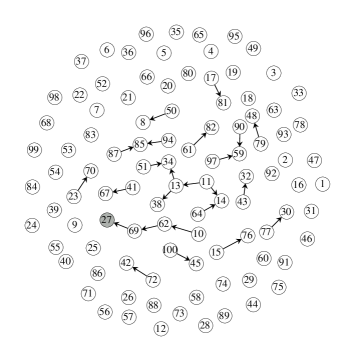
By (Figure 5.6q) the core has shrunk to 5 nodes. Node 85 gets removed which leaves the graph at (Figure 5.6r) with one 2-cycle (nodes 36 and 74) downstream from another (26 and 90). Only nodes 36, 74 and node 11 (downstream from 74) are non-zero in the new attractor. All other nodes have become extinct, triggering a drop in from 100 to 3. Over the next thousand time steps the dominant ACS rebuilds itself around the new core comprising nodes 36 and 74 (, Figure 5.6s). Then node 60 comes in, completing a cycle of 5 nodes that is downstream from the 36-74 cycle (, Figure 5.6t) and again there is a large drop in as 36, 74 and many nodes having access from them become extinct. At (Figure 5.6u), however, the 36-74 cycle is resurrected as the path connecting it to the 5-cycle is broken. It does not last for too long as the 5-cycle is strengthened by another cycle at (Figure 5.6v) and the 36-74 cycle again becomes extinct. This time it does not revive, as the dominant ACS builds around the strengthened 5-cycle. About two thousand time steps later, at (Figure 5.6w), the graph is again fully autocatalytic but is on the verge of a major collapse. The core is just a 3-cycle and node 54 gets removed, thus destroying the only cycle in the graph. The graph at (Figure 5.6x) is left without an ACS; the system is now once again in the random phase. Within a few hundred time steps all of the structure is destroyed and the graph at (Figure 5.6z) and (Figure 5.6z) are similar to the initial graph at (Figure 5.6a). At this point, I will stop following the run but eventually a new ACS arises, grows and spans the entire graph, then gets destroyed and another round starts (see Figure 5.5).
Chapter 6 Formation and Growth of Autocatalytic Sets
6.1 The random phase
For the run with displayed in Figure 5.3b, the initial random graph at contains no cycles, and hence no ACSs, and its Perron-Frobenius eigenvalue is . Figure 6.1 shows this initial graph.

For such a graph for all nodes that are at the ends of the longest paths of nodes, and for every other node (see section 4.4). In Figure 6.1, there are two paths of length 4, which are the longest paths in the graph. Both end at node 13, which is therefore the only non-zero node in the attractor for this graph. This node, then, is the only node protected from removal during the graph update. Node 13 has a high relative population but its supporting nodes do not have high relative populations. Inevitably within a few graph updates a supporting node will be removed from the graph. When that happens node 13 which presently has non-zero will no longer be at the end of the longest path and hence will get . In the run node 34 is replaced at the 8th time step. After that node 13 joins the set of nodes with least . Thus no structure is stable when there is no ACS. Eventually, all nodes are removed and replaced.
a)

b)

Figures 6.2 and 6.3 compare properties
of the graphs from the first random phase of the run (from
to , inclusive), with properties of the random graph ensemble,
, described in section 2.9. The average
number of links for the 2853 graphs in the random phase is 25.2, with
standard deviation 5.3. For the ensemble , with ,
the average number of links is . Figure 6.2
shows that the in and out degree distributions of graphs taken from
the random phase are close to the binomial distribution expected for
for smaller values of degree but depart from the binomial
for larger degrees. Figure 6.3 compares the dependency
distribution of the random phase with that of graphs taken
from the ensemble . Again, the distributions are similar
for smaller dependency values, and differ for higher values.
Although the properties of the random phase graphs do not exactly match the properties of graphs from the ensemble , the main point about the graph dynamics holds nevertheless: In the random phase no graph structure is stable for very long and eventually all nodes are removed and replaced.
Note that the initial random graph is likely to contain no cycles when is small (). If larger values of are chosen, it becomes more likely that the initial graph will contain a cycle. If it does, there is no random phase; the system is then in the growth phase, discussed below, right from the initial time step.

6.2 The growth phase
At some graph update an ACS is formed by pure chance. The probability of this happening can be closely approximated by the probability of a 2-cycle (the simplest ACS with 1-cycles being disallowed) forming by chance, which is (= the probability that in the row and column corresponding to the replaced node in , any matrix element and its transpose are both assigned unity). Thus, the ‘average time of appearance’ of an ACS is , and the distribution of times of appearance is . This approximation is better for small . In the run displayed in Figure 5.3b, a 2-cycle between nodes 26 and 90 formed at . This is a graph that consists of a 2-cycle and several other chains and trees. For such a graph, I have shown in Example 3 in section 4.6 that the attractor has non-zero for nodes 26 and 90 and zero for all other nodes. The dominant ACS consists of nodes 26 and 90. Therefore these nodes cannot be picked for removal at the graph update and, hence, a graph update cannot destroy the nodes and links of the dominant ACS. The autocatalytic property is guaranteed to be preserved until the dominant ACS spans the whole graph. In fact, an even stronger statement can be made (Jain and Krishna, 1998, 1999):
- Proposition 6.1:
-
is a non-decreasing function of as long as .
When a new node is added to the graph at a graph update, one of three things will happen:
-
1.
The new node will not have any links from the dominant ACS and will not form a new ACS. In this case the dominant ACS will remain unchanged, the new node will have zero relative population and will be part of . For small this is the most likely possibility.
-
2.
The new node gets an incoming link from the dominant ACS and hence becomes a part of it. In this case the dominant ACS grows to include the new node. For small , this is less likely than the first possibility, but such events do happen and in fact are the ones responsible for the growth of the dominant ACS.
-
3.
The new node forms another ACS. This new ACS competes with the existing dominant ACS. Whether it now becomes dominant, overshadowing the previous dominant ACS or it gets overshadowed, or both ACSs coexist depends on the Perron-Frobenius eigenvalues of their respective subgraphs and how they are connected. Again, for small , this is a rare event compared with possibilities 1 and 2.
Typically the dominant ACS keeps growing by accreting new nodes, usually one at a time, until the entire graph is an ACS. At this point the growth phase stops and the organized phase begins.
6.2.1 Timescale for growth of the dominant ACS
Assuming that possibility 3 above is rare enough to neglect, and that the dominant ACS grows by adding a single node at a time, one can estimate the time required for it to span the entire graph. Let the dominant ACS consist of nodes at time . The probability that the new node gets an incoming link from the dominant ACS and hence joins it is . Thus in graph updates, the dominant ACS will grow, on average, by nodes. Therefore , where , is the time of appearance of the first ACS and is the size of the first ACS (=2 for the run shown in Figure 5.3b). Thus is expected to grow exponentially with a characteristic timescale . The time taken from the appearance of the ACS to its spanning is . This analytical result is confirmed by simulations (see Figure 6.4). In the displayed run, after the first ACS (a 2-cycle) is formed at , it takes 1026 time steps, until for the dominant ACS to span the entire graph. This explains how an autocatalytic network structure and the positive feedback processes inherent in it can bootstrap themselves into existence from a small seed. The small seed, in turn, is guaranteed to appear on a certain timescale ( in the present model) just by random processes.

6.3 Fully autocatalytic graphs
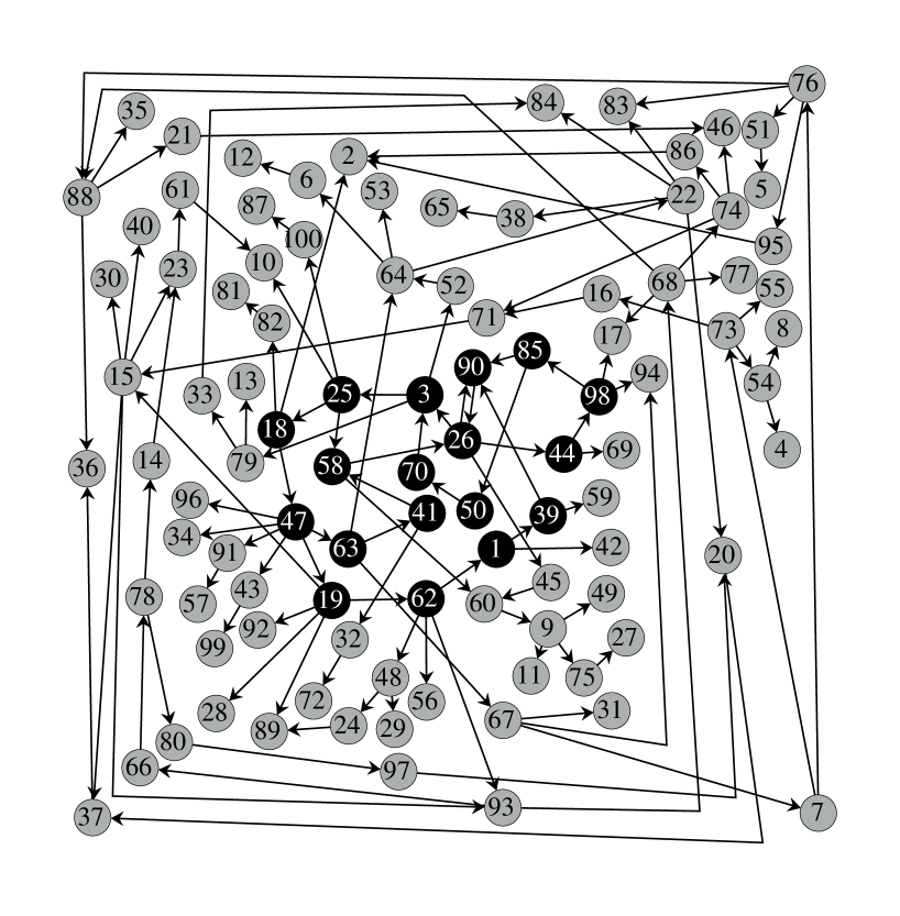
The growth phase continues until the dominant ACS spans the entire graph. In the displayed run this happened at . Figure 6.5 shows the graph at this time – it is a fully autocatalytic graph, all nodes are part of the dominant ACS.
6.3.1 Probability of a random graph being fully autocatalytic
A fully autocatalytic graph such as this is a highly improbable structure
for a random graph. Consider a graph of nodes and let the probability
of a positive link existing between any pair of nodes (except self-links)
be . Such a graph has on average incoming
or outgoing positive links per node. For the entire graph to be an
ACS, each node must have at least one incoming link, i.e. each row
of the matrix must contain at least one positive element. Hence
the probability, , for the entire graph to be an ACS is
| probability that every row has at least one positive entry | ||
| [probability that a row has at least one positive entry | ||
| probability that every entry of a row is zero | ||
| . |
Note from Figure 5.2 that at spanning the number of links is 124, i.e., . Thus the average degree at spanning is . I have found this to be true in all the runs I have done where was or less.
For large and , , where is positive, and . Thus, a fully autocatalytic graph is exponentially unlikely to form if it were being assembled randomly (or picked at random from the random graph ensemble ). In the present model nodes are being added completely randomly but the underlying population dynamics and the selection imposed at each graph update result in the inevitable arrival of an ACS (in, on average, time steps) and its inevitable growth into a fully autocatalytic graph in (on average) an additional time steps.
For the displayed run if we take we get . Even if we take to be the average degree of the graph at , i.e., we get ; one would expect such a fully autocatalytic graph to take time steps to form if it were being assembled randomly, in contrast to the 3880 time steps it actually took in this run.
As mentioned in section 1.9, one of the puzzles of the origin of life is: how could a highly structured chemical network form in such a short time after the oceans condensed on the Earth? In this model, a highly non-random structure, a fully autocatalytic set, inevitably forms. Further, the time taken for it to form is extremely short, growing only as a logarithm of the size of the network. This model, therefore, suggests a mechanism – the growth of ACSs by the accretion of nodes around a small initial ACS – by which highly structured chemical networks (that are exponentially unlikely to form by chance) can form in a very short time. This mechanism, or its analogue in a more realistic chemical model, might explain the emergence of a structured chemical organization on the prebiotic Earth. This is discussed further in section 9.2.
6.3.2 Clustering coefficient
In several runs with (totaling 1.55 million iterations) 160659 graphs were fully autocatalytic. The mean clustering coefficient of these 160659 graphs was 0.025, with standard deviation 0.016, which is comparable to the clustering coefficient for random graphs with the same connectivity (, see below). The graph in Figure 6.5, in fact, has a clustering coefficient of zero: none of the neighbours of any node are connected to each other, as can be verified from the figure. Thus, the fully autocatalytic graphs produced in these runs do not have a small-world structure.
6.3.3 Degree and dependency distributions
The in-degree and out-degree distributions of the nodes of all the 160659 fully autocatalytic graphs produced in these runs are shown in Figure 6.6. The mean in-degree for nodes of these graphs was 1.27, and the standard deviation was 0.50. The mean out-degree was 1.27, with standard deviation 1.75. The distributions are compared with the binomial distribution (as expected for random graphs from the ensemble ; ) and the shifted binomial (as would be expected for a random autocatalytic graph). The in-distribution is quite similar in functional form to the shifted binomial for small in-degrees but departs from it for higher values. In contrast, the out-distribution falls off much more slowly, though it is not scale-free either because it is not a straight line in a log-log plot (Figure 6.7). However, as , the allowed values for the degree of a node cover a range of only two decades. If a portion of the out-degree distribution is a power-law then it is more likely to show up for graphs with higher , where the degree distributions would span more decades. For such networks, with larger , whether the fully autocatalytic graphs produced are scale-free or not is an open question.
The dependency distribution of the fully autocatalytic graphs produced in the runs (Figure 6.8) has a substantially larger mean than the distribution for graphs of the random phase (compare with Figure 6.3). This is consistent with the growth of interdependency observed in Figure 5.4. Further, as evident from Figure 6.8, the dependency distribution is also clearly different from, and much narrower than, the distribution for random graphs with a comparable connectivity . The mean dependency of nodes of the fully autocatalytic graphs (30.93, with standard deviation 14.71) is slightly larger than the mean dependency for random graphs, , with (23.70, with standard deviation 30.82), but the maximum dependency observed for the fully autocatalytic graphs (100) is smaller than the maximum for the random graphs (163). In all the fully autocatalytic graphs, the minimum dependency was two, and the dependency distribution is small for small values of dependency. In contrast, the dependency distribution for the random graphs is maximum at zero dependency.
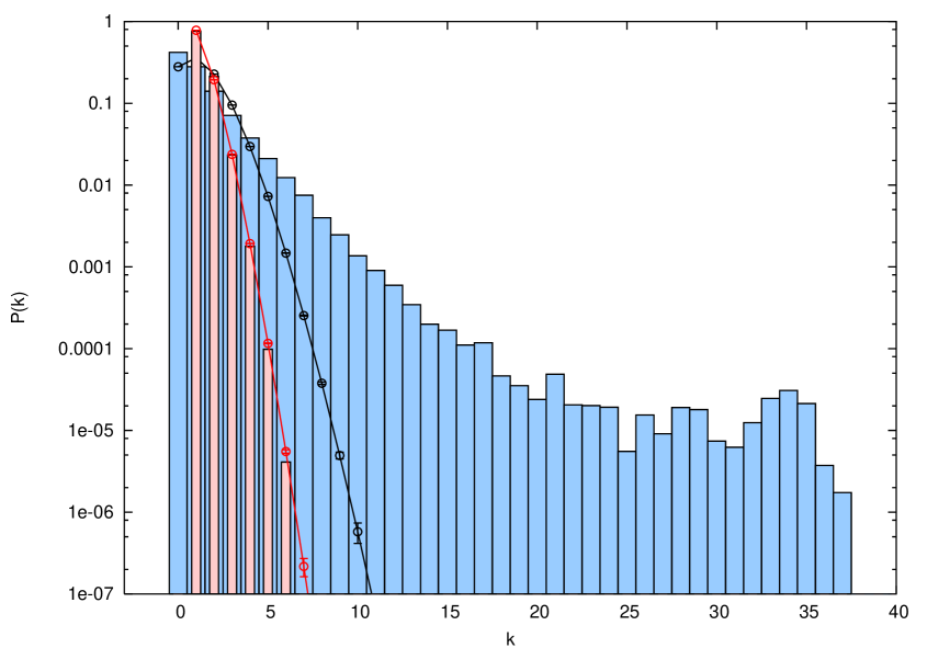


Chapter 7 Destruction of Autocatalytic Sets
7.1 Catastrophes and recoveries in the organized and growth phases
Once an ACS spans the entire graph the effective dynamics again changes although the microscopic dynamical rules are unchanged. At spanning, for the first time since the formation of the initial ACS, a node of the dominant ACS will be picked for removal. This is because at spanning all nodes belong to the dominant ACS and have non-zero relative populations; one node nevertheless has to be picked for removal. Most of the time the removal of the node with the least will result in minimal damage to the ACS. The rest of the ACS will remain with non-zero relative populations, and the new node will repeatedly be removed and replaced until it once again joins the ACS. Thus will fluctuate between and most of the time. However, once in a while, the node that is removed happens to be playing a crucial role in the graph structure despite its low relative population. Then its removal can trigger large changes in the structure and catastrophic drops in and . Alternatively, it can sometimes happen that the new node added can trigger a catastrophe because of the new graph structure it creates.
In Figure 5.5, which shows for the same run as that in Figure 5.3b but for a much longer time, one can observe several of the large and sudden drops in that will be discussed in this chapter. These ‘catastrophes’ in the organized and growth phases are followed by ‘recoveries’, in which rises on a certain timescale. Figure 7.1 shows the probability distribution of changes in the number of nodes with ; . The asymmetry between rises and drops as well as fat tails in the distribution are evident. For low the probability of large drops is an order of magnitude greater than intermediate size drops (also see Figure 5.3).
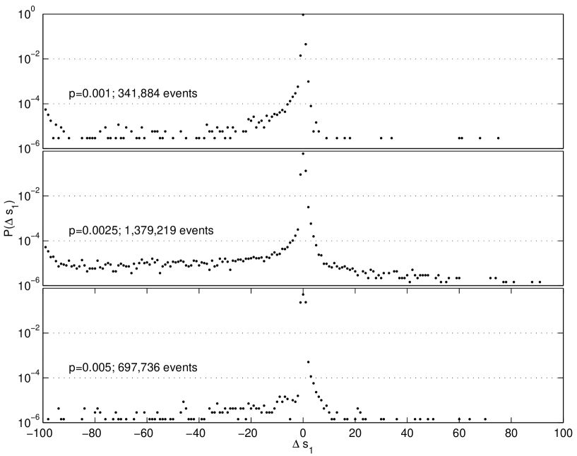
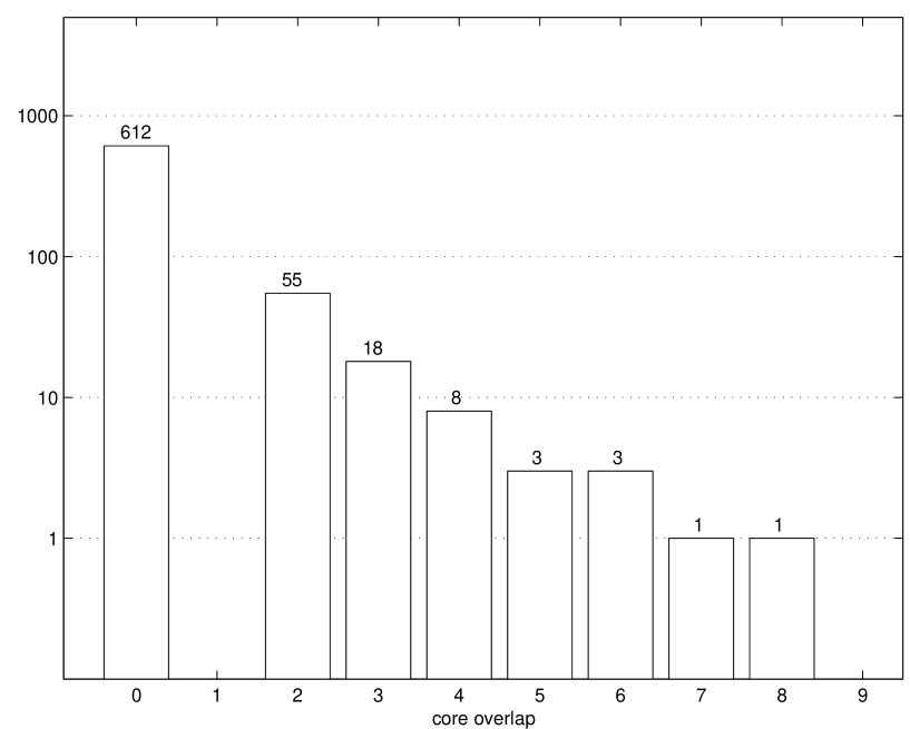
7.2 Crashes and core-shifts
- Definition 7.1:
A crash is an event in which a significant fraction (arbitrarily chosen as 50%) of the nodes become extinct. In several runs with totaling 1.55 million iterations there were 701 crashes. The first task is to see if these large drops in are correlated to specific changes in the structure of the graph.
- Definition 7.2:
Figure 7.2 shows a histogram of core overlaps for these 701 crashes. 612 of these have zero core overlap, i.e., they are core-shifts. (If one looks at only those events in which more than 90% of the nodes went extinct, i.e., , then one finds 235 such events in the same runs, out of which 226 are core-shifts.) Of the remaining 89 crashes 10 were events in which the core remained unchanged and 79 were events in which the core was affected but some overlap remained between the new and old cores. Most of the crashes happen when there is a core-shift – a drastic change in the structure of the dominant ACS.
In the 612 core-shifts, the average number of incoming plus outgoing links is 2.27 for all nodes in the graph, 2.25 for the node that is removed and 1.25 for the new node. Thus the nodes whose removal or addition causes the crash are not excessively rich in links. ‘Nondescript’ nodes such as these cause system wide crashes because of their critical location in a small core (the average core size at the 612 core-shifts is 6.3 nodes). Core-shifts in which the ACS is completely destroyed typically cause the largest damage (of 612 core-shifts these are 136 in number, with ). The remaining 476 core-shifts in which an ACS exists after the core-shift have . The former constitute an increasing fraction of the crashes at smaller values, causing the upturn in at large negative for small (Figure 7.1).
7.3 Addition and deletion of nodes from a graph
In order to understand what is happening during the crashes and subsequent recoveries I begin by examining the possible changes that an addition or a deletion of a node can make to the core of the dominant ACS.
7.3.1 Deletion of a node: keystone nodes
We have already seen how the deletion of a node can change the core – recall the discussion of keystone nodes in section 4.9: the removal of a keystone node results in a core-shift, i.e., a zero overlap between the cores of the dominant ACS before and after the removal. In an actual run a keystone node can only be removed if it happens to be one of the nodes with the least . However, the core nodes are often ‘protected’ by having higher . The reason for this is:
X is an eigenvector of with eigenvalue . Therefore, when it follows that for nodes of the dominant ACS, . If node of the dominant ACS has only one incoming link (from the node , say) then ; is ‘attenuated’ with respect to by a factor . The periphery of an ACS is a tree-like structure emanating from the core, and for small most periphery nodes have a single incoming link. For instance, the graph in Figure 7.3, whose , has a chain of nodes . The farther down such a chain a periphery node is, the lower is its because of the cumulative attenuation. For such an ACS the ‘leaves’ of the periphery tree (such as node 6) will have the least while core nodes will have larger .
However, when there is no attenuation. At the core must be a cycle or a set of disjoint cycles (proposition 2.2), hence each core node has only one incoming link within the dominant ACS. All core nodes have the same value of . As one moves out toward the periphery, implies there is no attenuation, hence each node in the periphery that receives a single link from one of the core nodes will also have the same . Some periphery nodes may have higher if they have more than one incoming link from the core. Iterating this argument as one moves further outward from the core, it is clear that at the core is not protected and in fact will always belong to (the set of nodes with the least ) if the dominant ACS spans the graph. We have already seen in section 4.9 that when and the core is a single cycle every core node is a keystone node. Thus, when the organization is fragile and susceptible to core-shifts caused by the removal of a keystone node.
![[Uncaptioned image]](/html/nlin/0403050/assets/x65.png)
7.3.2 Addition of a node: innovations
I now turn to the effects of the addition of a node. The removal and subsequent addition of a new node in a graph update creates a new graph that is likely to have a different attractor from the previous graph. In the new attractor the new node, denoted , may become extinct, i.e., may be zero, or it may survive, i.e., is non-zero. If the new node becomes extinct then it remains in the set and there is no change to the dominant ACS. So I will focus on events in which the new node survives in the new attractor.
- Definition 7.3:
I will also use the term ‘innovation’ to refer to the new structures created – the new node and the new links brought in by the graph update event. Figure 7.4 shows a graph-theoretic classification of innovations in terms of a hierarchy. The innovations that have the least impact on the relative populations of the nodes and the evolution of the graph on a short timescale (of a few graph updates) are ones that do not affect the core of the dominant ACS, if it exists. Such innovations are of three types (see boxes 1–3 in Figure 7.4):
1. Random phase innovations. These are innovations that occur in the random phase when no ACS exists in the graph, and they do not create any new ACSs. These innovations are typically short lived and have little short or long term impact on the structure of the graph. In the displayed run the first random phase innovation appeared at (node 25 in Figure 5.6c).
2. Incremental innovations. These are innovations that occur in the growth and organized phases, which add new nodes to the periphery of the dominant ACS without creating any new irreducible subgraph. See Figure 5.6f, , for the first incremental innovation of the displayed run. In the short term these innovations only affect the periphery and are responsible for the growth of the dominant ACS. In a longer term they can also affect the core as chains of nodes from the periphery join the core of the dominant ACS.
3. Dormant innovations. These are innovations that occur in the growth and organized phases, which create new irreducible subgraphs in the periphery of the dominant ACS (e.g. the innovation at , Figure 5.6p, that created the 2-cycle 36-74 in the periphery). These innovations too affect only the periphery in the short term. But they have the potential to cause core-shifts later if the right conditions occur (see section 7.4.3).
Innovations that do immediately affect the core of the existing dominant ACS are always ones which create a new irreducible subgraph. They are also of three types (boxes 4–6 in Figure 7.4):
4. Core enhancing innovations. These innovations result in the expansion of the existing core by the addition of new links and nodes from the periphery or outside the dominant ACS. They result in an increase of of the graph. The innovation at (Figure 5.6l) is an example.
5. Core-shifting innovations. These are innovations that cause an immediate core-shift often accompanied by the extinction of a large number of nodes. The innovation at (Figure 5.6t) is an example (also see section 7.4.2).
6. Creation of the first ACS. This is an innovation that creates the first ACS in a graph which till then had none. In the displayed run, the first ACS was created at (Figure 5.6d,e). The innovation moves the system from the random phase to the growth phase.
- Definition 7.4:
-
Core transforming innovation.
An innovations of type 4, 5 or 6 which immediately affects the core of the dominant ACS will be called a core transforming innovation (Jain and Krishna, 2003a).
The following proposition makes precise the conditions under which a core transforming innovation can occur (Jain and Krishna, 2003a). Let denote the graph of nodes just after the node is removed from . will stand for the core of .
- Proposition 7.1:
-
Let denote the maximal new irreducible subgraph that includes the new node at time step . will become the new core of the graph, replacing the old core , whenever either of the following conditions are true:
(a) or,
(b) and is downstream of .
Such a core transforming innovation will fall into category 4 above if . However, if and are disjoint, we get a core-shift and the innovation is of type 5 if is non-empty or type 6 otherwise.
7.4 Classification of core-shifts
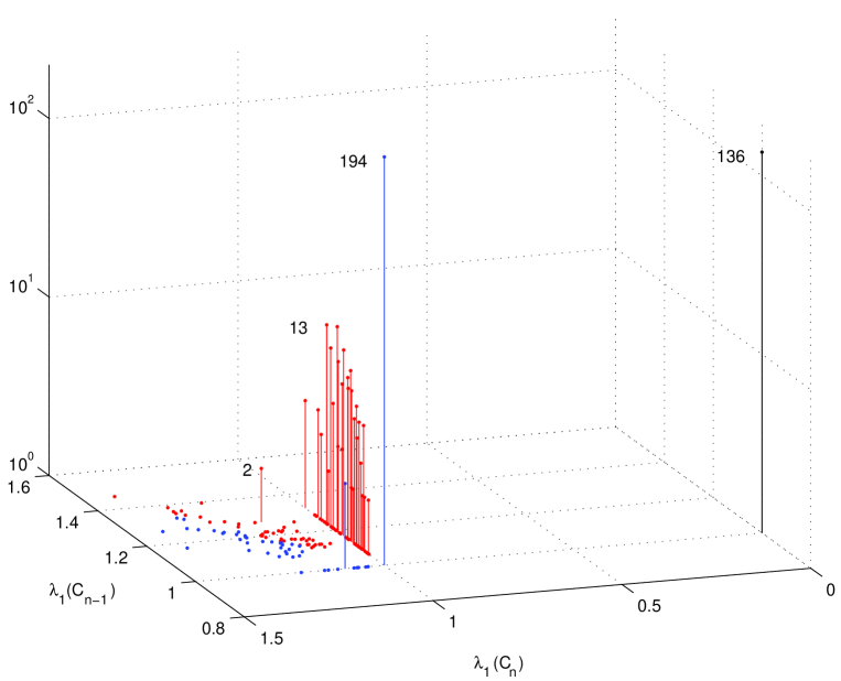
Using the insights from the above discussion of the effects of deletion or addition of a node, one can classify the different mechanisms that cause core-shifts. Figure 7.5 differentiates the 612 core-shifts observed among the 701 crashes. They fall into three categories: (i) complete crashes ( events), (ii) takeovers by core-transforming innovations ( events), and (iii) takeovers by dormant innovations ( events).
7.4.1 Complete crashes
n=8232 n=8233
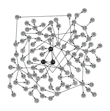
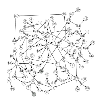
A complete crash is an event in which an ACS exists before but not after the graph update. Such an event takes the system into the random phase. A complete crash can occur when a keystone node is removed from the graph. For example, in the run displayed in Figure 5.3b and 5.6, at (see Figure 7.6), the graph had and its core was the simple 3-cycle of nodes 20, 50 and 54. As we have seen above, when the core is a single cycle every core node is a keystone node and is also in the set of nodes with the least . Node 54 was removed, thus disrupting the 3-cycle. The resulting graph, at , had no ACS and dropped to zero. As discussed earlier, graphs with are the ones that are most susceptible to complete crashes. This can be seen in Figure 7.5: every complete crash occurred from a graph with .
7.4.2 Takeovers by core transforming innovations
n=6061 n=6062
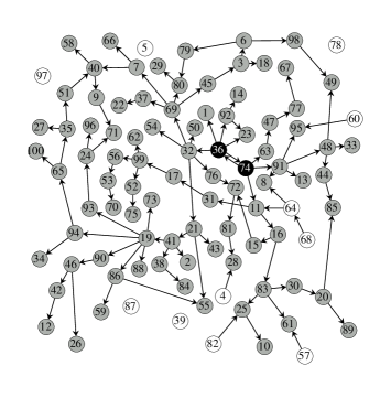
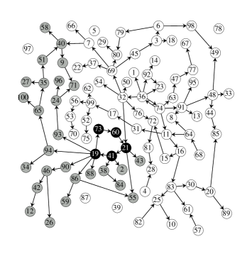
n=5041 n=5042
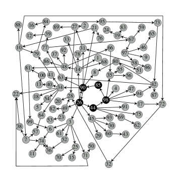
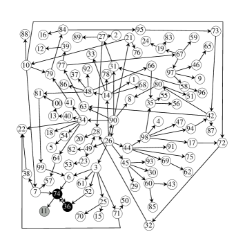
An example of a takeover by a core-transforming innovation is given in Figure 7.7, taken from the example run of Figure 5.3b. At the core was a single cycle comprising nodes and . Node was replaced at creating a 5-cycle comprising nodes and , downstream from the old core. The graph at has one cycle feeding into a second cycle that is downstream from it. We have already seen in section 4.6 (see the discussion of Example 4) that for such a graph only the downstream cycle is non-zero and the upstream cycle and all nodes dependent on it become extinct. Thus, the new cycle becomes the new core and the old core becomes extinct resulting in a core-shift. This is an example of condition (b) for a core-transforming innovation. For all such events in Figure 7.5, because happened not to be a core node of . Thus, these core-shifts satisfy in Figure 7.5.
7.4.3 Takeovers by dormant innovations
Dormant innovations, which create an irreducible structure in the periphery of the dominant ACS that does not affect its core at that time, were discussed in section 7.3.2. An example is the 2-cycle comprising nodes 36 and 74 formed at . At a later time such a dormant innovation can result in a core-shift if the old core gets sufficiently weakened.
In this case the core has become weakened by , when it has (Figure 7.8). The structure of the graph at this time is very similar to the graph in Figure 4.5a. Just as node 3 in Figure 4.5a was a keystone node, here nodes 44, 85, and 98 are keystone nodes because removing any of them results in a graph like Figure 4.5b, consisting of two 2-cycles, one downstream from the other.
Indeed, at , node is replaced and the resulting graph at has a 2-cycle ( and ) downstream from another cycle ( and ). Thus, at , nodes and form the new core with only one other downstream node, , being non-zero. All other nodes become extinct resulting in a drop in by . A dormant innovation can takeover as the new core only following the removal of a keystone node that weakens the old core. In such an event the new core necessarily has a lower (but non-zero) than the old core, i.e., (see Figure 7.5).
Note that is a keystone node and the graph is susceptible to a core-shift because of the innovation that created the cycle 36-74 earlier. If the cycle between and were absent would not be a keystone node because its removal would still leave part of the core intact (nodes and ).
7.5 Timescale of crashes
I will denote by the time elapsed between successive crashes, not counting the time spent in the recovery from the previous crash (i.e., the time from the previous crash to the first subsequent spanning of the graph by the dominant ACS). Figure 7.9a shows the distribution of values for the 701 crashes, discussed above, observed in runs with . The average and the standard deviation of values is for these 701 crashes. Figure 7.9b shows the distribution of values. The distribution and the value must be taken with caution because the distribution appears to be a very broad one (the standard deviation of values is larger than ) and 701 instances may not be enough to specify it accurately.
a)

b)

a)

b)

7.6 Recoveries
After a complete crash the system is back in the random phase. In graph updates each node is removed and replaced by a randomly connected node, resulting in a graph as random as the initial graph. Then the process starts again, with a new ACS being formed after an average of time steps and then growing to span the entire graph after, on average, time steps, where is the size of the initial ACS that forms in this round (typically for small ).
After other catastrophes, an ACS always survives. In that case the system is in the growth phase and immediately begins to recover, with growing exponentially on a timescale . Note that these recoveries happen because of innovations (mainly of type 2 and 4, and some of type 3).
7.7 Structure of the graph just before a crash

The in-degree and out-degree distributions of the nodes of the 701 graphs just before each crash are shown in Figure 7.10. The distributions are compared with the distributions for all fully autocatalytic graphs produced in the same runs. Both the distributions fall off faster than the distributions for all fully autocatalytic graphs.
Another interesting difference between the graphs just before a crash and all fully autocatalytic graphs lies in their dependency distributions: The dependency distribution of the graphs before crashes (Figure 7.11) is bimodal, in contrast to the distribution for all fully autocatalytic graphs which is unimodal and has a larger mean.

Figure 7.12 compares the distribution of Perron-Frobenius eigenvalues for the 701 graphs with the distribution for all the fully autocatalytic graphs. For the graphs just before each of the 701 crashes the mean Perron-Frobenius eigenvalue is 1.07, with standard deviation 0.10 – clearly lower than the mean for the fully autocatalytic graphs, which is 1.43, with standard deviation 0.20. The three mechanisms that cause core-shifts, discussed previously, are all more likely to happen with graphs whose cores are cycles. Therefore, it is not surprising that the graph just before a crash tends to have a Perron-Frobenius value close to unity.
Chapter 8 Robustness of the ACS Growth Mechanism
8.1 Variants of the model
In this chapter, I examine the effect of various modifications to the model rules on the formation and growth of ACSs. These modifications relax several of the simplifications that have been made, which depart from realism but make the model simpler to analyze:
-
1.
take values 0 and 1 only; all catalysts have the same catalytic efficiency.
-
2.
take positive values only; negative links – inhibitors – are not present in the model.
-
3.
Diagonal elements are zero; no self-replicators are allowed.
-
4.
The node with the least is removed at each graph update; extremal selection.
-
5.
If several nodes have the same least only one is removed.
-
6.
The total number of nodes is fixed; the rate of node removals and node additions is exactly the same.
-
7.
The population dynamics is linear in the variables.
I consider the following variants of the model, that relax these simplifications:
-
1.
Variable link strengths. , when non-zero, are allowed to take any value in the interval . This relaxes simplification (1).
-
2.
Negative links. , when non-zero, are allowed to take negative values also. This relaxes simplifications (1) and (2).
-
3.
Self-replicators. The diagonal elements, , are allowed to take non-zero values. This relaxes simplification (3).
-
4.
Non-extremal selection. Simplification (4) is relaxed in three variants, in which the dynamics is made non-extremal in different ways:
-
(a)
A fixed fraction of the nodes with the least are replaced at each graph update.
-
(b)
A single node is picked for removal, with a probability proportional to , at each graph update. When some nodes have then one of them is picked randomly.
-
(c)
The selection depends on a parameter, denoted . At each graph update, the node to be removed is selected from the set of nodes with least with a probability , or randomly from all nodes with a probability .
-
(a)
-
5.
Variable number of nodes. A fixed threshold is chosen and at each graph update all nodes with are removed and one new node is brought in. This relaxes simplifications (5) and (6).
-
6.
Different population dynamics. An equation for in which the first term is quadratic in the relative population variables is used instead of equation (4.1). This relaxes simplification (7).
8.2 Variable link strengths
The first modification I examine is allowing to take values in the interval , instead of just the values 0 or 1. The initial graph is constructed as follows: for each ordered pair with , is non-zero with probability and with probability . If non-zero, the value of is randomly picked from the interval with uniform probability. As before is set to zero for all to disallow self-replicators. Step 3 of the graph dynamics – addition of a new node – is similarly modified. Apart from these alterations the model remains unchanged.
a)

b)

Figure 8.1 shows a run with these modifications in the rules. The same behaviour is seen. There is a ‘random phase’ where there is no ACS and the graph remains random. The chance formation of an ACS on an average timescale triggers the ‘growth phase’ in which the number of non-zero nodes grows exponentially with a characteristic timescale , until the ACS spans the entire graph.
This is expected because most of the analytical results hold, with minor modifications, for this variant too. The Perron-Frobenius theorem holds for the adjacency matrices of the graphs produced because they are still non-negative. The only significant modification in the analytical results is that now can take values between 0 and 1 also. For example, consider the 2-cycle shown in Figure 8.2. The strengths of the two links are and , any real numbers in the interval . For such a graph .

Thus, the condition is changed to in all propositions that contain it. Proposition 2.1(ii) is modified to read: If a graph has a closed walk then . Proposition 3.2(iii) is similarly modified: If a graph has an ACS then .
The only difference this makes to the dynamics of the system is that in this variant it is much less likely for two disjoint ACSs with the same value to exist in some graph. In the original model two or more ACSs, typically cycles, often coexisted in runs with small (see Figures 5.6j,u). With variable link strengths even if two disjoint cycles form the chance of their having exactly the same value is negligible.
8.3 Negative links: emergence of cooperation
Now I generalize the model to include inhibitory reactions (where a species can decrease the rate of production of another species) along with variable link strengths. I implement this by modifying the way links are assigned in the initial random graph and to the new node at each graph update: if is chosen to be non-zero then it is assigned randomly a value in the interval if or if (self-replicators continue to be disallowed but self-inhibitors are possible). With negative links the populations can become negative. To prevent this a cutoff must be put on when becomes zero:
| (8.1) |
For simplicity I retain the form of (4.2) although a more realistic chemical interpretation would require to be proportional to for inhibitory reactions.

The cutoff in the population dynamics makes it a nonlinear equation. As a result now the attractor need not be only a fixed point. For most graphs I have encountered in simulations the attractor of (8.2) has been a fixed point. In less than 0.2% cases the attractor has been a limit cycle where the relative populations of the nodes oscillate. I have not observed any other types of attractors. The simplest type of graph having a limit cycle attractor consists of 3 nodes and is displayed in Figure 8.3. For this graph each oscillates around a mean value of with a frequency . The amplitude of oscillation depends on the initial condition but is always equal for the 3 nodes. If the amplitudes are smaller than then none of the hit zero and the cutoff in (8.2) plays no role in the oscillations. However if arbitrarily random small changes are made to the interaction strengths of the graph the oscillations of the start hitting zero and the cutoff comes into play. In general the cutoff seems to play an important role in limit cycle attractors. It is only in some special cases and for particular initial conditions that the relative populations of nodes oscillate without hitting zero. Numerical observations indicate that the property of having a limit cycle attractor is structurally stable, i.e., a limit cycle attractor remains if sufficiently small changes are made to the interaction strengths of a given graph having a limit cycle attractor.
a)
b)
The theorems used to analyze the attractors of the original model depended on the matrix being non-negative and hence no longer hold for the system with negative links. However numerical simulations of the system show behaviour very similar to the original system (Jain and Krishna, 2001) despite the slight bias toward negative links (because self-inhibitors are allowed but not self-replicators). Figure 8.4 shows the results of a run with and . The number of nodes with , , after the addition of a new node, the number of positive (), , and negative links (), , are displayed. Similar to the original model, the curves have three distinct regions. Initially is small; most of the nodes have zero . and also do not vary much from their initial value () and remain approximately equal. In the second region and show a sharp increase while decreases. In the third region the growth of and stops and almost all nodes have non-zero in contrast to the initial period. The number of positive links have increased to several times their initial value while the number of negative links has declined to about . I have observed the same qualitative behaviour in several runs with values ranging from to and .
Again the explanation for the above behaviour lies in the formation and growth of autocatalytic sets. The definition of an ACS has to be slightly modified: an ACS is a subgraph, each of whose nodes has at least one incoming positive link from a node belonging to the same subgraph. Proposition 3(i) also has to be similarly modified: An ACS must contain a cycle of positive links.
Upto , there is no ACS; the graph has no cycles of positive links. For such graphs, I find that for most nodes except a few at which the longest paths of positive links terminate, with intermediate nodes not having incoming negative links. This is a numerical observation that is similar to proposition 4.2. Thus most nodes have . Nodes with will also join the set of nodes with least if one of their supporting nodes is picked for removal from the system. Hence, all nodes are susceptible to be removed sooner or later; the graph remains as random as the initial graph and so , and hover around their initial values. The dramatic increases in and are triggered by the chance formation of an ACS at . In this system too an ACS will inevitably form by pure chance sooner or later. The ‘time of appearance’ of an ACS can again be approximated by the time of formation of a 2-cycle of positive links. As one wants the 2-cycle to contain positive links only, in the previous formula for has to be replaced by . Thus for and ) and .
From to (when first reaches ), I again find that the set of nodes with is an ACS; the ‘dominant ACS’. This is also a numerical observation. The proof of proposition 4.3 no longer holds but the system nevertheless shows identical behaviour in this respect to the system with only positive links. Hence, as long as the dominant ACS does not span the entire graph, i.e. , there are nodes outside it with which form the set . Therefore, none of the nodes in the dominant ACS can be removed in the next graph update.

All the processes that can happen in the original model when a new node is brought in (numbered 1, 2 and 3 in section 6.2) happen in this system with the same effects. The only new possibility to which the presence of negative links leads is when the new node joins the dominant ACS and some of the other nodes in the dominant ACS receive negative links from it. Then those nodes may become extinct causing to decrease. An example of this is shown in Figure 8.5. A new node, 3, is added to a previously existing 2-cycle. It gets a positive incoming link from node 2 and a negative outgoing link to node 1. This negative link destroys the ACS. In the attractor only node 3 is non-zero while node 1 and 2 have . Node 3 is like a destructive parasite that feeds on the the host ACS (nodes 1 and 2) to increase its own relative population, in the process destroying the host. The negative link is essential for the destructive property of such parasites; in the system with only positive links only benign parasites are possible that do not harm the ACS upon which they are feeding. This example also shows that propositions 4.3 and 6.1 are no longer true; the set of nodes with need not be an ACS even if an ACS exists in the graph and can decrease while . However, destructive parasites occur rarely and do not reverse the trend of increasing – in the displayed run they formed times at and , and in each case only resulted in decreasing by . Because the dominant ACS grows by adding positive links to the existing dominant ACS, the number of positive links increases as the ACS grows. On the other hand nodes receiving negative links often have , hence negative links get eliminated when these nodes are removed.
One can calculate the growth rate of the dominant ACS in exactly the same way as for the system with positive links because destructive parasites appear rarely. The only difference is that must be replaced by because that is the probability for the added node to get a positive link to/from any other node. Thus once an ACS forms, locally averaged in time grows exponentially with a characteristic timescale . This is confirmed by numerical simulations (Figure 8.6).
This variant of the model, apart from being an important test of the robustness of the ACS mechanism, also allows one to address questions concerning the emergence of ‘cooperation’ because negative links can arise in the network. The negative links in the network can be considered ‘destructive’ links as they cause one species to decrease the population growth rate of another. In contrast, the positive links in the network can be considered ‘cooperative’ links. The increase of the ratio of positive to negative links, from its initial value of unity to value more than an order of magnitude larger in Figure 8.4, is evidence of the emergence of cooperation during the run.
8.4 Self-replicators

In the original model, and all the variants discussed so far, self-replicators, i.e., self-links from a node to itself, are disallowed. As discussed in section 5.2.3, this was done to see whether structured chemical networks can arise even in the (forced) absence of individual self-replicators. As shown in chapter 6, structured networks do indeed form. The question that now arises is: Will allowing self-links interfere with the formation and growth of other ACSs? In fact, it does not, as evidenced by Figure 8.7, which shows a run with negative links in which self-replicators were allowed, i.e., for the initial graph and for the new node (when non-zero) was chosen randomly from the interval . The probability for a self-replicator to form in a graph update event is . The probability for a 2-cycle to form is . These are comparable when . Thus for small enough , self-replicators do form, and often trigger the growth phase, but their role in the network dynamics is similar to that of any other ACS. Self-replicators have a Perron-Frobenius eigenvalue and are, therefore, no more robust than cycles. ACSs with larger Perron-Frobenius eigenvalues out-compete self-replicators.
8.5 Non-extremal selection
The rule for removing a node can be made non-extremal in various ways. Instead of removing a single node with the least one can remove more than one node or remove nodes with higher also. However, even when removing nodes which do not have the least it is reasonable to allow some bias in favour of nodes with a higher . I consider the following possibilities:
-
1.
A fixed fraction of the nodes with the least are replaced at each graph update.
-
2.
A single node is picked for removal, with a probability proportional to , at each graph update. When some nodes have then one of them is picked randomly.
-
3.
The selection depends on a parameter, denoted . At each graph update, the node to be removed is selected from the set of nodes with least with a probability , or randomly from all nodes with a probability .
Figure 8.8a shows a run with with 2 nodes removed at each graph update; case 1 with . Figure 8.8b shows a similar run with 10 nodes removed at each graph update. Figure 8.9 shows a run with for case 2. In these three runs the behaviour is similar to the earlier models. An ACS forms by chance and grows until most of the graph is autocatalytic. In these cases the nodes comprising the dominant ACS are protected from removal until the size of the ACS becomes close to . Only after the ACS has become more than for Figure 8.8a, more than for Figure 8.8b, or has reached for Figure 8.9 do nodes of the dominant ACS start getting removed in the graph updates.
Case 3 is designed to interpolate between the extremal selection of the original model () and the completely random run where there is no selection (, see black curve in Figure 5.2). Figure 8.10 displays what happens for different values of . The basic mechanism of an ACS forming and growing remains but as is decreased the ACS becomes increasingly short lived and susceptible to destruction. Suppose the ACS has indispensable nodes, any of whose removal would destroy the ACS. Then the probability that an indispensable node will be removed is . Hence, there exists a timescale over which an ACS will get destroyed due to non-extremality. On the other hand for small ACSs get destroyed even with extremal dynamics over a timescale . does change with time but by choosing sufficiently close to 1, one can make . In that case the behaviour would be the same as in the case of extremal dynamics. This is confirmed by the run in Figure 8.10c, where an ACS forms and grows until it spans the entire graph. After spanning it does not get destroyed for a substantial period of time.
a)
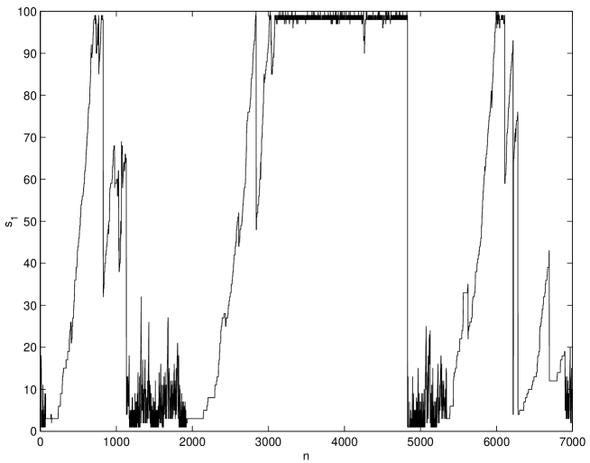
b)
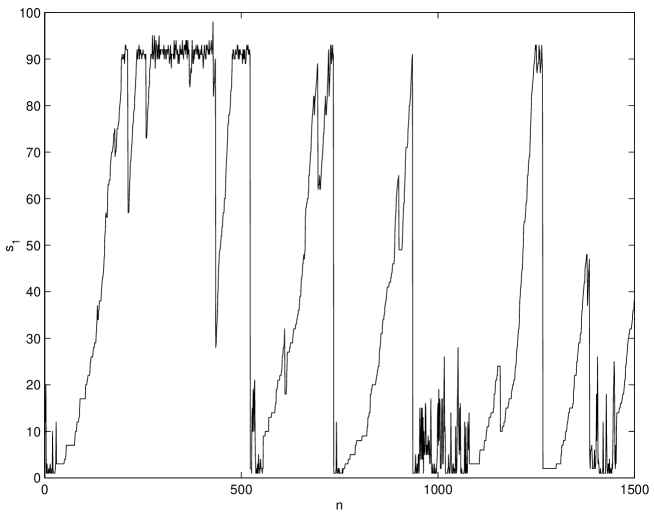
These non-extremal runs seem to indicate that the ACS mechanism is stable to the introduction of non-extremality. In an ACS, organizationally important nodes, such as the core nodes, tend to have high relative populations and, therefore, these nodes are protected if there is a selective bias that favours removing nodes with less relative population. When the mechanism for choosing a node for removal is not based on the relative population of nodes, as (partially) in case 3, this protection is lost and the ACS is not as robust a structure.
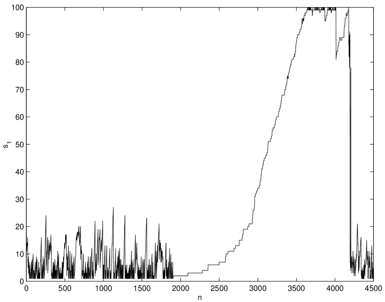
a)
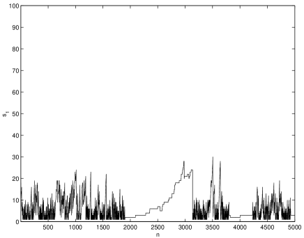
b)
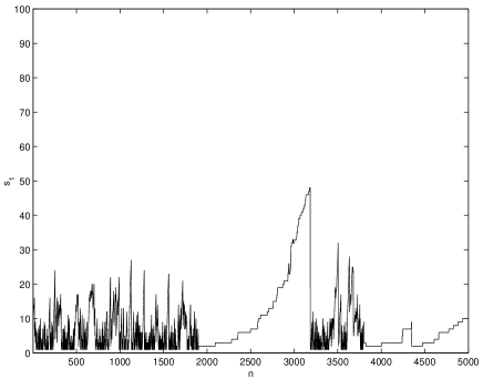
c)
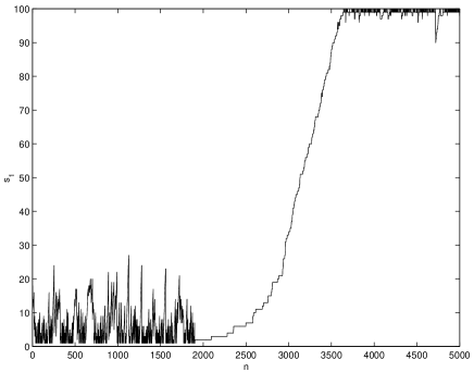
8.6 Variable number of nodes
Another idealization in the original model is that at each time step exactly one node is removed and one node is introduced leaving the total number of nodes constant. A variant in which the number of nodes is not constant is the following: at each time step, all nodes with below a fixed threshold, , are removed (more than one node can get deleted and the number of nodes is not constant). The rest of the procedure remains the same; one new node is added, the population dynamics is allowed to run its course with the new graph, and this is iterated many times. Notice that it is also possible for none of the nodes to be removed in a particular time step if they all have relative populations above . This is not possible in the original model.
a)
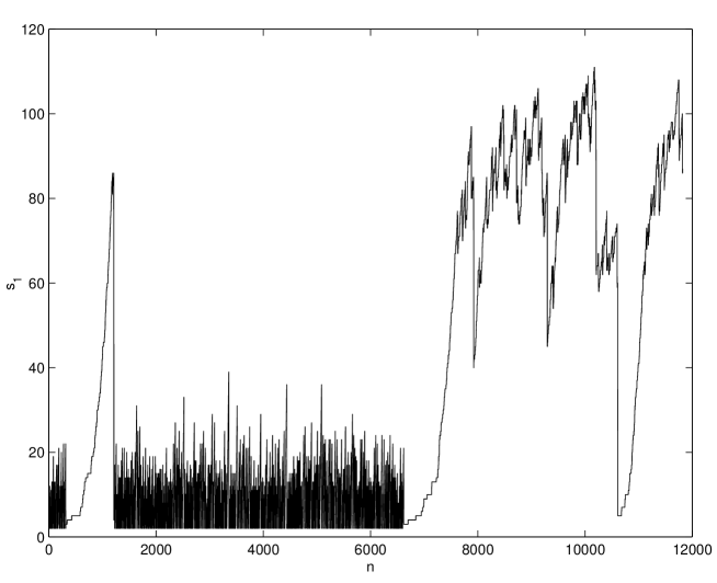
b)
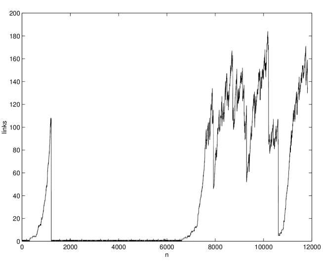
This variant too shows the same qualitative behaviour (see Figure 8.11). When there is no ACS in the graph, none of the nodes remain above the threshold for long. The graph remains small, with few nodes and links. The chance formation of an ACS changes things. Again the number of links and the number of nodes are seen to rise sharply as more and more nodes get attached to the dominant ACS. A third region analogous to the organized phase can also be seen, once the ACS grows large enough for some of its nodes to have values below the threshold, but the transition is not so clear because there is no upper cutoff for the number of nodes in the graph.
Because only positive links are allowed all the analytical results, including theorems 3.1 and 4.1, hold for this variant too. In the initial graph, if there is no ACS, most of the nodes will have . All of these nodes will be removed from the graph leaving a graph with very few nodes and only those links assigned to the new node. Throughout the random phase the graph will consist of only very few nodes. As soon as the first ACS forms the graph will consist only of that ACS and the added node. The ACS grows whenever the new node joins it. Here there is a slight difference from the original model. The rare events where several nodes, including the new node, simultaneously join the dominant ACS are not possible in this variant. It is also not possible for an ACS that went extinct for some reason to be resurrected (as happened in Figures 5.6j,u) – in this variant the extinct nodes would all be removed from the graph immediately.
Despite the absence of an explicit upper cutoff, the number of nodes cannot grow indefinitely. Because always, the number of nodes cannot grow much larger than . In the run shown above the threshold is and the number of nodes remains well below .
8.7 Different population dynamics
Replicator equation.
A variant where the qualitative behaviour does change drastically is one where equation (4.1) is replaced by the replicator equation (Hofbauer and Sigmund, 1988):
| (8.3) |
The name ‘replicator’ comes from the fact that the equation models self-replicating species, for example in model ecosystems (Hofbauer and Sigmund, 1988; Drossel and McKane, 2003). Because is proportional to , the relative population of species can only grow if it is non-zero in the first place; once it will always stay zero, as expected for self-replicators. The replicator equation can have a variety of attractors depending on the coupling constants and the initial conditions – fixed points, limit cycles, heteroclinic cycles and chaotic attractors have been observed (Hofbauer and Sigmund, 1988). The replicator equation has also been used in the hypercycle model of the origin of life (Eigen and Schuster, 1979).
The other rules of the model are unchanged, making it an evolving version of the hypercycle model. Figure 8.12 shows a typical run. When there is no ACS the number of nodes with non-zero fluctuates wildly, even reaching as high as 40 or more for short periods of time. However, no graph structure is stable for very long and the graph remains random. The times when there is an ACS are the periods in Figure 8.12 when remains at some small constant value for a large number of graph updates. Yet, nothing resembling a growth phase is seen and the system eventually relapses into the random phase. What is happening is that small (hyper)cycles do form but quickly get destroyed when a graph update creates a parasite. This observed behaviour is consistent with existing work on well-stirred hypercycles and replicator networks (Niesert et al., 1981; Happel and Stadler, 1998; Tokita and Yasutomi, 2003).

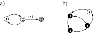
Niesert et al. (1981) have identified three instabilities to which hypercycles are susceptible. Two are of relevance here: Figure 8.13a illustrates the parasite instability mentioned above. For the graph shown here, if , the attractor of equation (8.3) is for generic initial conditions. Thus, the nodes of the core cycle have the least . Figure 8.13b illustrates the short-circuit instability. For generic initial conditions the system always reaches an attractor where node 4, part of the longer cycle, is zero – in general, when long hypercycles are short-circuited by a new link, only the smaller hypercycle survives. These two instabilities are responsible for preventing a large, structured network from forming when the replicator equation (8.3) is used in place of equation (4.1) for the population dynamics.
A generalization of the replicator equation.
The replicator equation is a special case of a more general equation in which the first term is quadratic in the relative population variables:
| (8.4) |
This equation preserves the normalization of because . The equation models a chemistry where two catalysts are (simultaneously) required for the production of each molecular species. It reduces to equation (8.3) in the special case where one of the catalysts is the product itself: , where if and zero if .
In this case, the simplest ACS would consist of three species: species 1 and 2 catalyze species 3, species 2 and 3 catalyze species 1, and species 3 and 1 catalyze species 2 . Consider the case where one periphery node is added to this ACS – let species 1 and 2 also catalyze the production of species 4, and let species 4 not be a catalyst for any of the other species. Numerical simulations show that, unlike the replicator case, here both the core and the periphery nodes have non-zero relative populations in the attractor for generic initial conditions. The ratio of the relative populations of the periphery to the core nodes depends on the link strengths but the core nodes 1, 2 and 3 remain with non-zero relative populations even if the link to the periphery node is stronger than the links between core nodes. Therefore, unlike the special case of the replicator equation, when equation (8.4) is used for the population dynamics it is possible for small ACSs to grow by adding periphery nodes.
Chapter 9 Concluding Remarks
In this thesis I have studied a model of an evolving catalytic network. I have discussed some of the issues and questions of interest related to the evolution of networks in section 1.6. Here, I summarize the interesting phenomena observed in the model, their implications for some of those questions, as well as the limitations and possible extensions of the model.
9.1 Interesting features of the model
-
1.
Rich dynamical behaviour: three phases and multiple timescales. For small the system always appears to be moving from one unstable, or quasi-stable, state to another. It never appears to reach a stable state. Three ‘phases’ of behaviour are observed (see section 5.4). A ‘random phase’ in which the graph remains sparse and consists only of trees, chains and isolated nodes. The ‘growth phase’ is triggered by the chance formation of a small ACS which then grows by accreting nodes to itself. Finally, the ‘organized phase’ begins when the ACS spans the entire graph. There are transitions from each phase to other phases (except that there is never a transition from the growth phase to the random phase). The appearance of different structures dynamically generates multiple timescales: in the random phase, in the growth phase and in the organized phase (see sections 6.2 and 7.5).
-
2.
Growth of structure, interdependence and cooperation. Starting from an initial random graph, the system spontaneously self-organizes into a highly structured graph. This process is triggered by the chance, but inevitable, formation of an ACS, which then grows by accreting other nodes to it, until eventually the entire graph becomes an ACS (section 6.2). The resultant fully autocatalytic graph is highly non-random, occupying an exponentially small (as a function of ) volume of graph space (section 6.3.1). Nevertheless starting from a sparse graph the dynamics inevitably leads the system into this exponentially small volume in a time that grows only as . The growth of exponentially unlikely chemical organizations on the prebiotic Earth in a short time is a puzzle that has been discussed in section 1.9. The growth of autocatalytic sets in this model might shed some light on this puzzle – the implications for the origin of life are discussed further in section 9.2. Along with the growth of non-random structure, the interdependence of the species also grows with the ACS. The fully autocatalytic sets that form have an interdependency almost two orders of magnitude larger than that of random phase graphs (sections 5.4 and 6.3.3). A variant of the model, where negative links are also allowed, exhibits the emergence of cooperation. The formation and growth of ACSs in this variant is accompanied by an increase in the number of cooperative, positive links between species and a decrease in the number of destructive, negative links. The ratio of cooperative to destructive links rises from unity, in the random phase, to an order of magnitude larger in the organized phase (section 8.3). The formation and growth of ACS might be one of the mechanisms responsible for the spontaneous emergence of cooperation in a variety of contexts.
-
3.
Structure of fully autocatalytic graphs. The graphs produced at the end of the growth phase have several interesting structural features. Firstly, they are fully autocatalytic. However, they are not random fully autocatalytic graphs, as evidenced by their broad, though not scale-free, out-degree distribution which is displayed in Figures 6.6 and 6.7 (however, whether runs from other parameter ranges produce scale-free graphs or not remains an open question). An interesting feature is that the in-degree distribution spans a much smaller range than the out-degree distribution. While the fully autocatalytic graphs have a small clustering coefficient (section 6.3.2), they do consist of an irreducible core that is more clustered, from which grow the chains and trees that form the periphery. These observations suggest that, in addition to the commonly studied properties of small-worldness and scale-freeness, it might be interesting to examine real networks for properties such as autocatalysis, a core-and-periphery structure, a difference between the in- and out-degree distributions, etc.
-
4.
Large extinctions: destruction of ACSs. ACSs not only form and grow, but over long times also get destroyed. The destruction of an ACS is usually sudden and accompanied by the extinction of a large number of species, a ‘crash’. The asymmetry between rises and drops of as well as fat tails in the distribution of crash sizes (Figure 7.1) are seen in the fossil record (Newman and Palmer, 1999) and in financial markets (Bouchaud, 2001; Johansen and Sornette, 2001). An interesting feature of the distribution of drops in is it’s bimodal structure for low – the probability of large drops in is an order of magnitude greater than intermediate size drops. A similar bimodality is observed in distribution of earthquake sizes in an earthquake model described by Carlson and Langer (1989), but the mechanism causing it is different.
-
5.
Causes of large extinctions: core-shifts, innovations and keystone species. A variety of mechanisms have been suggested as causes of large extinction events in macroevolution (Maynard-Smith, 1989; Glen, 1994) and finance (Bouchaud, 2001; Johansen and Sornette, 2001). The largest of the extinction events in this model are usually core-shifts – a discontinuous change of the core of the dominant ACS in a single graph update. It is interesting that such core-shifts can be caused both by the removal of an important ‘keystone’ species as well as by graph structures created by the new species, ‘innovations’ (section 7.4). One can distinguish two processes involving innovations, both having analogues in the real world. One is exemplified by the appearance of the automobile that made the horse drawn carriage and its ancillary industries obsolete. This is like the example of the core-transforming innovation shown in Figure 7.7 where the graph update produced an irreducible structure that was ‘stronger’ than the existing core. This structure became the new core, driving the old core and nodes dependent on it to extinction. The subsequent development of other industries dependent on the automobile mirrors the growth of the ACS around the new core. The second process is exemplified by the emergence of the body plans of several phyla that are dominant today. It is believed that while these body plans originated in the Cambrian era more than 520 million years ago (Valentine et al., 1999), the organisms with these body plans played no major role till about 250 million years ago. They started flourishing only when the Permian extinction depleted the other species that were dominant till that time (Erwin, 1996). This is similar to the events shown in Figure 7.8 where an earlier innovation had lain dormant for a while without disturbing the existing core, but when the latter became sufficiently weak, took over as the new core.
-
6.
Predicting crashes. Certain graph theoretic markers could possibly be used to predict whether a crash is imminent (section 7.7). The Perron-Frobenius eigenvalue, , is one such marker. Most of the large extinctions are core-shifts, caused by the removal of keystone species, takeover by core-transforming innovations, or takeover by dormant innovations. The graph is most susceptible to these core-shifts when its or close to it. The dependency distribution is another marker: it is bimodal for graphs preceding a crash. The in and out-degree distributions also appear to fall off faster, as a function of degree, for graphs just before a crash, than for the fully autocatalytic graphs produced in the same runs. In combination, these different markers might indicate whether a given graph has an enhanced probability of suffering a crash.
-
7.
Analytical tractability of the model. The analytical tractability of the model is a result of the linearity of the dynamics. Equation (4.1) is nonlinear but, as it originates via a nonlinear change of variables from a linear equation, equation (4.2), its attractors can be easily analyzed in terms of the underlying linear system. The attractors are always fixed points and are just the Perron-Frobenius eigenvectors of the adjacency matrix of the graph. Theorems 3.1 (the eigenvector profile theorem) and 4.1 (the attractor profile theorem) form the backbone of the analytic results about the population dynamics. Note that while the dynamics in the present model is essentially linear as long as the graph is fixed, it is highly nonlinear over long timescales. Because of the coupling of the population and graph dynamics, over long timescales the ‘coupling constants’ in equation (4.2) are not constant but implicitly depend upon the , thus making the evolution highly nonlinear. The simplifying device of widely separated timescales for the graph dynamics and the population dynamics (the population variables reach their attractor before the graph is modified) results in a piecewise linear dynamics that is easier to analyze. The analytic results about the population dynamics have been used in the analysis of the graph dynamics: results such as proposition 6.1, as well as average timescales of appearance and growth of an ACS use insight about the attractors of the population dynamics to predict aspects of the graph dynamics.
-
8.
Predictability and historicity in the network evolution. There is an interesting mixture of predictability and historicity in the model dynamics. The detailed structure of the dominant ACS is dependent on the chance events that happen throughout the run. Many complicated processes are possible, such as formation of new disconnected ACSs or the reinforcement of an old overshadowed ACS before it was completely broken up (Figures 5.6j,u). Thus, the actual growth of the ACS is usually very complicated with the dominant ACS often undergoing drastic changes in structure caused purely by chance events. However, despite the historical particularities of a given run several aspects are predictable. The non-decreasing nature of in the growth phase is a rule that holds for every run with any values of the parameters and (see proposition 6.1, section 6.2). Other results, such as the timescales of appearance and growth of the ACS, are predictable for ensembles of runs with the same value of and (section 6.2). Also, as discussed above, the transitions from the organized to the growth or random phases that involve the sudden extinction of a large number of species, might be predictable.
-
9.
Correlation between graph structure of perturbations and their impact on the evolution of the network. The network evolves by periodic perturbations, that involve the removal and addition of nodes, and there is a correlation between the graph theoretic nature of the perturbation and its short and long term impact. The perturbations can be broadly placed in two classes based on their effect on :
(i) ‘Constructive perturbations’: these include the birth of a new organization (an innovation of type 6), the attachment of a new node to the core (an innovation of type 4) and an attachment of a new node to the periphery of the dominant ACS (an innovation of type 2).
(ii) ‘Destructive perturbations’: these include complete crashes and takeovers by dormant innovations (both caused by the loss of a keystone node), and takeovers by core-transforming innovations (innovations of type 5). The word ‘destructive’ is used only in the sense that several species become extinct on a short timescale (a single graph update) after such a perturbation. In fact, over a longer timescale (ranging from a few to several hundred graph updates), the ‘destructive’ takeovers by innovations usually trigger a new round of ‘constructive’ events like incremental innovations (type 2) and core enhancing innovations (type 4).
The maximum upheaval is caused by those perturbations that introduce new irreducible structures in the graph (innovations of type 4, 5 and 6) or those that destroy the existing irreducible structure. For example, the creation of the first ACS at triggered the growth phase in the run of Figure 5.3b. Other examples of large upheavals are core-shifts due to takeover by a core-transforming innovation at , takeover by a dormant innovation at , and a complete crash at . -
10.
Context dependence of the effective dynamics of the network evolution. It is characteristic of evolutionary systems, such as this model, that as different (graph) structures spontaneously appear, the nature of selective pressure on existing structures and hence the effective dynamics changes. In the present model the effective dynamics appears to be different in each of the phases even though the microscopic rules remain the same. Thus, in the random phase, because there is no ACS, the graph updates are almost random. In the growth phase there is competition between ACS and non-ACS structures. The dynamics essentially involves the growth of the dominant ACS by the accretion of nodes outside it. Once the entire graph becomes an ACS and the organized phase begins, the effective dynamics once again changes. Now there are no nodes outside the dominant ACS, yet some node has to be removed at each graph update. The competition now shifts to within the ACS – between core and periphery nodes. Typically the core nodes are protected by a higher relative population, therefore most of the graph updates involve periphery nodes. As the periphery realigns itself around stronger core nodes it can happen that a weak core node may be removed at some graph update. Over a long period of time such events may cause the core to become fragile and susceptible to core-shifts. Thus ACSs, which were robust in one phase, become fragile in another. Robust and fragile structures are also found in highly designed systems (Carlson and Doyle, 1999). A different system, in which the selective pressures and effective dynamics change as different structures arise, is discussed by Cohen, M., et al. (2001).
-
11.
Robustness of the ACS growth mechanism to changes in model rules. The basic model has a number of simplifying features that depart from realism but enhance analytical tractability. These are listed in chapter 8 along with variants of the model that relax those simplifications. As shown in that chapter, in most cases relaxing the various idealizations does not change the qualitative behaviour. A variant where the qualitative behaviour does change drastically is one where equation (4.1) is replaced by the replicator equation, making it an evolving version of the hypercycle model (Eigen and Schuster, 1979). In this case small (hyper)cycles do form but quickly get destroyed when a graph update creates a parasite. Consequently, large complex networks cannot form. However, the replicator equation is a special case of a more general equation. In the more general case, unlike the hypercycle model, the ACSs that arise do not get destroyed by parasites (nodes belonging to the periphery). This robustness, one expects, would allow them to evolve into complex networks, as in the original model.
9.2 Implications for the origin of life
As discussed in chapter 1, one of the possible scenarios for which the model might be relevant is for the evolution of a chemical network in a pool on the prebiotic Earth. From the point of view of the origin of life problem the main conclusions are:
-
1.
The model shows the emergence of a chemical organization where none exists. A small ACS emerges spontaneously by random processes and then grows until the entire system is autocatalytic.
-
2.
The graph structures that emerge (ACSs) are collective self-replicators even though none of their components (individual nodes) are self-replicators.
As mentioned in section 1.9, one of the puzzles of the origin of life is the emergence of structured non-random chemical organizations in a relatively short time. A highly structured organization, whose timescale of forming by pure chance is exponentially large (as a function of the size of the system), forms in this model on a very short timescale that grows only logarithmically with the size of the system. Under the assumption that the present model captures what happens in a prebiotic pool, the timescale for a fully autocatalytic chemical organization to grow in the pool is , in units of the graph update time step. This time unit corresponds to the periodicity of the influx of new molecular species, hence it ranges from a day (for tides) to a year (for floods). Further, in the present model the ‘catalytic probability’ is the probability that a random small peptide or RNA molecule will catalyze the production of another, and this has been estimated by Kauffman (1993) as being in the range to . With this range of values for , the timescale, , for a fully autocatalytic chemical organization to grow in the pool lies in the range to years. The time taken for the first cells to arise on Earth, a few hundred million years after the oceans condensed (Joyce, 1989; Schopf, 1993), lies within this range. However, to years is a very wide interval. A tighter prediction, and therefore a better test of the model, would require a more accurate value for the catalytic probability for peptides and catalytic RNA, and a chemically more realistic model.
These speculations might be complementary to some other approaches to the origin of life. Autocatalytic organizations of polypeptides could enter into symbiosis with the autocatalytic citric acid cycle proposed by Wächterhäuser (1990) and Morowitz et al. (2000). The latter would help produce, among other things, amino acid monomers needed by the former; the former would provide catalysts for the latter. It is conceivable that lipid membranes (that have been argued by Segré et al., 2000, 2001, to have their own catalytic dynamics) could form and surround autocatalytic sets, of the kind discussed here, in an enclosure. These ‘cells’ may contain different ACSs, or different parts of the same ACS, thereby endowing them with different fitness levels; such a population could evolve by natural selection. It is also conceivable that such autocatalytic sets of polypeptides formed an enabling environment for the formation and maintenance of self-replicating molecules such as those needed for an RNA world.
9.3 Limitations of the model as a description of a chemical network
I have interpreted the model as a chemical system, with nodes representing molecular species and the links representing catalytic interactions. This interpretation raises some questions. For example, what does it mean to remove a node from the graph? This effectively means that that molecular species cannot be produced again for a finite time until, at some later graph update, a new node comes in with exactly the same links as the one removed. If the species to be removed has a catalyst, then this is inconsistent with the assumption that there is a constant supply of all required reactants. In the random and growth phases this does not happen – in all cases the removed node either has no incoming links, or the values of all its catalysts are zero. In the organized phase too, for runs with small (), a large fraction of graphs have in which case the node that is removed (one of the nodes outside the dominant ACS) either has no incoming links or, if it does, all its catalysts have (otherwise the node would be part of the dominant ACS). However, when , i.e., all nodes have non-zero values, then the removed node always has a catalyst with a non-zero value. Most of the time such removals do not significantly disturb the graph structure. However, in some cases they have drastic effects – for instance, complete crashes (section 7.4.1).
Another question concerns the structure of the molecules in the system. In this model, the identity of the molecular species is defined solely by their interactions and their structure is not specified at all. In reality, it is the structure of molecules that determines their chemical properties. The absence of structure in the model precludes its use in addressing a different problem of the origin of life: How did long proteins with strong and highly specific catalytic properties form from the short, weakly catalytic polypeptides existing initially?
Other weaknesses of the interpretation of the model as a chemical system lie in the assumptions behind the functional form of , in particular, the dependence of only on the relative populations of catalysts of and not on the reactants. Such an assumption implies that the reactants are all present and have unchanging concentrations, i.e., they are buffered and there is effectively a constant supply of reactants. This can lead to the uncontrolled growth in the population of some, or all, molecular species. In reality, the reactants will eventually get consumed thereby truncating the growth of population. Further, the dependence of the growth rate on reactants would make the dynamics nonlinear and hence oscillations and chaotic dynamics might occur. The form of precludes the possibility of this kind of dynamics. The choice of also does not allow for the possibility of other types of chemical reactions, such as conversion of one substrate to another, or cleavage and ligation of molecules, which might be important for the prebiotic pool scenario.
Another limitation is the absence of spatial degrees of freedom. Thus, the model applies only to a well-stirred chemical reactor and cannot address the emergence of spatial structure and its effect on the dynamics of the system. As prebiotic pools need not be well-stirred it would be more appropriate to use reaction-diffusion equations to model the dynamics (Bhalla, 2003).
These are the most serious limitations. Apart from them, the model has several simplifications that aid in the analysis of its dynamical behaviour. These are listed below:
-
1.
All catalysts have the same catalytic efficiency.
-
2.
Inhibitors – negative links – are not present in the model.
-
3.
Self-replicators are not allowed.
-
4.
The selection is extremal; the node with the least is removed at each graph update.
-
5.
The total number of nodes is fixed; the rate of node removals and node additions is exactly the same.
Variants of the model, in which the rules are modified to relax these simplifications, were described in chapter 8 and show the same qualitative behaviour as the original model. Therefore, these are not serious limitations.
9.4 Possible extensions of the model
The above limitations of the model suggest possible directions in which it would be worthwhile to extend the model. Firstly, the structure of the molecular species could be explicitly introduced into the model. This would require specifying some rules to determine the catalytic properties of a molecule from its structure. The structure of the molecular species should determine the reactions in which the molecule will participate. Then there would be no need to remove a node from the graph. In such a model one could explicitly study the evolution of certain structural features of molecules in the system – for instance their length.
Another direction in which to extend the model as a description of a chemical system would be to introduce the reactants explicitly, and also include other kinds of reactions, e.g., reactions in which one molecular species is converted to another type of molecular species. In the reductive citric acid cycle discussed above, a crucial reaction involves the splitting of citrate into two smaller molecules, which then undergo various reactions until each is re-converted into citrate. Therefore, including these kind of reactions is necessary to study the emergence of this kind of autocatalytic set in a chemical network. These changes fit within the general framework described in section 1.7.
Going beyond that framework, spatial degrees of freedom could be added to the model by using reaction-diffusion equations for the dynamics. However, it is computationally difficult to solve such equations for complicated geometries (Press et al., 1992). A compromise might be achieved by simulating a finite number of compartments, within each of which the system is well mixed, and allowing some exchange or diffusion across compartment boundaries (Bhalla, 2003). Then different ACSs could exist in different compartments and interact with each other. This is likely to be computationally easier to simulate and at the same time allows some spatial differentiation.
9.5 Modeling other systems within the same framework
The general framework described in section 1.7 can be used to model systems other than chemical networks. For example, an ecosystem could be modeled. In that case the nodes would represent biological species while the links would represent interactions such as prey-predator, competitive or symbiotic interactions between species. Here removing a node that has become extinct is not a problem because the species are self-replicators (once a species becomes extinct its chance of being recreated can be neglected). However, the self-replicating character of the species in this interpretation must also be reflected in the population dynamics. The Lotka-Volterra equation, replicator equation or other more complicated dynamical equations may be tried (Drossel and McKane, 2003). In modeling an ecosystem one might also wish to modify the way the new node is assigned links. While a random assignment might be interpreted as the invasion of the ecosystem by an entirely alien species, one might also want to include the possibility of an existing species mutating.
Another system that might be modeled in this manner is a genetic regulatory network. The nodes would represent the genes. The would represent the level of expression of a gene, and the links would represent regulatory interactions between the protein product of one gene and another gene. Here again one might wish to allow a new node (a new gene) to be a mutated copy of an existing gene. One might also wish to include other processes that change the graph such as gene duplications.
A third way to modify the graph dynamics would be to allow the rewiring of existing links. This might be most relevant when using the model to describe an economic system, with the nodes representing economic ‘agents’ such as buyers and sellers, or companies, or nations.
Appendix A Proofs of Propositions
- Proposition 2.1:
-
If a graph, ,
(i) has no closed walk then ,
(ii) has a closed walk then .
(i) If a graph has no closed walk then all walks are of finite length.
Let the length of the longest walk of the graph be denoted . If
is the adjacency matrix of a graph then equals
the number of distinct walks of length from node to node
. Clearly for . Therefore all eigenvalues of
are zero. If are the eigenvalues of
then are the eigenvalues of . Hence, all
eigenvalues of are zero, which implies . This
proof was supplied by V. S. Borkar.
(ii) If a graph has a closed walk then there is some node that
has at least one closed walk to itself, i.e. ,
for infinitely many values of . Because the trace of a matrix
equals the sum of the eigenvalues of the matrix, ,
where are the eigenvalues of . Thus, ,
for infinitely many values of . This is only possible if one of
the eigenvalues has a modulus . By the Perron-Frobenius
theorem, is the eigenvalue with the largest modulus,
hence . This proof was supplied by R. Hariharan.
- Proposition 2.2:
-
If all the basic subgraphs of a graph are cycles then , and vice versa.
For any cycle of nodes whose adjacency matrix is , it follows that is the identity matrix (for each there is a closed walk of length from node to itself, and there are no other walks of length ). Therefore, each eigenvalue, , of satisfies , i.e., . The Perron-Frobenius eigenvalue of must be real, therefore, . Thus, if all basic subgraphs of a graph are cycles then .
If then the basic subgraphs must be irreducible,
they cannot be single nodes. Assume that one of the basic subgraphs
is not a cycle. Let its adjacency matrix be . Because is
irreducible, every row has at least one non-zero entry. Construct
by removing, from each row of , all non-zero entries except
one that can be chosen arbitrarily. Thus has exactly one non-zero
entry in each row. Clearly the column vector
is a right eigenvector of with eigenvalue 1 and hence .
Also , therefore, by the Perron-Frobenius theorem for irreducible
matrices, .
But this contradicts the earlier assumption that .
Hence, if , all the basic subgraphs must be cycles.
- Proposition 3.1:
-
(i) All cycles are irreducible graphs and all irreducible graphs are ACSs.
(ii) Not all ACSs are irreducible graphs and not all irreducible graphs are cycles.
(i) Clearly in a cycle, there is a path from every node to any
other node hence all cycles are irreducible. In every irreducible
graph each node must have an incoming link from one of the other nodes.
Hence all irreducible graphs are ACSs.
(ii) This is proved by providing two counterexamples. Figure A.1a
shows an ACS that is not an irreducible graph, and Figure A.1b
shows an irreducible graph that is not a cycle.
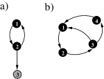
- Proposition 3.2:
-
(i) An ACS must contain a closed walk. Consequently,
(ii) If a graph has no ACS then .
(iii) If a graph has an ACS then .
(i) Let be the adjacency matrix of a graph that is an ACS. Then by definition, every row of has at least one non-zero entry. Construct by removing, from each row of , all non-zero entries except one that can be chosen arbitrarily. Thus has exactly one non-zero entry in each row. Clearly the column vector is an eigenvector of with eigenvalue 1 and hence . Proposition 2.1 therefore implies that contains a closed walk. Because the construction of from involved only removal of some links, it follows that must also contain a closed walk. (ii) and (iii) follow from part (i) and propositions 2.1(i) and (ii), respectively.
- Proposition 3.3:
-
If , then the subgraph of any PFE of is an ACS.
Let x be a PFE of a graph. Renumber the nodes of the graph so that only for . Let be the adjacency matrix of this graph. As x is an eigenvector of the matrix
Because for and ,
it follows that for each .
Therefore, for each there exists a such
that . Hence the submatrix ,
, has at least one non-zero entry in each row. Thus
each node of the subgraph corresponding to this submatrix has an incoming
link from one of the other nodes in the subgraph. Hence the subgraph
is an ACS.
- Lemma A:
-
Let be a submatrix of a non-negative matrix . Denote the Perron-Frobenius eigenvalue of by and that of by . Then .
Renumber the nodes so that can be written as:
Consider the matrix
and denote its Perron-Frobenius eigenvalue by .
Because we have
from the Perron-Frobenius theorem.
Also .
Hence, .
Therefore .
- Proposition 3.4:
-
Let x be a PFE of a graph , and let denote the adjacency matrix of the subgraph of x. Let denote the Perron-Frobenius eigenvalue of . Then and must contain at least one of the basic subgraphs of .
Let the nodes be numbered such that only for .
Because x is an eigenvector of the matrix we have
(
has been abbreviated to ).
.
Therefore is an eigenvector of
the submatrix , with eigenvalue .
Also by lemma A, . Therefore .
It follows that the subgraph must contain a strong component
with Perron-Frobenius eigenvalue . That strong component
would be present in also and would be one of it’s basic subgraphs.
Hence there exists at least one basic subgraph of that is non-zero
in any PFE of .
- Lemma B:
-
Let be an non-negative irreducible matrix with Perron-Frobenius eigenvalue and let . Then either or .
As is the adjoint of and , it follows that and . Hence any column of is either a PFE of or is a column of zeroes. If it is a PFE then by the Perron-Frobenius theorem it is either strictly positive or strictly negative. A similar result holds for the rows of . Hence either or has all elements non-zero. If has all elements non-zero then it follows that either or .
I now show that one element of is non-zero. The element of is where is the matrix with the last row and column deleted. Consider the matrix
Clearly . Because is irreducible it cannot have a zero column or row; if it did there would be no path to or from that node to other nodes. Hence , which implies, as a consequence of the Perron-Frobenius theorem for irreducible matrices, that is not an eigenvalue of and, therefore, is not an eigenvalue of either. Hence .
Therefore, either or .
- Proposition 3.5:
-
If a node is non-zero in a PFE then all nodes it has access to are non-zero in that PFE.
Let be a node that is non-zero in the PFE . Let
be any node downstream from it. Therefore there exists a positive
integer such that .
Assume that . As ,
,
, for each . This
is a contradiction because and . Hence
.
- Proposition 3.6:
-
If a node is upstream from a basic subgraph then that node is zero in any PFE.
Let the nodes be renumbered so that the last few – nodes – form a basic subgraph of the graph . Let node be some other node that is upstream from this basic subgraph, i.e., there exists a positive integer such that . Let be a PFE of . Then:
The equations for can be written in matrix form as follows:
where ,
and is the adjacency
matrix of the basic subgraph.
| (A.1) |
with .
Let us assume that node is non-zero in the PFE, i.e. . Also , therefore .
Let denote the row of .
Because ,
| (A.2) |
with at least one being non-zero.
(A.1) gives
Multiply the above equation by and sum from to .
| (A.3) |
Let . By definition
Comparing with (A.4) we have
because from lemma B either or (as is irreducible it follows that is irreducible hence lemma B is applicable).
Therefore from (A.3)
However, we are given that . Hence the assumption that has led to a contradiction. The only other possibility is that in the PFE.
- Proposition 3.7:
-
If a node does not have access from a basic subgraph then it is zero in any PFE.
Let the submatrix consist of all the strong components that do not have access from any basic subgraph of . The matrix can be written as:
where consists of all the basic subgraphs of and all the nodes having access from them. Let be a PFE of . The eigenvector equations give:
| (A.5) |
has no basic subgraphs of , hence is not
an eigenvalue of . Therefore (A.5) has only the trivial solution
.
- Theorem 3.1:
-
Eigenvector profile theorem
For any graph , determine all the basic subgraphs of . Denote them by . Determine which of these does not have any other downstream from it. Denote these by . Then:
(i) For each there exists a unique (upto constant multiples) PFE in which the nodes of and all nodes having access from them are non-zero and all other nodes are zero. It is evident that these PFEs are simple. Moreover these are the only simple PFEs of the graph .
(ii) Any PFE is a linear combination of these simple PFEs.
The first statement follows from propositions 3.4–3.7. To prove the second statement, I first write the matrix as follows:
contains all the nodes that don’t have access from any . Thus all nodes in will be zero in any PFE . contains all nodes having access from some , i.e. . As the eigenvector equations for each are:
Because each is irreducible the above equations have solutions that are unique upto constant multiples. Denote these solutions by . The equations for are:
where .
Consider the case where only one of the is non-zero. Denote the b for that case by and the corresponding (unique) solution of the above equations by . For the general case where more than one is non-zero, b will be a linear combination of the because , for each node in each , is unique upto constant multiples. Hence the general solution for will also be a linear combination of . Rothblum (1975) provides a different proof that uses the principle of mathematical induction.
- Proposition 3.8:
-
Every node in the core of a simple PFE has access to every other node of the PFE subgraph. No periphery node has access to any core node.
From theorem 3.1 it follows that the subgraph of any simple PFE is the subgraph induced by the nodes of one of the basic subgraphs (defined in the statement of theorem 3.1) and all nodes having access from . The core nodes are the nodes of Because is irreducible, it is evident that every core node has access to every other core node. Further, every periphery node has access from some, and therefore all, nodes of . Thus, each core node has access to every other node of the PFE subgraph.
Now assume there is some periphery node that has access to some
core node . Also has access to , therefore is strongly
connected to . In that case would also be part of the basic
subgraph , i.e., would be a core node, not a periphery
node. Thus, no periphery node can have access to any core node.
- Proposition 4.1:
-
For any graph ,
(i) Every eigenvector of that belongs to the simplex is a fixed point of equation (4.1), and vice versa.
(ii) Starting from any initial condition in the simplex , the trajectory converges to some fixed point (generically denoted X) in .
(iii) For generic initial conditions in , X is a Perron-Frobenius eigenvector (PFE) of .
(iv) If has a unique (upto constant multiples) PFE, it is the unique stable attractor of equation (4.1).
(v) If has more than one linearly independent PFE, then X can depend upon the initial conditions. The set of allowed X is a linear combination of a subset of the PFEs. The interior of this set in may then be said to be the ‘attractor’ of (4.1), in the sense that for generic initial conditions all trajectories converge to a point in this set.
The proof uses the Jordan canonical form of the matrix (Horn and Johnson, 1985):
with .
Each is called a Jordan block and is an matrix of the form:
The are the eigenvalues of . The need not be distinct; there may be more than one Jordan block with the same diagonal. It is known that any complex matrix can be put in the above form by a similarity transformation, i.e. there exists a non-singular matrix such that , and moreover, the form of is unique barring rearrangements of the Jordan blocks (Horn and Johnson, 1985). The columns of form ‘Jordan chains’ that satisfy the following equations:
Thus are eigenvectors of with eigenvalues respectively. It can be shown that there is one and only one linearly independent eigenvector of associated with each Jordan block and vice versa (Horn and Johnson, 1985). The other columns of are called ‘generalized eigenvectors’ of .
Now consider the underlying dynamics (4.2) from which (4.1) is derived: Because (4.1) is independent of , we can set in (4.2) without any loss of generality. With the general solution of (4.2), which is a linear system, can be schematically written as:
where and are column vectors.
Using the Jordan canonical form of in the general solution of (4.2) we find:
Now
where
Let
Then the attractor of (4.1) will be and only the fastest growing components in will contribute to . Therefore, in calculating , I will keep only the fastest growing terms and set all others to zero for convenience.
First consider the case where is unrestricted – any initial condition is allowed. Then some components of could be zero. If all the components corresponding to a particular Jordan block are zero in then that Jordan block will not contribute to . Further, among the Jordan blocks that do have some non-zero components in , only the ones with the largest will survive in the limit because of the term. Let the Jordan blocks that survive be the first ones (the nodes can always be renumbered to achieve this). From the structure of it then follows that the only non-zero components of will be the components . Therefore , with being summed over the set . are constants and is the th column of . Then, the attractor is , where is a constant chosen to make , and . Notice that are all eigenvectors of with eigenvalue Therefore is a fixed point, and is an eigenvector of . This proves (i) and (ii).
Now consider the case of generic initial conditions. In this case . The only terms to survive will be in the Jordan blocks corresponding to the Perron-Frobenius eigenvalue, , of . Moreover, of these blocks only the largest sized blocks will survive. Suppose the largest Jordan blocks corresponding to eigenvalue have size . Let the Jordan blocks be arranged such that these blocks are the first few. Then, in the limit , will have the following form:
Thus if there are Jordan blocks of size corresponding to eigenvalue then, for the purpose of calculating , all elements of can be set to zero except the elements which will be equal to . Therefore the only non-zero elements of , in the limit, will have values for , where are real constants that depend on . Thus,
Therefore,
where is a constant chosen to make . Thus is a linear combination of those PFEs of that correspond to the largest Jordan blocks with eigenvalue . This proves (iii) and (iv).
- Theorem 4.1:
-
Attractor profile theorem
1) Determine all the strong components of the given graph . Denote these by .
2) Determine which of these are basic subgraphs. Denote them by .
3) Construct a graph, denoted , with nodes, representing the , and a link from node to node if there is a path from any node of to any node of that does not contain a node of any other basic subgraph.
4) Determine which of the are at the ends of the longest paths in the above graph . Denote these by .
For each there exists a unique (upto constant multiples) PFE that has only nodes of and all nodes having access from them non-zero, and all other nodes zero. The attractor set consists of all linear combinations of these PFEs that lie on the simplex .
It has already been shown (proposition 4.1) that the attractor is a linear combination of those PFEs of that correspond to the largest Jordan blocks with eigenvalue . Therefore to prove this theorem it suffices to show that the PFEs corresponding to the largest Jordan blocks with eigenvalue are precisely those PFEs corresponding to the subgraphs that are at the ends of the longest paths in .
It can be shown that the size of the largest Jordan block with eigenvalue is equal to the length of the longest path in the graph (see Rothblum, 1975, where it is called the index of ). It is also shown by Rothblum that for each basic subgraph there is a sequence of generalized eigenvectors , where is the length of the longest path in starting at , such that , (where ) and if and only if the longest path from a node of to node when projected onto the graph has a length .
Let the length of the longest path in be and consider one such path starting at, say, and ending at some . Then, corresponding to this path, there is a sequence of generalized eigenvectors that includes the PFE in which only and nodes having access from it are non-zero. Thus there is a Jordan block of size corresponding to the PFE in which only and all nodes having access from it are non-zero. This is also the largest Jordan block. Therefore the PFEs corresponding to the largest Jordan blocks with eigenvalue are precisely those PFEs corresponding to the subgraphs that are at the ends of the longest paths in . The attractor set will consist of linear combinations of these PFEs.
- Proposition 4.2:
-
For any graph with , in the attractor only the nodes at the ends of the longest paths are non-zero. All other nodes are zero.
Consider a graph consisting only of a linear chain of nodes,
with links, pointing from node 1 to node 2, node 2 to 3, etc.
The node 1 (to which there is no incoming link) has a constant population
because the r.h.s of (4.2) vanishes for (taking
). For node 2, we get , hence
for large . Similarly, it can be seen that grows as .
In general, it is clear that for a graph with no cycles,
for large (when ), where is the length of the
longest path terminating at node . Thus, nodes with the largest
dominate for sufficiently large . Because the dynamics (4.1)
does not depend upon the choice of , for all
except the nodes at which the longest paths in the graph terminate.
- Proposition 4.3:
-
For any graph ,
(i) For every X belonging to the attractor set, the set of nodes for which is the same and is uniquely determined by . The subgraph formed by this set of nodes will be called the ‘subgraph of the attractor’ of (4.1) for the graph .
(ii) If , the subgraph of the attractor is an ACS.
This is a corollary to theorem 4.1. The set of nodes for which
consists of nodes in all the subgraphs described
in the statement of theorem 4.1, and all nodes having access from
them. This set evidently depends only on . Further
is a PFE of . Therefore, from proposition 3.3 the subgraph of
the attractor is an ACS if .
- Proposition 6.1:
-
is a non-decreasing function of as long as .
Let the adjacency matrix of the graph at time step be denoted and its Perron-Frobenius eigenvalue be denoted . Removing a node with the least from this matrix gives an matrix that I denote .
From lemma B, .
Because the removal of the node with the least
leaves the dominant ACS (denoted ) unaffected, i.e.,
is a subgraph of .
However is an eigenvalue of . Hence,
,
.
Now a new node is added to to get . Because is
a subgraph of , it follows that ,
.
- Proposition 7.1:
-
Let denote the maximal new irreducible subgraph that includes the new node at time step . will become the new core of the graph, replacing the old core , whenever either of the following conditions are true:
(a) or,
(b) and is downstream of .
After a node is removed from the graph , the resultant graph is which has the core . Now a new node is added to this graph to get . This graph contains the irreducible subgraph . Clearly if then is the only basic subgraph of and will therefore be its core. But if then it is only one of the basic subgraphs of . By definition , because it is the core of , contains those basic subgraphs that are at the ends of the longest chains of basic subgraphs in . Therefore, will be a basic subgraph at the end of the longest chain of basic subgraphs in only if it is downstream from some node of . If this is so, then it will be the single basic subgraph at the end of the longest chain, and therefore will be the core of .
Appendix B Programs to simulate the model
This appendix describes two programs, included in the attached CD, that can be used to simulate the model and its variants. The programs differ in the way the attractor is found at each time step. The first program uses theorem 4.1. The second numerically integrates equation (4.1) to find the attractor. These different methods will be described below, in sections B.4 and B.5, but first I will describe what is common to the two programs. Both programs are written in C++, however they can be easily translated to C because I have used only certain small convenient features of C++ and no object oriented code.
B.1 Variables and data types
The two parameters of the model are , the total number of nodes of the graph, which is specified by the variable named n of type int (integer), and , the catalytic probability, which is specified by the variable named lprob of type double (double precision real number).
The dynamical variables are the graph , whose adjacency matrix is stored as a two dimensional array of type double, and the relative populations which are stored as a one dimensional array of type double.
B.2 Creating the initial random graph
The initial random graph is created in the function makec4. For each , I generate a (pseudo)random number of type double uniformly distributed in the interval . If the random number is less than then is assigned unity, otherwise it is assigned zero. For generating (pseudo)random numbers uniformly distributed in the interval I have used the routine ran1 from Numerical Recipes (Press et al., 1992). However, as Press et al. do not allow Numerical Recipes routines to be distributed publicly, I have replaced calls to ran1 in the programs included in the attached CD by calls to the internal random number generator drand48. The function call is drand48() and returns a number of type double uniformly distributed in the interval . The variable idum of type long (long integer) is used to set the initial seed of the random number generator using the function srand48.
B.3 The graph update
Once the attractor is known, the set of nodes with the least has to be determined. Because the are stored as data type double it makes sense to choose a threshold such that two numbers differing by less than the threshold will be considered equal. In the programs, the threshold has been chosen to be . Note that in the case where theorem 4.1 is used to determine the attractor, the set is known exactly in most cases; there are few situations where the threshold is actually required.
After the set is determined, one picks an arbitrary node out of this set for removing from the graph. This node is picked by choosing a random number from the set , where is the size of the set (if is a random number in the interval generated using ran1 or drand48, then int(l*r) is a random integer between 0 and , inclusive).
Once the node to be removed is decided, say node , the graph update is done by the function call update4(k). All the elements of the matrix in that row and column are reassigned to 0 or 1 by the same procedure used to create the initial matrix, i.e., a random number is generated and for each , is assigned unity if the random number is less than , and is assigned zero otherwise, and similarly for . The function update4 also sets to (the variable xin of type double) and rescales all other so that .
B.4 Program that uses the attractor profile theorem
B.4.1 Determining which node to remove
The crucial step involves the determination of the set, , of nodes with the least at each time step. The results from chapter 4, in particular theorem 4.1, are used to do this.
-
1.
Determine all the strong components of the given graph. Denote these by .
-
2.
Determine which of these are basic subgraphs. Denote them by .
-
3.
Construct a graph, , of nodes representing the with a link from node to node if there is a path from any node of to any node of that does not contain a node of any other basic subgraph.
-
4.
Determine which of the are at the ends of the longest paths in the above graph . Denote these by .
-
5.
For each construct a vector with (arbitrary) non-zero values assigned to those components corresponding to nodes in and all nodes having access from them. Set all other components to zero.
-
6.
(a) If there are any nodes that are zero in all these vectors then they form the unique set for generic initial conditions.
(b) If no nodes are zero, then first the PFE corresponding to each is determined using Matlab. This is done by constructing the adjacency matrix of the subgraph induced by all nodes in and all nodes having access from them and using Matlab’s eig function to determine the (unique) PFE of this matrix. Then,
If there is only one , its PFE is used to determine . Because its PFE is unique upto constant multiples, the set is also unique and independent of the (generic) initial conditions.
If there is more than one , then depends on the initial conditions. In this case is taken to be a linear combination of the PFEs corresponding to each , with the coefficients of the linear combination being random numbers generated by ran1 or drand48. The set is then determined from these values of .
This last case only occurs for graphs in which several ACSs coexist and the whole graph is spanned by these ACSs. Such a situation occurs very rarely. Thus when the set is unique and independent of initial conditions. When most of the time there is only one in which case again is unique and independent of initial conditions but has to be determined numerically (using Matlab). Finally, very rarely, when and there is more than one in the graph then the set depends on the initial conditions and an arbitrary linear combination of PFEs is taken as the attractor. The function that implements this algorithm in the program is called thmeig.
Note that the code was written to work with Matlab 5.2 and therefore may require some modifications to work with other versions of Matlab.
B.4.2 Output files
Having specified the values of the variables n (the size of the graph), lprob (the catalytic probability), xin (the relative population assigned to each new node) and idum (the initial random seed), the program produces a run with the specified number of graph updates. Several output files are created, which consist of one or more columns of data. Each row corresponds to an iteration of the graph dynamics and different filenames are used for storing different quantities. The list below shows the naming scheme I have used for the output files:
-
1.
*.l : the total number of links.
-
2.
*.px : column 1 has the number of nodes with , column 2 has the number of nodes with calculated (using theorem 4.1) in thmeig if there is an ACS, or -1 if there is no ACS in the graph.
-
3.
*.lm : the Perron-Frobenius eigenvalue of the graph.
-
4.
*.min : information about each graph update, which node was replaced, which new links were assigned. This can be used to reconstruct all the graphs later using the program mtx.cpp included in the attached CD (see appendix C).
-
5.
*.clno : the number of irreducible subgraphs of the graph.
-
6.
*.clev : the Perron-Frobenius eigenvalue of each irreducible subgraph.
-
7.
*.cn : number of core nodes.
-
8.
*.cs : list of core nodes.
-
9.
*.0num : number of nodes with .
-
10.
*.0nodes : list of nodes with .
Any filename can be substituted for *. I typically use a name that contains information about the values given to n, lprob and idum, thereby allowing me to distinguish one type of run from another.
B.5 Program that finds the attractor numerically
B.5.1 Numerical method for determining the attractor
As an alternative to the above program that uses theorem 4.1, I have included, in the attached CD, a program that numerically integrates equation (4.1) to find its attractor. The program uses a 5th order adaptive Runge-Kutta scheme based on the algorithm given in Numerical Recipes (Press et al., 1992). The function that implements this in the program is called dyneig. A call to dyneig replaces the call to thmeig in the previous program.
I have included this alternate program for two reasons. One, for several variants of the model, such as the variant with negative links (section 8.3), theorems 3.1 and 4.1 do not hold. Then the only option is to use a numerical method to find the attractor – many of the variants discussed in chapter 8 have been simulated using this method.
The second reason is historical. When I initially began working on this model, theorems 3.1 and 4.1 did not exist (in my mind). All the initial runs were done using the numerical method. Some patterns were consistently observed in these runs. For example, whenever there was a 2-cycle downstream from another, and these were the only basic subgraphs, then the upstream 2-cycle was always zero. These observations were the stepping stones that led to the theorems.
B.5.2 Output files
As in the previous program, the following variables must be set before running the program: n (the size of the graph), lprob (the catalytic probability), xin (the relative population assigned to each new node) and idum (the initial random seed). For a given run, the program produces four output files, each of which consist of one or more columns of data, and are named as follows:
-
1.
*.l : the total number of links.
-
2.
*.px : column 1 has the number of nodes with , column 2 has a flag that is 1 if the set of nodes with is an ACS and 0 otherwise.
-
3.
*.S1 : list of nodes having .
-
4.
*.min : information about each graph update, which node was replaced, which new links were assigned. This can be used to reconstruct all the graphs later using the program mtx.cpp included in the attached CD (see appendix C).
Appendix C Contents of the attached CD
The attached CD contains the following files:
-
•
contents: The contents of the CD; this list.
-
•
thesis.pdf: This thesis in PDF format.
-
•
thesis.ps: This thesis in Postscript format.
-
•
Programs/thmruns.cpp: A program to simulate the model, that uses theorem 4.1 (see section B.4).
- •
-
•
Programs/mtx.cpp: A program to extract the adjacency matrix of the graph at any given iteration, from the *.min file produced by thmruns.cpp or rk5runs.cpp. The program requires the seed used to initialize the random number generator for that run.
-
•
Programs/mtx2gw.cpp: A program to convert the adjacency matrix files produced by mtx.cpp to the LEDA format.
-
•
Programs/calcdeg.cpp: A program to calculate the in, out and total degree distributions for some or all graphs of a run from the *.min file produced by thmruns.cpp or rk5runs.cpp. The program requires the seed used to initialize the random number generator for that run.
-
•
Programs/calcdep.cpp: A program to calculate the interdependency and dependency distribution for some or all graphs of a run from the *.min file produced by thmruns.cpp or rk5runs.cpp. The program requires the seed used to initialize the random number generator for that run.
-
•
Programs/rndgraph.cpp: A program to produce a set of graphs drawn from the ensemble , and to calculate the degree and dependency distribution.
- •
- •
-
•
Data/t05s3n100.*: The data files produced by thmruns.cpp for a run with . This is the run displayed in chapter 5 (see Figures 5.2 and 5.3c). Note that these data files, and the ones above, were produced by a version of thmruns.cpp that uses ran1 as the random number generator and, therefore, are likely to differ from runs with the same random seed that are produced by the program provided in the CD, which uses drand48.
-
•
Data/crashes.txt: A list of iterations, for each of the runs t025s*n100.* with , at which the graph update resulted in a crash. The core overlap for each crash is also given.
-
•
Graphs/n*.gw: The graphs of Figure 5.6 in LEDA format.
-
•
Graphs/n*.mtx: The adjacency matrices of the graphs shown in Figure 5.6.
References
- Adamic et al. (2003) Adamic, L. A., Lukose, R. M. and Huberman, B. A. (2003) Local search in unstructured networks, in Handbook of Graphs and Networks, eds. Bornholdt, S. and Schuster, H. G. (Wiley-VCH, Berlin) pp. 295–317.
- Albert and Barabási (2002) Albert, R. and Barabási, A.-L. (2002) Statistical mechanics of complex networks, Rev. Mod. Phys. 74, 47–97.
- Albert et al. (1999) Albert, R., Jeong, H. and Barabási, A.-L. (1999) Diameter of the world wide web, Nature 400, 130–131.
- Albert et al. (2000) Albert, R. Jeong, H. and Barabási, A.-L. (2000) Error and attack tolerance of complex networks, Nature 406, 378–382.
- Amaral et al. (2000) Amaral, L. A. N., Scala, A., Barthélémy, M. and Stanley, H. E. (2000) Classes of small-world networks, Proc. Natl. Acad. Sci. (USA) 97, 11149–11152.
- Arbib (1995) Arbib, M. A., ed. (1995) Handbook of Brain Theory and Neural Networks (MIT Press, Cambridge).
- Bagley and Farmer (1991) Bagley, R. J. and Farmer, J. D. (1991) Spontaneous emergence of a metabolism, in Artificial Life II, eds. Langton, C. G., Taylor, C., Farmer, J. D. and Rasmussen, S. (Addison Wesley, Redwood City) pp. 93–140.
- Bagley et al. (1991) Bagley, R. J., Farmer, J. D. and Fontana, W. (1991) Evolution of a metabolism, in Artificial Life II, eds. Langton, C. G., Taylor, C., Farmer, J. D. and Rasmussen, S. (Addison Wesley, Redwood City) pp. 141–158.
- Bak and Sneppen (1993) Bak, P. and Sneppen, K. (1993) Punctuated equilibrium and criticality in a simple model of evolution, Phys. Rev. Lett. 71, 4083–4086.
- Barabási and Albert (1999) Barabási, A.-L. and Albert, A. (1999) Emergence of scaling in random networks, Science 286, 509–512.
- Bhalla (2002) Bhalla, U. S. (2002) Mechanisms for temporal tuning and filtering by postsynaptic signaling pathways, Biophys. J. 83, 740–752.
- Bhalla (2003) Bhalla, U. S. (2003) Understanding complex signaling networks through models and metaphors, Prog. Biophys. Mol. Biol. 81, 45–65.
- Bhalla and Iyengar (1999) Bhalla, U. S. and Iyengar, R. (1999) Emergent properties of biological signaling pathways, Science 283, 381–387.
- Bhalla et al. (2002) Bhalla, U. S., Ram, P. T. and Iyengar, R. (2002) MAP kinase phosphatase as a locus of flexibility in a mitogen-activated protein kinase signaling network, Science 297, 1018–1023.
- Biswal and Dasgupta (2002a) Biswal, B. and Dasgupta, C. (2002a) Neural network model for apparent deterministic chaos in spontaneously bursting hippocampal slices, Phys. Rev. Lett. 88, 088102/1–4.
- Biswal and Dasgupta (2002b) Biswal, B. and Dasgupta, C. (2002b) Stochastic neural network model for spontaneous bursting in hippocampal slices, Phys. Rev. E 66, 051908/1–18.
- Bollobás (1998) Bollobás, B. (1998) Modern Graph Theory (Springer, New York).
- Bollobás (2001) Bollobás, B. (2001) Random Graphs, Second Edition (Cambridge Univ. Press, Cambridge).
- Bollobás and Riordan (2003) Bollobás, B. and Riordan, O. M. (2003) Mathematical results on scale-free random graphs, in Handbook of Graphs and Networks, eds. Bornholdt, S. and Schuster, H. G. (Wiley-VCH, Berlin) pp. 1–34.
- Bornholdt and Schuster (2003) Bornholdt, S. and Schuster, H. G. (2003) Handbook of Graphs and Networks (Wiley-VCH, Berlin).
- Bose (2002) Bose, I. (2002) Biological networks, Preprint: http://www.arxiv.org/abs/cond-mat/0202192.
- Bouchaud (2001) Bouchaud, J.-P. (2001) Power laws in economics and finance: Some ideas from physics, Quant. Finance 1, 105–112.
- Broder et al. (2000) Broder, A., Kumar, R., Maghoul, F., Raghavan, P., Rajagopalan, S., Stata, R., Tomkins, A. and Wiener, J. (2000) Graph structure in the web, Comput. Netw. 33, 309–320.
- Callaway et al. (2000) Callaway, D. S., Newman, M. E. J., Strogatz, S. H. and Watts, D. J. (2000) Network robustness and fragility: Percolation on random graphs, Phys. Rev. Lett. 85, 5468–5471.
- Camacho et al. (2002) Camacho, J., Guimerà, R. and Amaral, L. A. N. (2002) Robust patterns in food web structure, Phys. Rev. Lett. 88, 228102/1–4.
- i Cancho and Solé (2001) i Cancho, R. F. and Solé, R. V. (2001) The small-world of human language, Proc. R. Soc. London B 268, 2261–2265.
- Carlson and Doyle (1999) Carlson, J. M. and Doyle, J. (1999) Highly optimized tolerance: A mechanism for power laws in designed systems, Phys. Rev. E 60, 1412–1427.
- Carlson and Langer (1989) Carlson, J. M. and Langer, J. S. (1989) Mechanical model of an earthquake fault, Phys. Rev. A 40, 6470–6484.
- Chen et al. (2003) Chen, Y., Rangarajan, G. and Ding, M. (2003) General stability analysis of synchronized dynamics in coupled systems, Phys. Rev. E 67, 026209–026213.
- Chowdhury et al. (2003) Chowdhury, D., Stauffer, D. and Kunwar, A. (2003) Unification of small and large timescales for biological evolution: Deviations from power law, Phys. Rev. Lett. 90, 068101/1–4.
- Cohen, R., et al. (2000) Cohen, R., Erez, K., ben-Avraham, D. and Havlin, S. (2000) Resilience of the Internet to random breakdowns, Phys. Rev. Lett. 85, 4626–4628.
- Cohen, R., et al. (2001) Cohen, R., Erez, K., ben-Avraham, D. and Havlin, S. (2001) Breakdown of the Internet under directed attack, Phys. Rev. Lett. 86, 3682–3685.
- Cohen, M., et al. (2001) Cohen, M. D., Riolo, R. L. and Axelrod, R. (2001) The role of social structure in the maintenance of cooperative regimes, Rationality and Society 13, 5–32.
- Dhar et al. (1987) Dhar, D., Barma, M., Chakrabarti, B. K. and Taraphder, A. (1987) The travelling salesman problem on a randomly diluted lattice, J. Phys. A 20, 5289–5298.
- Dorogovtsev and Mendes (2001) Dorogovtsev, S. N. and Mendes, J. F. F. (2001) Language as an evolving word web, Proc. R. Soc. London B 268, 2603–2606.
- Dorogovtsev and Mendes (2002) Dorogovtsev, S. N. and Mendes, J. F. F. (2002) Evolution of networks, Adv. Phys. 51, 1079–1187.
- Dorogovtsev and Mendes (2003a) Dorogovtsev, S. N. and Mendes, J. F. F. (2003a) Evolution of Networks: From Biological Nets to the Internet and WWW (Oxford Univ. Press, Oxford).
- Dorogovtsev and Mendes (2003b) Dorogovtsev, S. N. and Mendes, J. F. F. (2003b) Accelerated growth of networks, in Handbook of Graphs and Networks, eds. Bornholdt, S. and Schuster, H. G. (Wiley-VCH, Berlin) pp. 318–341.
- Drossel and McKane (2003) Drossel, B. and McKane, A. J. (2003) Modeling food webs, in Handbook of Graphs and Networks, eds. Bornholdt, S. and Schuster, H. G. (Wiley-VCH, Berlin) pp. 218–247.
- Dube et al. (2002) Dube, P., Borkar, V. and Manjunath, D. (2002) Differential join prices for parallel queues: Social optimality, dynamic pricing algorithm and applications to Internet pricing, in Proceedings of the IEEE INFOCOM 2002 Conference, pp. 276–283.
- Dyson (1985) Dyson, F. (1985) Origins of Life (Cambridge Univ. Press, Cambridge).
- Edwards et al. (2001) Edwards, J. S., Ibarra, R. U. and Palsson, B. O. (2001) In silico predictions of Escherichia coli metabolic capabilities are consistent with experimental data, Nature Biotechnology 19, 125–130.
- Eigen (1971) Eigen, M. (1971) Self-organization of matter and the evolution of biological macromolecules, Naturwissenschaften 58, 465–523.
- Eigen et al. (1989) Eigen, M., McCaskill, J. and Schuster, P. (1989) The molecular quasi-species, Adv. Chem. Phys. 75, 149–263.
- Eigen and Schuster (1979) Eigen, M. and Schuster, P. (1979) The Hypercycle: A Principle of Natural Self-Organization (Springer, Berlin).
- Erdős and Rényi (1959) Erdős, P. and Rényi, A. (1959) On random graphs, Publicationes Mathematicae 6, 290–297.
- Erwin (1996) Erwin, D. H. (1996) The mother of mass extinctions, Sci. Am. 275, 56–62.
- Faloutsos et al. (1999) Faloutsos, M., Faloutsos, P. and Faloutsos, C. (1999) On power-law relationships of the Internet topology, ACM SIGCOMM Comp. Commun. Rev. 29, 251–262.
- Farkas et al. (2001) Farkas, I. J., Derényi, I., Barabási, A.-L. and Vicsek, T. (2001) Spectra of “real-world” graphs: Beyond the semicircle law, Phys. Rev. E 64, 026704/1–12.
- Farkas et al. (2003) Farkas, I. J., Jeong, H., Vicsek, T., Barabási, A.-L. and Oltvai, Z. N. (2003) The topology of the transcription regulatory network in the yeast, Saccharomyces cerevisiae, Physica A 318, 601–612.
- Farmer et al. (1986) Farmer, J. D., Kauffman, S. and Packard, N. H. (1986) Autocatalytic replication of polymers, Physica D 22 50–67.
- Fell and Wagner (2000) Fell, D. A. and Wagner, A. (2000) The small-world of metabolism. Nature Biotechnology 18, 1121–1122.
- Fontana (1991) Fontana, W. (1991) Algorithmic chemistry, in Artificial Life II, eds. Langton, C. G., Taylor, C., Farmer, J. D. and Rasmussen, S. (Addison Wesley, Redwood City) pp. 159–209.
- Fontana and Buss (1994) Fontana, W. and Buss, L. (1994) The arrival of the fittest: Toward a theory of biological organization, Bull. Math. Biol. 56, 1–64.
- Gade et al. (1995) Gade, P. M., Cerdeira, H. A. and Ramaswamy, R. (1995) Coupled maps on trees, Phys. Rev. E 52, 2478–2485.
- Goh et al. (2001) Goh, K.-I., Kahng, B. and Kim, D. (2001) Spectra and eigenvectors of scale-free networks, Phys. Rev. E 64, 051903/1–5.
- Govindan and Tangmunarunkit (2000) Govindan, R. and Tangmunarunkit, H. (2000) Heuristics for Internet map discovery, Proc. 2000 IEEE INFOCOM Conference, pp. 1371–1380.
- Glen (1994) Glen, W., ed. (1994) The Mass Extinction Debates (Stanford Univ. Press, Stanford).
- Gutfreund (1995) Gutfreund, H. (1995) Kinetics for the Life Sciences (Cambridge Univ. Press, Cambridge).
- Happel and Stadler (1998) Happel, R. and Stadler, P. F. (1998) The evolution of diversity in replicator networks, J. Theor. Biol. 195, 329–338.
- Harary (1969) Harary, F. (1969) Graph Theory (Addison Wesley, Reading).
- Hartwell et al. (1999) Hartwell, L. H., Hopfield, J. J., Leibler, S. and Murray, A. W. (1999) From molecular to modular cell biology, Nature 402, C47–C52.
- Hofbauer and Sigmund (1988) Hofbauer, J. and Sigmund, K. (1988) The Theory of Evolution and Dynamical systems (Cambridge Univ. Press, Cambridge).
- Hong et al. (1992) Hong, J.-I., Feng, Q., Rotello, V. and Rebek Jr., J. (1992) Competition, cooperation and mutation: Improving a synthetic replicator by light irradiation, Science 255, 848–850.
- Horn and Johnson (1985) Horn, R. and Johnson, H. (1985) Matrix Analysis (Cambridge Univ. Press, New York).
- Huberman and Adamic (1999) Huberman, B. A. and Adamic, L. A. (1999) Growth dynamics of the world wide web, Nature 401, 131.
- Ito et al. (2001) Ito, T., Chiba, T., Ozawa, R., Yoshida, M., Hattori, M. and Sakaki, Y. (2001) A comprehensive two-hybrid analysis to explore the yeast protein interactome, Proc. Natl. Acad. Sci. (USA) 98, 4569–4574.
- Jain and Krishna (1998) Jain, S. and Krishna, S. (1998) Autocatalytic sets and the growth of complexity in an evolutionary model, Phys. Rev. Lett. 81, 5684–5687. Preprint: http://www.arxiv.org/abs/adap-org/9809003.
- Jain and Krishna (1999) Jain, S. and Krishna, S. (1999) Emergence and growth of complex networks in adaptive systems, Computer Physics Comm. 121-122, 116–121. Preprint: http://www.arxiv.org/abs/adap-org/9810005.
- Jain and Krishna (2001) Jain, S. and Krishna, S. (2001) A model for the emergence of cooperation, interdependence and structure in evolving networks, Proc. Natl. Acad. Sci. (USA) 98, 543–547. Preprint: http://www.arxiv.org/abs/nlin.AO/0005039.
- Jain and Krishna (2002a) Jain, S. and Krishna, S. (2002a) Crashes, recoveries and ‘core-shifts’ in a model of evolving networks, Phys. Rev. E 65, 026103/1–4. Preprint: http://www.arxiv.org/abs/nlin.AO/0107037.
- Jain and Krishna (2002b) Jain, S. and Krishna, S. (2002b) Large extinctions in an evolutionary model: the role of innovation and keystone species, Proc. Natl. Acad. Sci. (USA) 99, 2055–2060. Preprint: http://www.arxiv.org/abs/nlin.AO/0107038.
- Jain and Krishna (2003a) Jain, S. and Krishna, S. (2003a) Graph theory and the evolution of autocatalytic networks, in Handbook of Graphs and Networks, eds. Bornholdt, S. and Schuster, H. G. (Wiley-VCH, Berlin) pp. 355–395. Preprint: http://www.arxiv.org/abs/nlin.AO/0210070.
- Jain and Krishna (2003b) Jain, S. and Krishna, S. (2003b) Innovation in evolution: Insights from a network perspective, Preprint.
- Jalan and Amritkar (2003) Jalan, S. and Amritkar, R. E. (2003) Self-organized and driven phase synchronization in coupled maps, Phys. Rev. Lett. 90, 014101/1–4.
- Janaki and Gupte (2003) Janaki, T. M. and Gupte, N. (2003) Connectivity strategies to enhance the capacity of weight-bearing networks, Phys. Rev. E 67, 021503/1–6.
- Jeong et al. (2001) Jeong, H., Mason, S., Barabási, A.-L. and Oltvai, Z. N. (2001) Lethality and centrality in protein networks, Nature 411, 41–42.
- Jeong et al. (2000) Jeong, H., Tombor, B., Albert, A., Oltvai, Z. N. and Barabási, A.-L. (2000) The large-scale organization of metabolic networks, Nature 407, 651–654.
- Johansen and Sornette (2001) Johansen, A. and Sornette, D. (2001) Large stock market price drawdowns are outliers, J. Risk 4(2), 69–110.
- Jordán et al. (1999) Jordán, F., Takácks-Sánta, A. and Molnár, I. (1999) A reliability theoretical quest for keystones, OIKOS 86, 453–462.
- Joyce (1989) Joyce, G. F. (1989) RNA evolution and the origins of life, Nature 338, 217–223.
- Joyce et al. (1987) Joyce, G. F., Schwartz, A. W., Miller, S. L. and Orgel, L. E. (1987) The case for an ancestral genetic system involving simple analogues of the nucleotides, Proc. Natl. Acad. Sci. (USA) 84, 4398–4402.
- Kaneko (1989) Kaneko, K. (1989) Pattern dynamics in spatio-temporal chaos, Physica D 34, 1–41.
- Kauffman (1971) Kauffman, S.A. (1971) Cellular homeostasis, epigenesis and replication in randomly aggregated macromolecular systems, J. Cybernetics 1, 71–96.
- Kauffman (1983) Kauffman, S. A. (1983) Autocatalytic sets of proteins, J. Theor. Biol. 119, 1–24.
- Kauffman (1993) Kauffman, S. A. (1993) The Origins of Order (Oxford Univ. Press, New York).
- Kinzel (2003) Kinzel, W. (2003) Theory of interacting neural networks, in Handbook of Graphs and Networks, eds. Bornholdt, S. and Schuster, H. G. (Wiley-VCH, Berlin) pp. 199–217.
- Kirman (2003) Kirman, A. (2003) Economic networks, in Handbook of Graphs and Networks, eds. Bornholdt, S. and Schuster, H. G. (Wiley-VCH, Berlin) pp. 273–294.
- Koch and Laurent (1999) Koch, C. and Laurent, G. (1999) Complexity and the nervous system, Science 284, 96–98.
- Kohn (1999) Kohn, K. W. (1999) Molecular interaction map of the mammalian cell cycle control and DNA repair systems, Mol. Biol. Cell 10, 2703–2734.
- Kirschner and Gerhart (1998) Kirschner, M. and Gerhart, J. (1998) Evolvability, Proc. Natl. Acad. Sci. (USA) 95, 8420–8427.
- Kumar et al. (2000) Kumar, R., Raghavan, P., Rajagopalan, S., Sivakumar, D., Tomkins, A. S. and Upfal, E. (2000) The web as a graph, Proc. 19th ACM SIGACT-SIGMOD-AIGART Symp. Principles of Database Systems, pp. 1–10.
- Lauffenburger (2000) Lauffenburger, D. A. (2000) Cell signaling pathways as control modules: Complexity for simplicity? Proc. Natl. Acad. Sci. (USA) 97, 5031–5033.
- Lee et al. (1997) Lee, D. H., Severin, K., Yokobayashi, Y. and Ghadiri, R. M. (1997) Emergence of symbiosis in peptide self-replication through a hypercyclic network, Nature 390, 591–594.
- Liljeros et al. (2001) Liljeros, F., Edling, C. R., Amaral, L. A. N., Stanley, H. E. and Åberg, Y. (2001) The web of human sexual contacts, Nature 411, 907–908.
- Lindgren and Nordahl (1994) Lindgren, K. and Nordahl, M. G. (1994) Artificial food webs, in Artificial Life III, ed. Langton, C. G. (Addison Wesley, Redwood City) pp. 73–103.
- Manna (2003) Manna, S. S. (2003) Diffusion limited friendship network: A model for six degrees of separation, Preprint: http://www.arxiv.org/abs/cond-mat/0304047.
- Maslov and Sneppen (2002) Maslov, S. and Sneppen, K. (2002) Specificity and stability in topology of protein networks, Science 296, 910–913.
- Maslov et al. (2003) Maslov, S., Sneppen, K. and Alon, U. (2003) Correlation profiles and motifs in complex networks, in Handbook of Graphs and Networks, eds. Bornholdt, S. and Schuster, H. G. (Wiley-VCH, Berlin) pp. 168–198.
- Maynard-Smith (1989) Maynard-Smith, J. (1989) The causes of extinction, Phil. Trans. R. Soc. B 325, 241–252.
- Milo et al. (2002) Milo, R, Shen-Orr, S., Itzkovitz, S., Kashtan, N., Chklovskii, D. and Alon, U. (2002) Network motifs: Simple building blocks of complex networks, Science 298, 824–827.
- Montoya and Solé (2002) Montoya, J. M. and Solé, R. V. (2002) Small-world patterns in food webs, J. Theor. Biol. 214, 405–412.
- Morowitz et al. (2000) Morowitz, H. J., Kostelnik, J. D., Yang, J. and Cody, G. D. (2000) The origin of intermediary metabolism, Proc. Natl. Acad. Sci. (USA) 97, 7704–7708.
- Mukherjee and Manna (2003) Mukherjee, G. and Manna, S. S. (2003) Quasistatic scale-free networks, Phys. Rev. E 67, 012101/1–4.
- Nagel (2003) Nagel, K. (2003) Traffic networks, in Handbook of Graphs and Networks, eds. Bornholdt, S. and Schuster, H. G. (Wiley-VCH, Berlin) pp. 248–272.
- Newman (2000a) Newman, M. E. J. (2000a) Scientific collaboration networks I: Network construction and fundamental results, Phys. Rev. E 64, 016131/1–8.
- Newman (2000b) Newman, M. E. J. (2000b) Scientific collaboration networks II: Shortest paths, weighted networks and centrality, Phys. Rev. E 64, 016132/1–7.
- Newman and Palmer (1999) Newman, M. and Palmer, R. G. (1999) Models of extinction: A review, Preprint: http://www.arxiv.org/abs/adap-org/9908002.
- Newman et al. (2001) Newman, M. E. J., Strogatz, S. H. and Watts, D. J. (2001) Random graphs with arbitrary degree distributions and their applications, Phys. Rev. E 64, 026118/1–17.
- Niesert et al. (1981) Niesert, U., Harnasch, D. and Bresch, C. (1981) Origin of life: between Scylla and Charybdis, J. Mol. Evol. 17, 348–353.
- Paine (1969) Paine, R. T. (1969) A note on trophic complexity and community stability, Am. Nat. 103, 91–93.
- Pandit and Amritkar (1999) Pandit, S. A. and Amritkar, R. E. (1999) Characterization and control of small-world networks, Phys. Rev. E 60, R1119–R1122.
- Pandit and Amritkar (2001) Pandit, S. A. and Amritkar, R. E. (2001) Random spread on the family of small-world networks, Phys. Rev. E 63, 041104/1–7.
- Pastor-Satorras et al. (2001) Pastor-Satorras, R., Vázquez, A. and Vespignani, A. (2001) Dynamical and correlation properties of the Internet, Phys. Rev. Lett. 87, 258701/1–4.
- Pastor-Satorras and Vespignani (2003) Pastor-Satorras, R. and Vespignani, A. (2003) Epidemics and immunization in scale-free networks, in Handbook of Graphs and Networks, eds. Bornholdt, S. and Schuster, H. G. (Wiley-VCH, Berlin) pp. 111–130.
- Pérez et al. (1996) Pérez, C. J., Corral, A., Diáz-Guilera, A., Christensen, K. and Arenas, A. (1996) On self-organized criticality and synchronization in lattice models of coupled dynamical systems, Int. J. Mod. Phys. B 10, 1111–1151.
- Press et al. (1992) Press, W. H., Teukolsky, S. A., Vellerling, W. T. and Flannery, B. P. (1992) Numerical Recipes in C, Second Edition (Cambridge Univ. Press, Cambridge).
- Ramaswamy (1997) Ramaswamy, R. (1997) Synchronization of strange nonchaotic attractors, Phys. Rev. E 56, 7294–7296.
- Ravasz et al. (2002) Ravasz, E., Somera, A. L., Mongru, D. A., Oltvai, Z. N. and Barabási, A.-L. (2002) Hierarchical organization of modularity in metabolic networks, Science 297, 1551–1555.
- Redner (1998) Redner, S. (1998) How popular is your paper? An empirical study of the citation distribution, Eur. Phys. J. B 4, 131–134.
- Robinson and Foulds (1980) Robinson, D. F. and Foulds, L. R. (1980) Digraphs: Theory and Techniques (Gordon and Breach, New York).
- Rossler (1971) Rossler, O. E. (1971) A system theoretic model of biogenesis, Z. Naturforschung 26b, 741–746.
- Rothblum (1975) Rothblum, U. G. (1975) Algebraic eigenspaces of non-negative matrices, Linear Algebra and Appl. 12, 281–292.
- Scala et al. (2001) Scala, A., Amaral, L. A. N. and Barthélémy, M. (2001) Small-world networks and the conformation space of a short lattice polymer chain, Europhys. Lett. 55, 594–600.
- Schopf (1993) Schopf, J. W. (1993) Microfossils of the early archean apex chert: New evidence of the antiquity of life, Science 260, 640–646.
- Seglen (1992) Seglen, P. O. (1992) The skewness of science, J. Am. Soc. Inf. Sci. 43, 628–638.
- Segré et al. (2000) Segré, D., Ben-Eli, D. and Lancet, D. (2000) Compositional genomes: Prebiotic information transfer in mutually catalytic noncovalent assemblies, Proc. Natl. Acad. Sci. (USA) 97, 4112–4117.
- Segré et al. (2001) Segré, D., Ben-Eli, D., Deamer, D. W. and Lancet, D. (2001) The lipid world, Origins of Life and Evol. of the Biosphere 31, 119–145.
- Sen and Chakrabarti (2001) Sen, P. and Chakrabarti, B. K. (2001) Small-world phenomena and the statistics of linear polymers, J. Phys. A 34, 7749–7755.
- Sen et al. (2003) Sen, P., Dasgupta, S., Chatterjee, A., Sreeram, P. A., Mukherjee, G. and Manna, S. S. (2003) Small-world properties of the Indian railway network, Phys. Rev. E 67, 036106/1–5.
- Seneta (1973) Seneta, E. (1973) Non-Negative Matrices (George Allen and Unwin, London).
- Sengupta et al. (2002) Sengupta, A. M., Djordjevic, M. and Shraiman, B. I. (2002) Specificity and robustness in transcription control networks, Proc. Natl. Acad. Sci. (USA) 99, 2072–2077.
- Shen-Orr et al. (2002) Shen-Orr, S. S., Milo, R., Mangan, S. and Alon, U. (2002) Network motifs in the transcriptional regulation network of Escherichia coli, Nature Genet. 31, 64–68.
- Sinha (2002) Sinha, S. (2002) Random coupling of chaotic maps leads to spatiotemporal synchronization, Phys. Rev. E 66, 016209–016215.
- Sinha and Chakrabarti (1999) Sinha, S. and Chakrabarti, B. K. (1999) Dynamical transitions in network models of collective computation, Current Science 77(3), 420–428.
- Solé and Manrubia (1996) Solé, R. V. and Manrubia, S. C. (1996) Extinction and self-organized criticality in a model of large-scale evolution, Phys. Rev. E 54, R42–R45.
- Solé and Montoya (2001) Solé, R. V. and Montoya, J. M. (2001) Complexity and fragility in ecological networks, Proc. R. Soc. London B 268, 2039–2045.
- Solé et al. (2002) Solé, R. V., Pastor-Satorras, R., Smith, E. and Kepler, T. (2002) A model of large-scale proteome evolution, Adv. Complex Syst. 5, 43–54.
- Stadler et al. (1993) Stadler, P. F., Fontana, W. and Miller, J. H. (1993) Random catalytic networks, Physica D 63, 378–392.
- Strogatz (2000) Strogatz, S. H. (2000) From Kuramoto to Crawford: Exploring the onset of synchronization in populations of coupled oscillators, Physica D 143, 1–20.
- Strogatz (2001) Strogatz, S. H. (2001) Exploring complex networks, Nature 410, 268–276.
- Suguna et al. (1999) Suguna, C., Chowdhury, K. K. and Sinha, S. (1999) Minimal model for complex dynamics in cellular processes, Phys. Rev. E 60, 5943–5949.
- Tokita and Yasutomi (1999) Tokita, K. and Yasutomi, A. (1999) Mass extinction in a dynamical system of evolution with variable dimension, Phys. Rev. E 60, 842–847.
- Tokita and Yasutomi (2003) Tokita, K. and Yasutomi, A. (2003) Emergence of a complex and stable network in a model ecosystem with extinction and mutation, Theor. Popul. Biol. 63, 131–146.
- Uetz et al. (2000) Uetz, P., Giot, L., Cagney, G., Mansfield, T. A., Judson, R. S., Knight, J. R., Lockshon, D., Narayan, V., Srinivasan, M., Pochart, P., Qureshi-Emili, A., Li, Y., Godwin, B., Conover, D., Kalbfleisch, T., Vijayadamodar, G., Yang, M., Johnston, M., Fields, S. and Rothberg, J. M. (2000) A comprehensive analysis of protein-protein interactions in Saccharomyces cerevisiae, Nature 403, 623–627.
- Valentine et al. (1999) Valentine, J. W., Jablonski, D. and Erwin, D. H. (1999) Fossils, molecules and embryos: New perspectives on the Cambrian explosion, Development 126, 851–859.
- Vázquez et al. (2003) Vázquez, A., Flammini, A., Maritan, A. and Vespignani, A. (2003) Modeling of protein interaction networks, ComPlexUs 1, 38–44.
- Wächterhäuser (1990) Wächterhäuser, G. (1990) Evolution of the first metabolic cycles, Proc. Natl. Acad. Sci. (USA) 87, 200–204.
- Wagner (2001) Wagner, A. (2001) The yeast protein interaction network evolves rapidly and contains few redundant duplicate genes, Mol. Biol. Evol. 18, 1283–1292.
- Watts (1999) Watts, D. J. (1999) Small Worlds: The Dynamics of Networks between Order and Randomness (Princeton Univ. Press, Princeton).
- Watts and Strogatz (1998) Watts, D.J. and Strogatz, S. H. (1998) Collective dynamics of ‘small-world’ networks, Nature 393, 440–442.
- White et al. (1986) White, J. G., Southgate, E., Thomson, J. N. and Brenner, S. (1986) The structure of the nervous system of the nematode Caenorhabditis elegans, Philos. Trans. R. Soc. London B 314, 1–340.
- Williams and Martinez (2000) Williams, R. J. and Martinez, N. D. (2000) Simple rules yield complex food webs, Nature 404, 180–183.
Acknowledgments
I would like to thank Sanjay Jain and Chandan Dasgupta for being my PhD advisors, and Diptiman Sen for being my acting advisor for a year. I thank Sanjay Jain, in collaboration with whom this work was done, for suggesting the models discussed in this thesis. Chandan Dasgupta has always been ready to provide advice when I wanted it and has not seemed to mind if I didn’t follow the advice. Sriram Shastry’s constant interest in the details of my work and the opportunities he has provided me outweigh a rather heavy suitcase. I thank V. Vinay, V. Nanjundiah and H. R. Krishnamurty for serving on my comprehensive examination committee.
Ramesh Hariharan and Vivek Borkar provided proofs for two propositions used in the analysis of the model. Thanks are due to William Cheswick, Dennis Bray and Hawoong Jeong who kindly gave me permission to use their images in this thesis, and to the COSIN project that has made data about a number of real networks publicly available. Many thanks to the Lyx team for an excellent free software that made the process of writing this thesis easier and faster.
I thank the Harishchandra Research Institute, NBI/NORDITA, Santa Fe Institute, Bell Laboratories, Rutgers Univ., Rockefeller Univ. and Princeton Univ. for their hospitality.
G. Rangarajan, Kim Sneppen, Maya Paczuski, Andrei Ruckenstein, Boris Shraiman, Anirvan Sengupta, members of the Bell Labs Biology Bandwagon, Vikram Soni, Ravi Mehrotra, Eric Siggia and William Bialek provided invaluable comments and complaints about this work, that have helped shape my understanding of it.
I am obliged to the Council of Scientific and Industrial Research, Govt. of India, for a research fellowship. Fortunately, circumstances never resulted in my testing their condition that, being unmarried, I would never marry again while my first wife was still alive – the bizarreness of which condition is only exceeded by their classification of fellows into the three categories: unmarried, married and female.
Thanks to the students, staff and faculty (in particular Raghu, Ritesh, Poulose and Aavishkar the blue-nosed porcupine) for maintaining a breathable atmosphere at CTS. Special thanks are due to Janardhana who made life in CTS vastly easier by efficiently and invisibly taking care of numerous small tasks.
Working with Dhruba, Randhir, Joby, Pinaki and others in the SCouncil has been very interesting — not least in illuminating the essentially feudal structure of IISc, designed to maintain, as the bottom rung, an inexpensive and grateful labour force. In addition, during my stint in the Scouncil, I benefited from four crash courses: Beautifying IISc in 30 Days, Eradicating Child Labour from IISc in Six Easy Steps, Practical Lessons for the Modern Witch-hunter, and How to Talk at Important Meetings for Dummies.
If I survived coursework, it is both because of and despite my Integrated PhD classmates. Their names, in descending order of weirdness:
Shubra > Prabudhha > Ayash > Dhruba > Pinaki > Nandan > Rangeet.
This list misses out Sundar, who is no less weird, but his weirdness is orthogonal to the others. Thanks for (among many many other things that I can’t remember right now) teaching me how to cycle.
In these six years many friends have left for other places. I remember them with fondness and miss their company: Aditi, Niruj, Arti, Rjoy, Dandy, Sumana, Devyani, Sundar, Raju, Baliga, Poulose, Prithu, Raghavan, Subroto and Rsidd. Fortunately, new friendships have also formed: Osho, Ayesha, Moushumi and Natasha will be remembered for helping me and others during CTS parties, impromptu chocolate pastries, agreeing to be a murder victim and dropping a snake onto (well, close to) my foot, respectively.
My memories of IISc will also include: heavy metal education at Styx, courtesy Niruj; Dandy taking us to the edge of urbanity; Vatsa’s views on mixing quantum field theory with alchohol; Raju and Negi frightening me out of my wits by mistaking a cow for an elephant; and the pool incident, which deserved a quieter night.
Much of my time recently has been spent in the welcome company of Bhavtosh, Moyna, Raghu, Joby, Toby and Vivek. Thanks to Vivek for catalyzing puns and other wordsmithings. Perhaps one day we’ll finish the movie, the play and some junk we started. Toby and I share a common love for Calvin and Hobbes. From Chembra to World Cups to Rallyk and ‘Walk in the Woods’, he’s always been great company and great competition. Joby has made a positive difference to the lives of many people and he can count me among them. The small amount of time I have spent at the tmsc classes and the construction colony with him have been more educative than all the coursework I did in IISc. I will miss Joby every time I see a bird that I can’t identify, or hear a bird that I can’t see.
It’s difficult to adequately describe the kind of crucial life support those closest to me have provided. I hope they will extrapolate from the few words I have managed to put down. My parents have, successfully, tread the narrow path between pressurizing me with their opinions and abandoning me to my own decisions. Bhavtosh, Moyna and Raghu: If at all we drift apart, I hope it will only be geographically.