A simple model for self organization of bipartite networks

Abstract

We suggest a minimalistic model for directed networks and suggest an application to injection and merging of magnetic field lines. We obtain a network of connected donor and acceptor vertices with degree distribution $1/s^{2}$, and with dynamical reconnection events of size $\Delta s$ occurring with frequency that scale as $1/\Delta s^{3}$. This suggest that the model is in the same universality class as the model for self organization in the solar atmosphere suggested by Hughes et al. hughes, .

In a number of physical systems one observes emergence of large-scale structures, caused by growth of small-scale fluctuations. For example, 1) the energy flows from small to large scales in 2-d turbulence, 2) the matter distribution in the universe is highly inhomogeneous in spite of a presumably uniform energy distribution at its origin, and 3) the magnetic field lines reconnection and sunspot activity is able to generate solar flare activity with burst sizes that by far exceed excitations associated to the individual convection cell on the solar surface. In fact, often the emerging large-scale structures exhibit scale-free features over substantial range of scales, as e.g. the sun spots close ; paczuski and solar flare activities ashwanden ; parker ; hughes .

Recently it has been realized that many complex networks exhibit scale-free topologies Faloustos ; albert ; Broder , including in particular the topology of sun spots connected by magnetic field lines close ; paczuski . In general, the first theoretical framework for emergence of power law distributions was the Simon model simon , featuring a “rich get richer” process, that recently has been developed into preferential attachment to explain scale-free networks albert . An alternative approach to generate large-scale features from small-scale excitations is provided by the self organized critical (SOC) models BTW87 ; forest-fire ; BS93 which in their traditional versions propose a scenario for the fractal pattern of activity that is observed in systems with extreme separation of timescales. Hughes et al. hughes has proposed a SOC like mechanism for cascades of reconnection of magnetic field lines in the solar atmosphere, using a plausible number of processes associated to diffusion of sun spots and reconnection of crossing field lines. In this paper we suggest a simpler model, assuming only two processes, merging and creation, in an on going dynamics of vertices connected in a network.

We first review the basic process of merging-and-creation ( originally proposed by takayasu ; takayasu2 ) in a formulation that is closest to the network interpretation which we will discuss later. The model describes the evolution of a system of many elements $i=1,2,....,N$ that each is characterized by a scalar $q_{i}$ that may be either positive or negative. One may think of the scalar as a helicity or as a quantification to which extent an element/vertex is a donor or an acceptor. The model describes a situation in which the elements in the system redistribute their respective charges $q_{i}$ according to

$$merging:\;\;\;q_{i} \rightarrow q_{i}+q_{j}$$

$$q_{j} \rightarrow 0$$ (1)

$$creation:\;\;\;q_{k} \rightarrow q_{k}+1$$

$$q_{l} \rightarrow q_{l}-1$$ (2)

With $(k,l)$ selected independently from $(i,j)$ these two processes define one of the many possible realizations of the model. Other realizations include different combinations of correlations between $(k,l)$ and $(i,j)$. For example, one may select $k=j$ and $l=i$. For any choice the obtained scaling is as reported in Fig. 1.

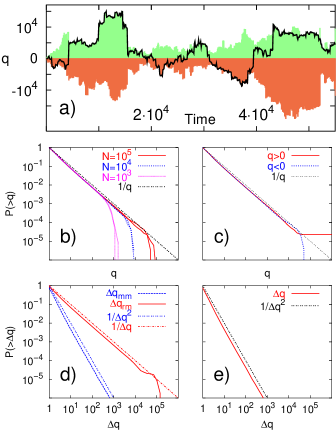
Figure 1: Main features of the basic model. In panel a) we show the development of the elements with largest positive $q_{max}$ and largest negative $q_{min}$ together with a particular trajectory, where we always follow the “winner” in the merging process (solid line). The simulation is done for a system of size $N=10^{4}$ elements, and the time-count is in updates per element. b-e) Cumulative plots of steady state properties. b) The size distributions of the positive and negative $q$ for 3 different system sizes. c) The size distribution when we start a system of size $N=10^{5}$ with initial condition $q_{i}=10$, $\forall i$. One observes that all excess $q$ is moved to a single element. d) Two variants of a histogram of size changes. $\Delta q_{mm}$ is defined by following the winner, meaning that we plot the difference in size between the largest of $q_{i},q_{j}$ before merging and the merged unit after the merging. $\Delta q_{rm}$ corresponds to the change from any of the two $q_{i},q_{j}$ to the merged unit. e) The size of changes defined as the losses of absolute $q$ in merging events where $q_{i}$ and $q_{j}$ are of different signs.

The main features obtained numerically are presented in Fig. 1. Fig. 1(a) illustrates the steady state after a transient time $\sim N$ updates per element, starting from an initial “vacuum” with $q_{i}=0,\forall i=1,2,...N$. The figure shows the extreme range of $q$-values at any time. The subsequent dynamics of the extremes is also reflected in the trajectory of a winner-element which, when merged, is re-identified as the merged element. One observes that this winning element exhibits an intermittent dynamics with size-changes $\Delta q$ of all magnitudes. The distribution of these changes as well as a wide set of other properties is in fact scale invariant. The cumulative distribution of $q$-values, Fig. 1(b), is a scale-free distribution,

$$P(>\!\!q)=\int_{q}^{\infty}P(q^{\prime})\mathrm{d}q^{\prime}\propto q^{1-\gamma},$$ (3)

with $\gamma=2$. With asymmetric initial condition, say $q_{i}=10,\forall i=1,2,...N$, as illustrated in Fig. 1(c), the system self-organizes by concentrating all of the initial asymmetry to one of the elements. All other elements are distributed in exactly the same way as with the “vacuum” initial condition (compare Figs. 1(b) and 1(c)).

Fig. 1(d) shows the distribution of changes in $\Delta q$ under steady state conditions. There are two possible ways to characterize these changes. One may quantify them by considering the difference between the merged element ($q_{i}+q_{j}$) and any of the two $q_{i}$ or $q_{j}$ merging elements. In that case one observes a cumulative distribution for changes $P(>\!\!\Delta q)=1/(\Delta q)$, (compare full drawn line and dashed line in Fig. 1(d)). This distribution closely resembles the overall distribution of $q$ values. Alternatively one may quantify the dynamics by following the winner at each merging, thus defining the $\Delta q$ as the difference between the largest $q$ before and the largest $q$ after the merging. In that case one expects the probability of change of size $\Delta q$

$$P_{change}(\Delta q)= P(q_{i}=\Delta q)\cdot P(q_{j}>\Delta q)$$

$$+ P(q_{j}=\Delta q)\cdot P(q_{i}>\Delta q)$$

$$\propto \frac{1}{\Delta q^{\gamma}}\frac{1}{\Delta q^{\gamma-1}}\;=\;\frac{1}{\Delta q^{2\gamma-1}},$$ (4)

which with $\gamma=2$ from Fig. 1(b) predicts exponent $3$ verified by simulations, see Fig. 1(d). Finally Fig. 1(e) shows the size-distribution of annihilation events, defined as events where two elements of different signs merge. The distributions of these annihilations are governed by the same considerations as in Eq. 4, and accordingly scales with exponent $\tau=3$.

Now we explore the reason for the $\gamma=2$ scaling behavior. We consider the version of the model where one excites the system by randomly picking a zero element and assigning it a $+/-$ value:

$$q_{i} \rightarrow q_{i}+q_{j}$$ (5)

$$q_{j} \rightarrow r$$ (6)

were $r$ is a random number picked from a symmetric narrow distribution $F(q)$. This update is one of many possible versions that all produce the same scaling results as shown in Fig. 1, we here consider it because it is the simples to treat analytically. The differential equation, describing the evolution of the model reads takayasu ; takayasu2

$$\frac{dP(q)}{dt}= \iint_{\!\!\!-\infty}^{\infty}\mathrm{d}q_{2}\mathrm{d}q_{1}\delta(q-q_{1}-q_{2})P(q_{1})P(q_{2})$$ (7)

$$- 2P(q)+F(q),$$

which have been shown to give a steady state distribution with the asymptotic behaviour $P(q)\propto 1/q^{2}$ takayasu . For pedagogical reasons we here present an alternative solution, that also opens for some insight into the amazing robustness of this model. In terms of the Fourier transform $p(\omega)=\int\mathrm{d}qe^{-iq\omega}P(q)$ the steady state equation is

$$p(\omega)=1-\sqrt{1-f(\omega)}.$$ (8)

The important property is that $p(\omega)-1\propto-|\omega|$ for small $\omega$. A positive creation probability $F(q)$ with a finite second moment ensures this which leads to $P(q)\propto q^{-2}$ for large $q$. Thus the exponent $2$ will be a common property for a large class of variations of the basic merging and creation mechanism. As an example $F(q)=\exp(-|q|)/2$ gives

$$P(q)=\frac{1}{\pi}-\frac{1}{\pi}\operatorname{Re}[S_{11}(iq)]=\frac{1}{\pi q^{2}}-\frac{3}{\pi q^{4}}+\cdots,$$ (9)

where $S_{11}(z)$ is a Lommel function and $P(k=0)=1/\pi$. Also the localization of positive excess $\langle q\rangle N$ can be understood, since a symmetric $F(q)$ implies an even continuum solution and thus that all excess will occupy a zero $q$ measure around $q_{0}=\langle q\rangle N$. For a discrete simulation this means a single $q$ as illustrated in Fig. 1c.

Finally, for application in real physical situations, it is also of interest to explore the behaviour of the merging-and-creation scenario in finite dimensions. As was reported by takayasu ; takayasu2 ; krapivsky then the observed scaling $1/q^{2}$ is robust, even when we confine the elements to diffusive motion in 1 dimension, provided that creation of +/- pairs occur close to each other. For a visualization of the dynamic behaviour we in Fig. 2 show the evolving system in 1-d.

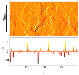
Figure 2: Merging and creation in 1-dimension: At each time-step one selects a coordinate $i$ between 1 and N=100. If $q_{i}=0$, one create a $+/-$ pair at position $i$ and one of its neighbors. If $q_{i}\neq 0$ then one moves $q_{i}$ one step to either left or right and adds it to the $q$ already present at that position. In upper panel one sees the time evolution over in total 100 updates per site, whereas the lower panel is a snapshot of the final configuration. One may notice that merging of light (positive) and dark (negative) sites leads to annihilation of both. The steady state distribution of $q$ is scale invariant with the same exponent 2 as in the basic (infinite dimensional) model.

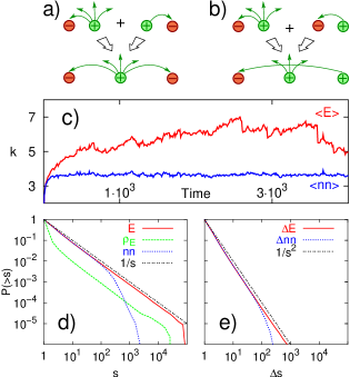
Figure 3: The network realization of the model. a) and b) illustrate possible merging moves. Positive vertices (donors) are vertices with outgoing edges and negative (acceptors) with incoming edges. c) The dynamics of the average number of edges per node, $\langle E\rangle$, (upper curve) and the average number of neighbors $\langle nn\rangle$ (lower curve), $N=10^{4}$. d) The cumulative probability distributions, $N=10^{5}$, for: number of edges incoming or outgoing from a node, $E$ (solid curve); number of neighbors, $nn$ (dotted curve); edge density, $\rho_{E}$ defined as the number of parallel edges connecting two vertices (dashed curve). The distributions for all quantities are scale-free $P(>\!\!s)\sim 1/s^{\gamma-1}$ with $\gamma=2$. e) The cumulative probability distributions for the changes in number of edges due to merging, $\Delta E$ and number of neighbors $\Delta nn$. The distributions are power-law $P(>\!\!\Delta s)\sim{\Delta s}^{1-\tau}$ with exponent $\tau=2\gamma-1=3$ from Eq. 4.

We now consider a network implementation where each element is a vertex and its sign corresponds to the number of in- or out-edges. Thus the above scenario is translated to a network model in which donor ($q>0$) and acceptor ($q<0$) vertices are connected by directed edges, see Fig. 3(a) and (b). Each vertex may have different number of edges, but at any time a given vertex cannot be both donor and acceptor. Further, in the direct generalization of the model, we allow several parallel edges between any pair of vertices. At each time-step two vertices $i$ and $j$ are chosen randomly. The update is then:

• Merge the two random vertices $i$ and $j$. There are now two possibilities:
  a) If they have the same sign all the edges from $i$ and $j$ are assigned to the merged vertex. Thereby the merged vertex has the same neighbors as $i$ and $j$ had together prior the merging, see Fig. 3(a).
  b) If $i$ and $j$ have different signs, the resulting vertex is assigned the sign of the sum $q_{i}+q_{j}$. Thereby a number $max\{|q_{i}|,|q_{j}|\}-|q_{i}+q_{j}|$ of edges are annihilated in such a way that only the two merging vertices change their number of edges. This is done by reconnecting donor vertices of incoming edges to acceptor vertices of outgoing edges, see Fig. 3(b).

• One new vertex is created of random sign, with one edge being connected to a randomly chosen vertex.

On the vertex level this network model can be mapped to the above model for merging and creation, and thus predict similar distributions of vertex sizes, as seen by comparing solid line in Fig. 3(d) with Fig. 1(b) and distributions of annihilations in Fig. 3(e) and Fig. 1(e). However, the network formulation provides additional insight into the excitation process that drives the whole distribution. That is, starting with a number of empty vertices $q_{i}=0$, the creation process generates vertex antivertex pairs on small scale which subsequently may grow and shrink due to merging and creation as illustrated in Fig. 3(c). One can see, that when the system has reached the stationary state, the average number of neighbors $\langle nn\rangle$ is nearly constant with small fluctuations while the fluctuations in the average number of edges, $\langle E\rangle$, are much larger. Further one notices that the evolution of $\langle E\rangle$ is asymmetric, in the sense that increases are gradual, while decreases are intermittent with occasional large drops in $\langle E\rangle$. These drops primarily correspond to the merging of vertices of different signs, where a large number of edges may be annihilated. This process is quantified in Fig. 3(e).

The network model opens for a new range of power-laws hughes associated to the connection pattern and dynamics of reconnections between the vertices. In this connection it is interesting that the number of edges per vertex, $E$, is distributed with scaling $P(E)\propto 1/E^{2}$. This was also obtained for the “number of loops at foot-point” in hughes . In addition, the distribution of reconnection events $P_{\Delta}(\Delta E)\propto 1/\Delta E^{3}$ is distributed as the “flare energies” in the model of Ref. hughes . In our model the event size is simply the change in the number of edges ($\Delta E$) when two vertices merge which gives the exponent -3 as shown in Eq. 7. In the model of Hughes et al. hughes the event size is a more complex quantity related to cascades of crossings of field lines, and the energy release is associated to the number of lines that thereby decrease their length. The non trivial fact that we obtain the same exponent suggests that the two models are in the same universality class, which means that our minimalistic model captures the main features of a presumably much larger class of more detailed and realistic models.

Also we would like to mention that the distribution of the number of parallel edges for connected pairs of nodes is also scale invariant $P(>\!\!\rho_{E})\propto\rho_{E}^{1-\gamma}$ see Fig. 3(d). This illustrates robustness of the mechanism: The dynamics of merging vertices appears very different when it is viewed from the “dual” space of tubes of edges between vertices, $\rho_{E}$, nevertheless the same exponent $\gamma=2$ is obtained.

In conclusion we have discussed a new mechanism for obtaining scale-free networks of connected donor and acceptor vertices. The model predicts power-laws of node degrees with a $1/s^{2}$ distribution, and of reconnection events with a $1/\Delta s^{3}$ distribution. The scenario thus provides a generic framework to generate networks with large-scale features from small-scale excitations under steady state conditions, and may thus complement preferential growth which provides scaling only under persistently growing conditions gronlund . Viewed as SOC, the merging-creation scenario provides “scaling for free” in the sense that it is robust to multiple simultaneous updates. The key process of both constructive (equal sign) merging and destructive (opposite sign) merging ala should be an important ingredient in a number of dynamic systems, and in particular appears to be appealing minimalistic model with possible connection to reconnection and creation of solar flares.

References

- (1) M. Paczuski and D. Hughes, cond-mat/0311304 (2003).
- (2) R. Close, C. Parnell, D. MacKay and E. Priest, Sol. Phys. 212 251 (2003).
- (3) M.J. Aschwanden et al. Astrophys. J. 535, 1047 (2000).
- (4) E. Parker, Astrophys. J. 390, 290 (1992).
- (5) D. Hughes, M. Paczuski, R.O. Dendy, P. Helander and K.G. McClements. Physical Rev. Letters 90 131101 (2003).
- (6) M. Faloutsos, P. Faloutsos, and C. Faloutsos, Comput. Commun. Rev. 29, 251 (1999).
- (7) A.-L. Barabasi, R. Albert (1999). Emergence of scaling in random networks, Science, 286, 509.
- (8) A. Broder et al. (2000). B. Kumar, F. Maghoul, P. Raghavan, S. Rajagopalan, R. Stata, A. Tomkins, J. Wiener, Graph Structure in the Web, Computer Networks 33, 309-320.
- (9) H. Simon (1955). Biometrika 42 (1955) 425.
- (10) P. Bak, C. Tang and K. Wiesenfeld, Phys. Rev. Lett. 59 (1987) 381-374.
- (11) P. Bak, K. Chen and C. Tang, Phys. Lett. 147 297 1990.
- (12) P. Bak and K. Sneppen, Phys Rev. Lett. 71 (1993) 4083.
- (13) H. Takayasu, Phys. Rev. Lett. 63 2563, (1989)
- (14) H. Takayasu, M. Takayasu, A. Provata and G. Huber, J. Stat. Phys. 65, 725 (1991).
- (15) P.L. Krapivsky, Physica A 198, 157 (1993).
- (16) A. Gronlund, K. Sneppen and P. Minnhagen, cond-mat/0401537.
- (17) In fact even and generates a distribution apart from one continuously growing giant component that takes care of the non-conservation in this particular update.