Freezing of Nonlinear Bloch Oscillations in the Generalized Discrete Nonlinear Schrödinger Equation

Abstract

The dynamics in a nonlinear Schrödinger chain in an homogeneous electric field is studied. We show that discrete translational invariant integrability-breaking terms can freeze the Bloch nonlinear oscillations and introduce new faster frequencies in their dynamics. These phenomena are studied by direct numerical integration and through an adiabatic approximation. The adiabatic approximation allows a description in terms of an effective potential that greatly clarifies the phenomena.

I Introduction

The study of the generalized discrete nonlinear Schrödinger (GDNLS) equation, introduced by Salerno salerno as a model providing one-parametric transition between discrete nonlinear Schrödinger (DNLS) equation and exactly integrable Ablowitz-Ladik (AL) model AL , is attracting increasing interest, due to the relevance of lattice dynamics in various fields of physics, as condensed matter, fiber optics physics, molecular biology (see e.g. Scott and references therein) and recently Bose-Einstein condensate (see e.g AKKS and references therein).

One of the most interesting phenomena, which can be observed in the different discretizations of the nonlinear Schrödinger equation is the so-called Bloch oscillations, that appear when a linear force is applied to a solitary wave solution. Such oscillations in the integrable AL model with a linear force have been discovered in BLR , numerically found in the DNLS Scharf , and interpreted as Bloch oscillations, using the analogy with the solid state physics, in KCV . Later on, Bloch oscillations were studied in the GDNLS equation CaiElectric and in the presence of impurities KonoAdiabatic . Bloch oscillations have been observed experimentally in an array of waveguides array , found also to exist in the case of a dark soliton kondark and in a totally discretized (i.e. discrete-time discrete space) nonlinear Schrödinger equation kondisc

In the present article we report some peculiarities of the Bloch oscillations of bright solitons in the GDNLS equation. More specifically we show that the model preserves the Bloch oscillations, the amplitude of which however displays in certain cases an abrupt change when the parameter governing transition between AL and DNLS models is changed.

Section II presents the model, i.e., the GDNLS equation with discrete translational invariant integrability-breaking terms in an external homogenous electric field, and the soliton initial conditions considered for this model. In Section III we present the adiabatic approximation, that will prove to be very useful to understand the dynamics. It allows a description in terms of an effective potential. In Section IV we describe the main ingredients of the dynamics: the Bloch oscillations and the freezing of the Bloch oscillations, and provide an explanation of this features in terms of the adiabatic effective potential. Finally, in the conclusions (Section V), we summarize the main results and discuss their relevance.

II The model

The equation of motion for the system we are dealing with reads

$$i\frac{d\psi_{n}}{dt}+(1+|\psi_{n}|^{2})(\psi_{n+1}-\psi_{n-1})-2\chi n\psi_{n}-\nu(\psi_{n+1}+\psi_{n-1}-2\psi_{n})|\psi_{n}|^{2}=0\;.$$ (1)

where $\nu$ is the integrability-breaking parameter providing one-parametric transition between the AL model AL ($\nu=0$) and the DNLS model ($\nu=1$), and $\chi$ is a parameter defining the strength of the linear force. In particular, at $\nu=0$ Eq. (1) is integrable and has the exact bright soliton solution KCV

$$\psi_{n}(t)=\frac{\sinh(2\,w)\;\exp\left\{i\left[{\frac{\cosh(2\,w)\sin(2\,\chi\,t)}{\chi}}-2\,\chi\,nt\right]\right\}}{\cosh\left\{2\,w(n-\xi_{0})-{\frac{\sinh(2\,w)\left[\cos(2\,\chi\,t)-1\right]}{\chi}}\right\}}$$ (2)

where $w$ and $\xi_{0}$ are constant parameters of the solutions ($\xi_{0}$ can be interpreted as the initial position of the soliton center, and $1/w$ as the soliton width).

Our purpose is to study how the $\nu$-term changes the soliton evolution; i.e., we consider the evolution for $\nu\neq 0$ of initial conditions of the form

$$\psi_{n}(0)={\frac{\sinh(2\,w)}{\cosh[2\,w(n-\xi_{0})]}}$$ (3)

III Adiabatic approximation

Let us start with the analysis of the problem when it is close to integrable, i.e., when $|\nu|\ll 1$. We employ the perturbation theory (in the presence of a linear force it was developed in KonoAdiabatic ) and limit ourselves to the adiabatic approximation. This means that the term $\nu(\psi_{n+1}+\psi_{n-1}-2\psi_{n})|\psi_{n}|^{2}$ is considered as a perturbation of the AL model. As we have previously seen, for $\nu=0$ there are exact solutions of the form

$$\psi_{n}=-i\frac{\sinh(2w)\,e^{-2i\theta(n-\xi)+i\varphi}\,e^{-i(2n+1)\chi t}}{\cosh[2w(n-\xi)]}\;.$$ (4)

In the adiabatic approximation we compute the time evolution of the parameters $w$, $\xi$, $\theta$ and $\varphi$; while keeping the functional form of Eq. (4) fixed. The equation of motion (1) can be written as

$$i\frac{d\psi_{n}}{dt}+(1+|\psi_{n}|^{2})(\psi_{n+1}-\psi_{n-1})-2\chi n\psi_{n}=\nu(\psi_{n+1}+\psi_{n-1}-2\psi_{n})|\psi_{n}|^{2}\;.$$ (5)

with the $\nu$-term considered as a perturbation. This approach gives the following evolution equations for the parameters

$$\frac{d\theta}{dt} = A(w,\xi)\,\cos[2(\chi t+\theta)]+B(w,\xi)$$ (6)

$$\frac{d\xi}{dt} = C(w,\xi)\,\sin[2(\chi t+\theta)]$$ (7)

$$\frac{dw}{dt} = D(w,\xi)\,\sin[2(\chi t+\theta)]$$ (8)

where

$$A(w,\xi) = \frac{\nu}{2}\,\sinh^{4}(2w)$$ (11)

$$\times\sum_{n=-\infty}^{\infty}\frac{\sinh[2w(n-\xi)]}{\cosh[2w(n+1-\xi)]\cosh^{2}[2w(n-\xi)]\cosh[2w(n-1-\xi)]}$$

$$\quad\quad\quad\quad\times\left\{\frac{1}{\cosh[2w(n+1-\xi)]}+\frac{1}{\cosh[2w(n-1-\xi)]}\right\}$$

$$B(w,\xi) = -\nu\,\sinh^{4}(2\,w)$$ (13)

$$\times\sum_{n=-\infty}^{\infty}{\frac{\sinh[2w(n-\xi)]}{\cosh[2w(n+1-\xi)]\cosh^{3}[2w(n-\xi)]\cosh[2w(n-1-\xi)]}}$$

$$C(w,\xi) = -\frac{\sinh(2\,w)}{w}\left(1+\frac{\nu}{2}\,\sinh^{3}(2\,w)\right.$$ (16)

$$\times\left.\sum_{n=-\infty}^{\infty}\frac{(n-\xi)}{\cosh[2w(n+1-\xi)]\cosh[2w(n-\xi)]\cosh[2w(n-1-\xi)]}\right.$$

$$\quad\quad\quad\quad\times\left.\left\{\frac{1}{\cosh[2w(n+1-\xi)]}-\frac{1}{\cosh[2w(n-1-\xi)]}\right\}\right)$$

$$D(w,\xi) = -\frac{1}{2}\,\nu\,\sinh^{2}(2\,w)$$ (19)

$$\times\sum_{n=-\infty}^{\infty}\frac{1}{\cosh[2w(n+1-\xi)]\cosh[2w(n-\xi)]\cosh[2w(n-1-\xi)]}$$

$$\quad\quad\quad\quad\times\left\{\frac{1}{\cosh[2w(n+1-\xi)]}-\frac{1}{\cosh[2w(n-1-\xi)]}\right\}\;.$$

From these expressions one can see that the coefficients $A$, $B$, $C$ and $D$ are periodic in $\xi$ with period $1$. The dynamics of $\theta$, $\xi$ and $w$ is decoupled from the evolution of the phase $\varphi$, and $\varphi$ is merely slaved to the dynamics of the previous parameters. We have seen numerically that for a wide range of parameters $A(w,\xi)=0$ and $D(w,\xi)=0$ (for $\xi$ integer of halfinteger it is easy to prove it analytically using that the terms of the series are odd-functions in $n$), therefore the adiabatic equations of motion reduce to

$$\frac{d\theta}{dt} = B(w,\xi)$$ (20)

$$\frac{d\xi}{dt} = C(w,\xi)\,\sin[2(\chi t+\theta)]$$ (21)

$$\frac{dw}{dt} = 0\;.$$ (22)

The corrections in $B$ and $C$ due to the $\nu$-term, $B/\nu$ and $[C+\sinh(2w)/w]/\nu$ [Eqs. (13)-(16)], are plotted in Fig. 1 for various values of $w$. One can see that $B/\nu$ is $\xi$-dependent and takes greater values for narrower solitons. On the other hand, the corrections in $C$ coming from the $\nu$-term are greater for wider solitons, and are nearly $\xi$ independent.

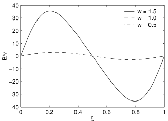
Figure 1: (a) $B/\nu$ and (b) $[C+\sinh(2w)/w]/\nu$ as a function of $\xi$ for various values of $w$.

In the previous equations we can make the change of variable $\alpha\equiv\chi t+\theta$, after this change it results a system of autonomous differential equations for $\alpha$ and $\xi$

$$\frac{d\alpha}{dt} = \chi+B(\xi)$$ (23)

$$\frac{d\xi}{dt} = C(\xi)\sin(2\alpha)\;.$$ (24)

The differential equation for the orbits is

$$\frac{d\alpha}{d\xi}=\frac{\chi+B(\xi)}{C(\xi)\sin(2\alpha)}\;,$$ (25)

that gives the equation for the orbits $\alpha=\alpha(\xi)$. Deriving with respect to time Eq. (24) and substituting the equation for the orbits, $\alpha=\alpha(\xi)$, we obtain a second order evolution equation for $\xi$ in terms of an effective force, $F_{eff}$, that only depends on $\xi$,

$$\frac{d^{2}\xi}{dt^{2}} = F_{eff}(\xi)$$ (26)

$$F_{eff}(\xi) = \frac{dC(\xi)}{d\xi}\,C(\xi)\sin^{2}[2\alpha(\xi)]+2C(\xi)[\chi+B(\xi)]\cos[2\alpha(\xi)]\;.$$ (27)

This evolution equation (multiplying by $d\xi/dt$ and integrating over time) leads to the energy conservation law

$$\frac{1}{2}\left(\frac{d\xi}{dt}\right)^{2}+V_{eff}(\xi)=constant\;,$$ (28)

$$V_{eff}(\xi)=-\int_{0}^{\xi}\!d\xi^{\prime}\,F_{eff}(\xi^{\prime})\;,$$ (29)

where $V_{eff}$ is the effective potential. Thus, the soliton in the adiabatic approximation can be seen as a particle moving in an effective potential. This interpretation is very useful to understand the Bloch oscillations and its freezing.

IV Dynamics in the presence of the $\nu$-term

The evolution of soliton initial states of the form

$$\psi_{n}={\frac{\sinh(2\,w)}{\cosh[2\,w(n-\xi_{0})]}}$$ (30)

is characterized by two main phenomena: the Bloch oscillations and its freezing.

IV.1 Bloch oscillations

The evolution of these states present dynamical localization in the form of Bloch oscillations, see Fig. 2 (as in the $\nu=0$ case Scharf ). This phenomenon is a consequence of the discreteness of the system.

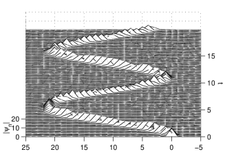
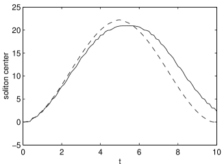
Figure 2: (a) Bloch oscillations of a soliton [full evolution, Eq. (1)] in a Schrödinger chain with $\nu=-0.01$. (b) Dynamics of the center of the soliton [adiabatic approximation, Eqs. (6)-(8)] for $\nu=-0.01$ (full line) and for $\nu=0$ (dashed line). Both figures with initial conditions $w_{0}=1.5$, $\xi_{0}=0$ and $\theta_{0}=0$, in external field $\chi=-0.3$.

The dynamical localization can be understood in the adiabatic approximation (see Eq. 29). This approximation predicts that the soliton center position, $\xi$, feels a trapping effective potential (see Fig. 3), and the turning points of the motion are for $2(\chi t+\theta)$ multiple of $\pi$ (see Eq. 21). The adiabatic approximation gives good results for the amplitude and the period of the Bloch oscillations, and we also observe that the soliton width ($1/w$) remains approximately constant as the adiabatic approximation predicts.

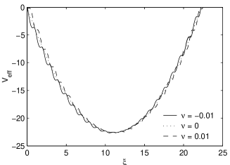
Figure 3: Effective adiabatic potential for a soliton with initial conditions $w_{0}=1.5$, $\xi_{0}=0$ and $\theta_{0}=0$ in a Schrödinger chain with an external field $\chi=-0.3$ for various values of $\nu$.

The $\nu$ term changes the period and amplitude of the Bloch oscillations, and introduces new (fast) frequencies in the dynamics [Fig. 2]. These differences can be seen as a consequence of the changes in the adiabatic effective potential, see Fig. 3. For $\nu>0$ the lattice sites have an effective attractive interaction for the soliton center; thus the effective potential displays local minima near the lattice sites. Conversely for $\nu<0$ the effective interaction is repulsive, and the local minima are located in the intersite regions.

The evolution of the center of the soliton is correctly predicted by the adiabatic approximation (Eqs. (20)-(22)) at early times. Later the effects of the radiative decay and the change of shape of the soliton became important, and the description of these effects falls beyond the scope of the adiabatic approximation. These nonadiabatic effects become more important for increasing $|\nu|$. Another phenomenon that cannot be studied within the adiabatic approximation is the emergence of chaotic behavior chaos , the adiabatic approximation do not account of this effect because it reduces the computation of the evolution to the integration of the conservation law in Eq. (28).

IV.2 Freezing of the Bloch oscillations

The main new phenomenon reported in this article is the freezing of the Bloch oscillations due to an homogeneous integrability breaking term (the $\nu$-term). This freezing is a trapping of the soliton in a lattice site (or in a intersite region), that happens in a region of the parameter space [Fig. 4]. This is an intrinsic localization effect due to characteristics of the lattice chain, not a localization induced by lattice inhomogeneities KonoAdiabatic .

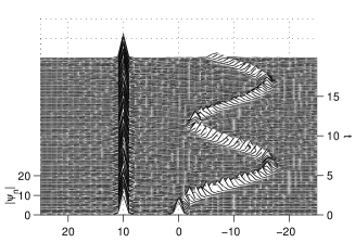
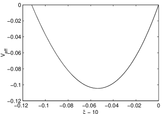
Figure 4: (a) Narrow soliton ($w_{0}=1.5$ and $\xi_{0}=10$); and wide soliton ($w_{0}=1.3$ and $\xi_{0}=0$) evolutions in a Schrödinger chain with $\nu=0.02$ in an external field $\chi=0.3$, both with $\theta_{0}=0$. (b) Effective adiabatic potential for the narrow soliton.

The freezing of the Bloch oscillations can be easily explained in the adiabatic approximation, where it corresponds to the center of the soliton variable being trapped in a local minimum of the effective potential. See Fig. 4.

Therefore, in the case $\nu>0$, the freezing emerges for solitons centered near lattice sites (and with $d\xi/dt\simeq 0$); while in the case $\nu<0$, it emerges when the soliton center is near the middle of an intersite region. In both cases the phenomena is favored for narrow solitons (greater $w$), strong $\nu$-terms (greater $\nu$) and weaker external fields (smaller $|\chi|$). See Fig. 5.

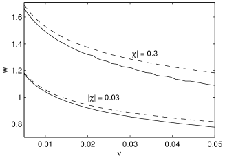
Figure 5: Bloch oscillations are frozen in the regions above the curves for values of the external field smaller than those indicated in the curves (taking for the other parameters $\theta_{0}=0$ and $\xi_{0}=0$). Full lines: computation with the complete equations of motion. Dashed lines: computation with the adiabatic approximation.

The parameter region predicted by the adiabatic approximation [Eqs. (6)-(8)] is in good agreement with the results of the numerical evolution of the full equation of motion [Eq. (1)]. However, the adiabatic approximation is not able to describe the unfreezing at early times, that can only be observed when the parameters are very close to the limit of the freezing region [Fig. 6]. The reason is that this unfreezing is related to non-adiabatic effects (change of the soliton shape and radiation).

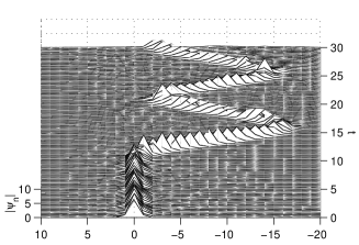
Figure 6: Dynamical defrosting due to nonadiabatic effects (radiation and change of soliton shape) of a soliton with initial conditions close to the frozen-unfrozen limit in parameter space. $w_{0}=1.2633$, $\xi_{0}=0$ and $\theta_{0}=0$ in a Schrödinger chain with an external field $\chi=0.3$ for $\nu=0.025$.

V Conclusions

These results show that inhomogeneity in the lattice is not required to freeze the Bloch oscillations, i.e., to trap the soliton in a region with a size of the order of the intersite distance in the lattice. We show that the discrete translational invariant integrability-breaking term that makes the transition between AL and DNLS models can freeze the nonlinear Bloch oscillations, i.e., gives rise to an intrinsic localization. This phenomenon can be understood as the trapping of the soliton center position in a minimum of the effective potential that we obtain in the collective variable or adiabatic approximation. The integrability-breaking terms considered, the $\nu$-term, produces an effective attractive (for $\nu>0$) or repulsive (for $\nu<0$) interaction with the lattice sites, that gives rise to local minima in the effective potential where the soliton can be trapped. This $\nu$-term has also the effect of changing the main frequency of the Bloch oscillation and introducing faster new frequencies in the dynamics, that can also be understood as a consequence of the change in the effective potential.

These new phenomena show a richer dynamics of the DNLS equation, increasing the interest and potential applications of this model, and they also suggest the possibility of other new effects in the presence of time varying external forces.

References

- (1) M. Salerno, Phys. Rev. A46, 6856 (1992).
- (2) M. Ablowitz and J. Ladik, J. Math. Phys. 16, 598 (1975); and, 17, 1011 (1976).
- (3) A.C. Scott, Nonlinear Science, Oxford University Press (1999).
- (4) G. L. Alfimov, P. G. Kevrekidis, V. V. Konotop and M. Salerno, Phys. Rev. E66, 046608 (2002).
- (5) M. Bruschi, D. Levi and O. Ragnisco, Nuovo Cimento A53, 21 (1979).
- (6) R. Scharf, A. R. Bishop, Phys. Rev. A43, 6535 (1991).
- (7) V. V. Konotop, O. A. Chubykalo, L. Vazquez, Phys. Rev. E48, 563-568 (1993).
- (8) D. Cai, A. R. Bishop, N. Gronbech-Jensen, M. Salerno, Phys. Rev. Lett. 74, 1186 (1995).
- (9) V. V. Konotop, D. Cai, M. Salerno, A. R. Bishop, N. Gronbech-Jensen, Phys. Rev. E53, 6476 (1996).
- (10) R. Morandotti, U. Peschel, J. S. Aitchison, H. S. Eisenberg, Y. Silberberg, Phys. Rev. Lett. 83, 4756 (1999). T. Pertsch, P. Dannberg, W. Elflein, A. Bräuer, F. Lederer, Phys. Rev. Lett. 83, 4752 (1999).
- (11) V. V. Konotop Teor. Mat. Fiz. 99, 413 (1994).
- (12) V. V. Konotop, Physics Letters A258, 18-24 (1999).
- (13) D. M. McLaughlin, C. M. Schober, Physica D 57, 447 (1992).
- (14) D. H. Dunlap and V. M. Kenkre, Phys. Rev. B34, 3625 (1986).