Lagrangian statistics in fully developed turbulence

Abstract

The statistical properties of fluid particles transported by a fully developed turbulent flow are investigated by means of high resolution direct numerical simulations. Single trajectory statistics are investigated in a time range spanning more than three decades, from less than a tenth of the Kolmogorov timescale up to one large-eddy turnover time. Acceleration and velocity statistics show a neat quantitative agreement with recent experimental results. Trapping effects in vortex filaments give rise to enhanced small-scale intermittency on Lagrangian observables.

The knowledge of the statistical properties of particle tracers advected by a fully developed turbulent flow is a key ingredient for the development of stochastic Lagrangian models in such diverse contexts as turbulent combustion, pollutant dispersion, cloud formation and industrial mixing P94 ; Pope ; S01 ; Y02 . Given the importance of this problem, there are comparatively few experimental studies of turbulent Lagrangian dispersion. Progress in this direction has been hindered mainly by the presence of a wide range of dynamical timescales, an inherent property of fully developed turbulence. Indeed, in order to obtain an accurate description of the particle statistics it is necessary to follow their paths with very high resolution, i.e., well below the Kolmogorov timescale $\tau_{\eta}$, and for a long time lapse – of the order of an eddy turnover time $T_{L}$. The ratio of these timescales can be estimated as $T_{L}/\tau_{\eta}\sim R_{\lambda}$ where the microscale Reynolds number $R_{\lambda}$ ranges in the hundreds for typical laboratory experiments. A recent breakthrough has been made by La Porta et al LVCAB01 ; VLCBA02 who, borrowing techniques from high-energy physics, were able to track three-dimensional trajectories with a resolution of $0.05\tau_{\eta}$ and thus to study the statistics of particle acceleration. However, owing to the small measurement volume, trajectories could be followed only up to a few $\tau_{\eta}$, preventing any investigation of the long time correlations along particle paths. Conversely, the acoustical technique adopted by Mordant et al MMMP01 enabled them to successfully track particles for durations comparable to $T_{L}$ but could not access time delays of the order of $\tau_{\eta}$, and was restricted to one-dimensional measurements. More conventional techniques, e.g. based on CCD cameras OM00 , reveal useful only for moderate Reynolds numbers ($R_{\lambda}\simeq 100$) due to their limitations in the acquisition rate. In addition, all laboratory techniques require a considerable amount of signal processing to get rid of experimental noise. Besides these drawbacks, increasing difficulties are met when attempting to deal with multi-particle tracking.

In the light of the above remarks Direct Numerical Simulation of fully developed turbulence represents a valuable alternative tool for the investigation of Lagrangian statistics RP74 ; YP89 ; SE91 ; Y91 ; VY99 ; BS02 ; IK02 ; CRLMPA03 ; SYBVLCB03 and its important contribution has been recently reviewed in Ref. Y02 . Nonetheless, computational approaches have to face three demanding requirements: (i) have the largest possible value of $R_{\lambda}$ in order to maintain the flow in a fully developed turbulent state; (ii) resolve properly the dissipative scales with the aim of computing accurately small-scale observables; (iii) follow particle trajectories for times comparable to a large-eddy-turnover time. High resolution and huge computational resources are therefore needed to accomplish such a goal, making massive parallel computing by far and away the most appropriate tool. In this Letter we report the results of Direct Numerical Simulations of Lagrangian transport in homogeneous and isotropic turbulence on the parallel computer IBM-SP4 at CINECA, on $512^{3}$ and $1024^{3}$ cubic lattices with Reynolds numbers up to $R_{\lambda}\sim 280$, a very accurate resolution of dissipative scales, and a long integration time $T\approx T_{L}$. The Navier-Stokes equations

$$\partial_{t}{\bm{u}}+{\bm{u}}\cdot{\bm{\nabla}}{\bm{u}}=-{\bm{\nabla}}p+\nu\Delta{\bm{u}}\;,$$ (1)

are integrated on a triply periodic box by means of a fully dealiased pseudospectral code (the numerical parameters are listed in Table 1).

$R_{\lambda}$	$u_{rms}$	$\varepsilon$	$\nu$	$\eta$	$L$	$T_{L}$	$\tau_{\eta}$	$T$	$\delta x$	$N^{3}$	$N_{p}$
183	1.5	0.886	0.00205	0.01	3.14	2.1	0.048	5	0.012	5123	0.96$\cdot 10^{6}$
284	1.7	0.81	0.00088	0.005	3.14	1.8	0.033	4.4	0.006	10243	1.92 $\cdot 10^{6}$

Table 1: Parameters of the numerical simulations. Microscale Reynolds number $R_{\lambda}$, root-mean-square velocity $u_{rms}$, energy dissipation $\varepsilon$, viscosity $\nu$, Kolmogorov lengthscale $\eta=(\nu^{3}/\varepsilon)^{1/4}$, integral scale $L$, large-eddy turnover time $T_{L}=L/u_{rms}$, Kolmogorov timescale $\tau_{\eta}=(\nu/\varepsilon)^{1/2}$, total integration time $T$, grid spacing $\delta x$, resolution $N^{3}$, and the number of Lagrangian tracers $N_{p}$.

Energy is injected at an average rate $\epsilon$ by keeping constant the total energy in each of the first two wavenumber shells CDKS93 . With the present choice of parameters the dissipative range of lengthscales is extremely well resolved. With regard to the scaling properties of the velocity field, our results are in perfect numerical agreement with previous numerical simulations at comparable $R_{\lambda}$ (see e.g. KIYIU03 ). Upon having reached statistically stationary conditions for the velocity field, millions of Lagrangian tracers have been seeded into the flow and their trajectories integrated according

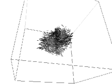
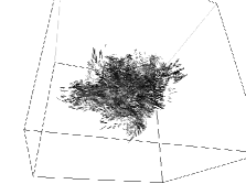
Figure 1: Snapshots of a subset of Lagrangian particles ( $\approx 12000$) at three different times $t=(0.2,0.5,0.8)T_{L}$. Gray scales encode different velocity amplitudes.

to

$$\frac{d{\bm{X}}}{dt}={\bm{u}}({\bm{X}}(t),t)\;,$$ (2)

over a time lapse of the order of $T_{L}$ (See Fig. 1). Particle positions ${\bm{X}}(t)$ and velocities ${\bm{v}}(t)=\dot{\bm{X}}(t)$ have been stored at a sampling rate $0.07\tau_{\eta}$. The forces acting on the particle – pressure gradients ${\bm{\nabla}}p({\bm{X}}(t),t)$ , viscous forces $\nu\Delta{\bm{u}}({\bm{X}}(t),t)$ and external input – and the resulting particle acceleration ${\bm{a}}(t)=\dot{\bm{v}}(t)$ have been recorded along the particle paths every $0.14\tau_{\eta}$. The resulting database permits detailed study of the statistics of Lagrangian velocity and acceleration over a range of timescales spanning more than three decades.

In what follows, we will focus on the description of the statistics of single particle trajectories, deferring the discussion of multi-particle statistics to a forthcoming publication. The analysis reveals the presence of frequent entrapment events within vortical structures (see Fig. 2). The characteristic frequency of these spiraling paths is comparable to $\tau_{\eta}^{-1}$ and their duration can be as long as $10\tau_{\eta}$. The velocity experienced during these events can attain $5u_{rms}$ with an ensuing acceleration $5u_{rms}/\tau_{\eta}$ as large as $80a_{rms}$. As we will show below, these events have a significant impact on time correlations up to $10\tau_{\eta}$.

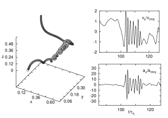
Figure 2: Trajectory and time series. Left panel: 3D trajectory of a trapping event in vortex filament. Acceleration and velocity fluctuations here reach about $30$ and $2$ r.m.s. values, respectively (right panels).

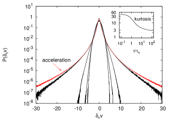
Figure 3: Probability density functions of velocity increments and acceleration, normalized with their variance. Curves refer to time increments $\tau=(97,25,6,0.7)\tau_{\eta}$ from inside to outside, and to the acceleration (outermost curve). In the inset, the kurtosis $K(\tau)=\left\langle{\delta_{\tau}v}^{4}\right\rangle/(\left\langle\delta_{\tau}v)^{2}\right\rangle^{2}$ for the entire time interval $0.07\tau_{\eta}\div 2T_{L}$. The saturation of $K(\tau)$ at small time increments is an indication of the high numerical resolution.

In Fig. 3 we present the probability density functions (PDFs) of velocity differences $\delta_{\tau}v=v(t+\tau)-v(t)$ taken along a given direction and rescaled by their variance $\langle(\delta_{\tau}v)^{2}\rangle^{1/2}$. For the shortest time delays shown in the figure the velocity increment PDF approaches the distribution of the acceleration $a(t)$ which is characterized by a strong intermittency, stretched exponential tails and a flatness $\langle a^{4}\rangle/\langle a^{2}\rangle^{2}\approx 40$. Classical Kolmogorov scaling arguments (see e.g. Ref. MY75 ) yield for the acceleration variance the prediction

$$\langle a^{2}\rangle=a_{0}\,\varepsilon^{3/2}\nu^{-1/2}\;.$$ (3)

We measure the constant $a_{0}=3.5\pm 0.3$, in agreement with the results of Ref. VY99 at comparable $R_{\lambda}$. Yet, one needs to notice that intermittent corrections may introduce in the definition of $a_{0}$ some dependency on Reynolds numberVLCBA02 . At larger time separations the PDFs are decreasingly intermittent and eventually become slightly sub-Gaussian for $\tau\approx T_{L}$, with a flatness $\langle(\delta_{\tau}v)^{4}\rangle/\langle(\delta_{\tau}v)^{2}\rangle^{2}\approx 2.8$. Assuming a scaling law for the second-order Lagrangian velocity structure function in the time-range $\tau_{\eta}\ll\tau\ll T_{L}$, dimensional analysis MY75 , predicts $\langle(\delta_{\tau}v)^{2}\rangle=C_{0}\varepsilon\tau$. Remark that this prediction is not affected by intermittency corrections owing to its linear dependence on the energy dissipation rate N89 ; B93 ; BDM02 . Therefore, $C_{0}$ is expected to be universal. For our data the scaling behavior holds on a relatively narrow window in $\tau$, leading to some uncertainty in the determination of the numerical prefactor. We estimate $C_{0}=5\div 6$, not far from previous measurements MMMP01 ; LD02 .

The intermittency in the PDFs of $\delta_{\tau}v$ can be conveniently quantified in terms of the Lagrangian velocity structure functions $S_{p}(\tau)=\langle(\delta_{\tau}v)^{p}\rangle$, that are expected to behave as power laws $\tau^{\xi_{p}}$. The scaling exponents $\xi_{p}$ can be evaluated by looking at the logarithmic slope $d\log S_{p}(\tau)/d\log\tau$ that should display a plateau in the range $\tau_{\eta}\ll\tau\ll T_{L}$. From Fig. 4 it is clear that it is very difficult to extract the values for $\xi_{p}$. However, by means of the extended self-similarity procedure BCTBMS93 , it is possible to estimate the relative exponents $\xi_{4}/\xi_{2}=1.7\pm 0.05$, $\xi_{5}/\xi_{2}=2.0\pm 0.05$, $\xi_{6}/\xi_{2}=2.2\pm 0.07$, in fair agreement with those obtained in Ref. MMMP01 . The range of time delays over which relative scaling occurs is $10\tau_{\eta}$ to $70\tau_{\eta}$. In this range anisotropic contributions induced by the large scale flow appear to influence the scaling properties.

It is interesting to remark that for values of $\tau$ in the range from $\tau_{\eta}$ to $10\tau_{\eta}$, the local slopes are significantly smaller and tend to accumulate around the value $2$ for all orders. This relevant correction to scaling cannot be attributed to the influence of the dissipative range $\tau<\tau_{\eta}$, since the latter would increase the value of the local slope, rather than decreasing it. A similar effect can be detected in Eulerian structure functions as well, yet the intensity in the latter case is much less pronounced. These strong deviations in the Lagrangian scaling laws are most likely due to the trapping events depicted in Fig. 2. Indeed, the long residence time within small-scale vortical structures introduces an additional weighting factor that enhances the effect with respect to Eulerian measurements.

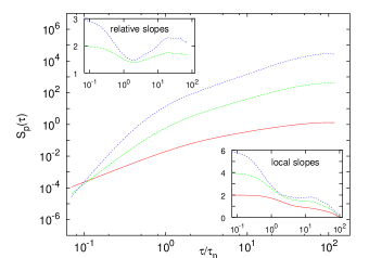
Figure 4: Log-log plot of Lagrangian structure functions of orders $p=2,4,6$ (bottom to top) vs $\tau$. Bottom right: logarithmic local slopes $d\log S_{p}(\tau)/d\log\tau$ (same line styles). Top left: relative local slopes with respect to the second order structure function $d\log S_{p}(\tau)/d\log S_{2}(\tau)$, for $p=4,6$. Data refer to the $v_{x}$ component. The two other velocity components exhibit slightly worse scaling due to anisotropy effects.

Further insight into the single particle dynamics can be gained by investigating the various force terms concurring to determine the total particle acceleration

$$\frac{d^{2}{\bm{X}}(t)}{dt^{2}}=-{\bm{\nabla}}p({\bm{X}},t)+\nu\Delta{\bm{u}}({\bm{X}}(t),t)+\bm{F}({\bm{X}}(t),t)\;.$$

As shown in the inset of Fig. 5, it is evident that the main source of acceleration is the pressure gradient VY99 , whereas the viscous term is important only near relatively strong acceleration events and the forcing contribution is negligible. A more quantitative test is given by the comparison of the PDFs of the three forces in Fig. 5.

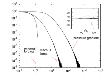
Figure 5: Log-log plot of PDFs for $-\partial_{x}p$, $\nu\Delta u_{x}$, $F_{x}$. The external forcing is virtually negligible, and the main contribution to large accelerations is made by pressure gradients. Inset: a typical evolution of the three terms along a particular trajectory. The strongest signal is $\partial_{x}p$ (dashed line), while the viscous force is activated only as a subleading response to pressure gradients (solid line). The force contribution is indistinguishable from zero.

To conclude, we have presented the analysis of single-particle statistics in high Reynolds number flows. Our results fit well with previous experimental measurements. At variance with experiments, we can investigate the statistical properties of millions of particles on a wide range of time intervals, from a small fraction of the Kolmogorov time up to the integral correlation time. We found clear indications that velocity fluctuations along Lagrangian trajectories are affected by multiple-time dynamics. In the interval $10\tau_{\eta}<\tau<T_{L}$ we observed anomalous scaling for Lagrangian velocity structure functions. For frequencies of the order of $\tau_{\eta}^{-1}$ we noticed that velocity fluctuations are affected by events where particles are trapped in vortex filaments. Events with trapping times much longer than expected on the basis of simple dimensional analysis appear frequently. The main novelty of Lagrangian single-particle velocity fluctuations with respect to Eulerian fluctuations is probably the capture of trajectories induced by small-scale structures. For example, the event analyzed in Fig. 2 would have a much smaller weight in an Eulerian analysis because of large-scale sweeping past the fixed probe. Among the most challenging open problems arising from our analysis are how to incorporate such dynamical processes in stochastic modelization of particle diffusion S01 and in the Lagrangian multifractal description B93 ; BDM02 .

- (1) S.B. Pope, Annu. Rev. Fluid Mech. 26, 23 (1994).
- (2) S.B. Pope, Turbulent Flows, Cambridge University Press (2000).
- (3) B. Sawford, Annu. Rev. Fluid Mech. 33, 289 (2001).
- (4) P.K. Yeung, Annu. Rev. Fluid Mech. 34, 115 (2002).
- (5) A. La Porta, G.A. Voth, A.M. Crawford, J. Alexander and E. Bodenschatz, Nature 409, 1017 (2001).
- (6) G.A. Voth, A. La Porta, A. Crawford, E. Bodenschatz and J. Alexander,. J. Fluid Mech. 469, 121 (2002).
- (7) N. Mordant, P. Metz, O. Michel and J.F. Pinton, Phys. Rev. Lett. 87, 214501 (2001).
- (8) S. Ott and J. Mann, J. Fluid Mech. 422, 207 (2000).
- (9) J.J. Riley and G.S. Patterson, Jr, Phys. Fluids 17, 292 (1974).
- (10) P.K. Yeung and S.B. Pope, J. Fluid Mech. 207, 531 (1989).
- (11) K.D. Squire and J.K. Eaton, Phys. Fluids A 3, 130 (1991).
- (12) P.K. Yeung, J. Fluid Mech. 427, 241 (1991).
- (13) P. Vedula and P.K. Yeung, Phys. Fluids 11, 1208 (1999).
- (14) G. Boffetta and I.M. Sokolov, Phys. Rev. Lett. 88, 094501 (2002).
- (15) T. Ishihara and Y. Kaneda, Phys. Fluids 14, L69 (2002).
- (16) L. Chevillard, S. G. Roux, E. Leveque, N. Mordant, J.F. Pinton and A. Arneodo, Phys. Rev. Lett. 91, 214502 (2003).
- (17) B.L. Sawford, P.K. Yeung, M.S. Borgas, P. Vedula, A. La Porta, A.M. Crawford and E. Bodenschatz, Phys. Fluids 15, 3478 (2003).
- (18) S. Chen, G. D. Doolen, R. H. Kraichnan and Z.-S. She, Phys. Fluids A 5, 458 (1993).
- (19) Y. Kaneda, T. Ishihara, M. Yokokawa, K. Itakura, and A. Uno, Phys. Fluids 15 L21 (2003).
- (20) A. Monin and A. Yaglom, Statistical Fluid Mechanics MIT Press, Cambridge, MA (1975), Vol. 2.
- (21) E.A. Novikov, Phys. Fluids A 1, 326 (1989).
- (22) M.S. Borgas, Phil. Trans. R. Soc. Lond. A, 342, 379 (1993).
- (23) G. Boffetta, F. De Lillo and S. Musacchio, Phys. Rev. E 66, 066307 (2002).
- (24) R.C. Lien and E.A. D’Asaro, Phys. Fluids 14, 4456 (2002).
- (25) R. Benzi, S. Ciliberto, R. Tripiccione, C. Baudet, F. Massaioli and S. Succi, Phys. Rev. E 48, R29 (1993).