“Clusterization” and intermittency of temperature fluctuations in turbulent convection

Abstract

Temperature time traces are obtained in turbulent thermal convection at high Rayleigh numbers. Measurements are made in the midplane of the apparatus, near the sidewall but outside the boundary layer. A telegraph approximation for temperature traces is generated by setting the fluctuation amplitude to 1 or 0 depending on whether or not it exceeds the mean value. Unlike the standard diagnostics of intermittency, the telegraph approximation allows one to distinguish the tendency of events to cluster (“clusterization”) from their large-scale variability in amplitude. A qualitative conclusion is that amplitude intermittency might mitigate clusterization effects.

I Introduction

We consider turbulent convection in a confined container of circular crosssection and 50 cm diameter. The aspect ratio (diameter/height) is unity. The sidewalls are insulated and the bottom wall is maintained at a constant temperature, which is higher by a small amount $\Delta T$ than that of the top wall. The working fluid is cryogenic helium gas. By controlling the temperature difference between the bottom and top walls, as well as the thermodynamic operating point on the phase plane of the gas, the Rayleigh number (Ra) of the flow could be varied between $10^{7}$ and $10^{15}$. We measure temperature fluctuations at various Rayleigh numbers towards the upper end of this range, in which the convective motion is turbulent. Time traces of fluctuations are obtained at a distance of 4.4 cm from the sidewall on the center plane of the apparatus. This position is outside of the boundary layer region for the Rayleigh numbers considered here. More details of the experimental conditions and measurement procedure can be found in Ref. NS1 .

A significant part of convection, even at the high Rayleigh numbers that concern us here, is due to plumes LK . We use the term here merely to denote an organized activity of convection without implying much about their three-dimensional shapes and sizes, or the parameters on which they scale, though a few comments will be made momentarily. The primary goal of the paper is to learn about the tendency of the plumes to cluster together (“clusterization”).

The upper part of Fig. 1 shows a short segment of temperature fluctuations at $Ra=1.5\times 10^{11}$. There are four large-scale events within this segment (marked by the letters A-D), and we imagine them to be the manifestation of large-scale plumes. Each event consists of several subevents, and there also exist a number of small events marked a-i. While it may well be that the subevents deserve to be considered separately, we regard them collectively here. Under these circumstances, it is clear that a typical life-time of the large events is of the order of 8 seconds. Noting from Ref. NS2 that the mean speed of the large-scale circulation (“mean wind”) for these conditions is about 6 cm/s, a typical length scale of these events is of the order of 50 cm, which is the characteristic dimension of the apparatus. That is, if these large-scale plumes originate from the boundary layer, it is as if the entire boundary layer on the bottom wall participates once in a while in this activity that we have called the large-scale plume. The maximum temperature in these large-scale plumes is a fraction of the excess temperature of the bottom plate (namely $\Delta T/2$), so, presumably, the fluid that is participating in the formation of a typical large-scale plume comes from the top parts of the boundary layer; or, if a plume does indeed come from the very bottom parts of the boundary layer, it is already partially mixed by the time it reaches the probe midway between the top and bottom walls. They are certainly not small-scale events that scale on the thickness of the boundary layer. This description does not apply to small-scale plumes a-i, though, presumably, they too belong to the same family. In Fig. 1, we show the case of hot plumes, that is, the case when the wind at the measurement point arrives from the hotter bottom plate. One can imagine that the wind direction could be just the opposite, leading to the arrival at the probe of cold plumes coming from the colder top plate. We have analyzed such instances as well. Further, beyond a certain Rayleigh number, as described in Ref. NS2 , the mean wind reverses itself randomly, so that a probe permanently held at one position sees hot plumes for some period of time and cold plumes for some other period of time. We have analyzed the two parts separately by stringing together only hot parts or the cold parts of a measured temperature trace. The data for the two cases have been examined separately. In each case, the telegraph approximation is related to specific properties of the underlying physical processes associated with hot or cold plumes, as they encounter the probe during their motion.

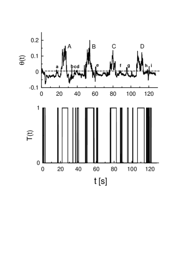
Figure 1: An example of the measured temperature time trace (upper part) and its random telegraph approximation (lower part). In addition to the small plumes marked a-i, there are several others such structures in the signals. They have not been marked merely because they occur below the zero line.

II Random telegraph approximation

A more detailed discussion of the plumes will be presented elsewhere but we limit ourselves here to a discussion of their tendency to cluster together occasionally. This is not obvious from the piece of the temperature trace shown in Fig. 1, and a longer trace crowds the plumes too much. It may be surmised that the clusterization is indeed responsible for the mean wind in the apparatus. In the usual methods of analysis of turbulent signals my , it is difficult to separate the clusterization effect from the usual intermittency effects arising from amplitude variability. To separate the two effects, we ignore the variation of the amplitude from one plume to another and replace the temperature trace of the type shown in the upper part of Fig. 1 by its random telegraph approximation, shown in the lower part. This approximation is generated from the measured temperature by setting the fluctuation magnitudes to 1 or 0 depending on whether the actual magnitude exceeds the mean value (marked as zero and shown by the dashed line in the upper part of Fig. 1). Formally, for the temperature fluctuation $\Theta(t)$ (with zero mean), the telegraph approximation $T(t)$ is constructed as

$$T(t)=\frac{1}{2}\left(\frac{\Theta(t)}{|\Theta(t)|}+1\right).$$

By definition, $T$ can assume either 1 and 0. The telegraph approximation can be generated by setting different “thresholds” than the mean. It turns out that most properties examined here are reasonably independent of the threshold; this comment will be made also at other specific places in the paper.

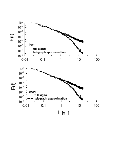
Figure 2: Spectra of the telegraph approximation of two realizations of the temperature trace compared with those of the temperature trace itself. The ordinate has been shifted so that the first points in both spectra coincide.

It may be useful to know how the conventional statistics for the random telegraph approximation compare with those of the temperature signal. Figure 2 compares the spectral densities, $E(f)$, of the telegraph approximations with those of the full signal. The comparisons are made separately for hot and cold cases. It is clear that the spectra of the telegraph approximation are close to those of the original signal in a significantly large interval of scales. The main difference is that the telegraph approximation is richer in spectral content above a certain frequency. This is not difficult to understand from a visual inspection of Fig. 1.

Of particular interest is the power-law behavior of the spectral densities of the telegraph approximation. For both hot and cold cases, they follow a power-law of the form

$$E(f)\sim f^{-\beta}.$$

Though this power-law behavior is clear from Fig. 2, we reproduce in Fig. 3 the spectra of the telegraph signal, computed from several records to attain better statistical convergence, in order to emphasize the power-law scaling. The exponent $\beta=1.38\pm 0.02$. A reasonable shift of the threshold does not change the spectral exponent $\beta$.

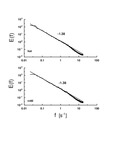
Figure 3: Spectrum in the telegraph approximation computed using twenty realizations of the temperature trace, for the hot case (upper plot) and for the cold case (bottom part). The straight lines (the best fit) show that the power-law approximation (2) holds well for both hot and cold cases.

From the closeness of the spectra of the temperature trace with its telegraph approximation, it is inferred easily that the former has a spectral exponent of 1.38 as well, albeit over a smaller range of scales. Observation of the temperature trace spectra with such power law was first made in lib , and was explored theoretically in y , and is now a well-known result.

The probability density function of the duration between events, $\tau$, for the telegraph approximation is shown in Fig. 4. Data for the hot and cold cases are given separately. The log-log scale has been chosen to emphasize the power-law structure

$$p(\tau)\sim\tau^{-\alpha}.$$

For both hot and cold cases, we observe $\alpha=1.37\pm 0.03$. A reasonable variation of the threshold in the vicinity of the average value does not change the exponent $\alpha$.

It is known that, for non-intermittent cases (Ref. jen and Sec. 4), the relation between the exponents $\alpha$ and $\beta$ is given by

$$\beta=3-\alpha.$$

If we substitute in (4) the value of $\alpha\simeq 1.37$ (as observed in Fig. 4) we obtain $\beta\simeq 1.63$. This is considerably larger than that actual value measured in Fig. 3, namely 1.38. This discrepancy is the object of interest to us here; as already remarked, since there are no amplitudes involved, it must be related to clusterization entirely (see also jen ).

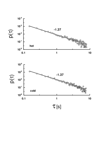
Figure 4: The probability density function of the duration $\tau$ for the telegraph approximation of the temperature signal (for hot and cold cases). The straight lines (the best fits) are drawn to indicate the scaling law (3).

It is of interest to note here that, for the telegraph approximation of the temperature fluctuation in the turbulent atmospheric boundary layer, we have about the same values of $\alpha$ and $\beta$ as the present, while the spectral density of the temperature trace has a roll-off rate of about 1.66 (consistent with the Kolmogorov-Obukhov-Onsager-Corrsin theory my ). It is clear that the spectra of the temperature signal and its telegraph approximation are closer in confined convection than in atmospheric turbulence.

III Quantifying clusterization

The difference between the observed telegraph spectral exponent ($\beta\simeq 1.38$) and its value given by Eq. (4) ($\simeq 1.63$) is a quantitative measure of clusterization jen of plume-like objects observed in temperature traces. This is a part of intermittency.

Intermittency of the so-called temperature dissipation rate my ,sa is characterized in turbulence by

$$\chi=|\frac{dT^{2}}{dt}|.$$

Following Obukhov my , the local average

$$\chi_{\tau}=\frac{1}{\tau}\int_{t}^{t+\tau}\chi(t)dt$$

can be used to describe the intermittency of $\chi$. The scaling of the moments,

$$\frac{\langle\chi_{\tau}^{q}\rangle}{\langle\chi_{\tau}\rangle^{q}}\sim\tau^{-\mu_{q}},$$

assuming that scaling exists, is a common tool for the description of the intermittency my ,sa . Intermittent signals possess a non-zero value of the exponent $\mu_{q}$. Of particular interest is the exponent $\mu_{2}$ for the second-order moment.

The telegraph approximation is a composite of Heaviside step functions, so the dissipation rate (5) is a composite of pulses (i.e. delta-functions) located at the edges of the boxes of the telegraph signal. For the uniform random distribution of the pulses along the time axis, $\mu_{q}=0$. Non-zero values of $\mu_{q}$ mean that there is a clusterization of pulses. Figure 5 shows dependence of the normalized dissipation rate $\langle\chi_{\tau}^{2}\rangle$ on $\tau$ for the telegraph approximation of hot and cold signals. The straight lines (the best fits) are drawn to indicate the scaling law (6), for $q=2$. It should be noted that scaling interval for the dissipation rate is the same as for the PDF and for the spectrum (cf. Figs. 3 and 4). Values of the intermittency exponent $\mu_{2}$, calculated as slopes of the straight lines in Fig. 5 is $\mu_{2}\simeq 0.47\pm 0.03$. The relatively large value of the exponent $\mu_{2}$ suggests that the clusterization of the pulses is quite strong.

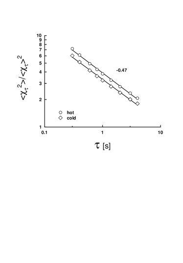
Figure 5: Normalized second moment of the local dissipation rate for the telegraph approximation plotted against $\tau$, for cold and hot cases. The straight lines (the best fits) are drawn to indicate the scaling law (6).

The temperature dissipation can be also characterized by the “gradient” measure my ,sa

$$\chi_{r}=\frac{\int_{v_{r}}(\bigtriangledown{T})^{2}dv}{v_{r}},$$

where $v_{r}$ is a subvolume with space-scale $r$ (for detailed justification of this measure, see Ref. my , p. 381 and later). The scaling law of the moments of this measure are important characteristics of the dissipation field sa . By Taylor’s hypothesis my , we can replace $dT/dx$ by $dT/\langle u\rangle dt$ (where $\langle u\rangle$ is the mean wind and $x$ is the coordinate along the direction of the wind), and can define the dissipation rate as

$$\chi_{\tau}\sim\frac{\int_{0}^{\tau}(\frac{dT}{dt})^{2}dt}{\tau},$$

where $\tau\simeq r/\langle u\rangle$. This, too, should follow the scaling relation (6).

This definition has a problem in the telegraph approximation because $dT/dt$ is composed of delta functions. Fortunately, one is interested in the scaling of the discrete representation of the dissipation field, given by

$$\chi_{\tau}\sim\sum_{n=1}^{\tau}(\Theta_{n+1}-\Theta_{n})^{2}/\tau,$$

where $n$ specifies an interval of space. This discrete definition of $\chi_{\tau}$ avoids the problem with delta functions. Obviously, for the telegraph signal, scaling exponents calculated for the pulse-defined dissipation, Eqs. (5)-(6), and for the discrete spike-like process are identical; this observation is not true for the original temperature $\Theta(t)$.

IV Clusterization and the spectrum

The spectrum of the telegraph approximation can be related to the probability distribution $p(\tau)$ through

$$E(f)=\int W(t)G(ft)p(t)dt,$$

where $G(ft)$ is a transform function and the weight function $W(t)$ is supposed to have a scaling form

$$W(t)\sim t^{\delta}.$$

Since the quantities $G(ft)$ and $p(t)dt$ are dimensionless, one can use dimensional considerations to find the exponent $\delta$ (cf. Ref. my ) through

$$W(t)\sim\langle\chi\rangle\cdot t^{2},$$

and the use of (2),(3) and (7); this yields relation (4).

To estimate the clusterization correction on the relation between scaling spectrum and $p(t)$, we should take into account two-point correlations in the telegraph signal. This can be characterized by the two-point correlation function $\xi(t)$. In a situation where the two-point correlation function exhibits the scaling behavior

$$\xi(t)\sim t^{-\gamma},$$

the correlation exponent $\gamma$ is the same as the exponent $\mu_{2}$. This is easily seen by the well-known result that the correlation dimension proc $D_{2}$ is related to $\gamma$ through

$$D_{2}=1-\gamma,$$

and to $\mu_{2}$ Ref. sa via

$$D_{2}=1-\mu_{2},$$

thus yielding $\gamma=\mu_{2}.$ To estimate the weight function $W(t)$ with the same dimensional considerations as above, and to take into account the two-point correlation (which characterizes clusterization), we replace $\langle\chi\rangle$ by

$$\langle\chi_{t}^{2}\rangle^{1/2}\sim t^{-\mu_{2}/2}.$$

Replacing (9) by

$$W(t)\sim\langle\chi_{t}^{2}\rangle^{1/2}\cdot t^{2},$$

we have

$$W(t)\sim t^{2-\mu_{2}/2}.$$

The corresponding correction of Eq. (4) is

$$\beta=(3-\mu_{2}/2)-\alpha.$$

Using the value of $\mu_{2}\simeq 0.47$ from Fig. 5 and the value $\alpha\simeq 1.37$ from Fig. 4, we obtain

$$E(f)\sim f^{-1.40},$$

which compares well with the behavior found in Fig. 3 (see also lib ,y ).

V Summary and discussion

The results discussed so far are for a fixed Rayleigh number. The same situation seems to occur at other Rayleigh numbers. For those Rayleigh numbers where there is a reversal of the wind, the concatenated data corresponding to one given direction of the wind follow the same statistics as well. Thus, the characteristics discussed in the paper are generally valid for turbulent temperature fluctuations at all Rayleigh numbers covered in the measurements. The main conclusion is that the telegraph approximation captures the main statistical features of the temperature time trace obtained in convection. This approximation, which gives a clear separation between clusterization and magnitude intermittency, has been useful in demonstrating that there is a significant tendency for the plumes to cluster together. The telegraph approximation turns out to be useful here because of the specific process of heat transport, which is determined in large measure by the random motion of temperature plumes. However, one can expect that this approximation (or its modifications) may be also useful in the description of other turbulent signals. The exponent $\mu_{2}$ for the telegraph approximation, completely determined by clusterization, is about 0.47. This should be compared with the intermittency exponent computed for the $\chi$-$\chi$ correlation of the full temperature signal, which is about 0.36—consistent with similar estimates available for passive scalars (see, e.g., Ref. pms ). The clusterization exponent is thus larger than the classical intermittency exponent. From this, one can infer that the magnitude intermittency plays a smoothing role on the clusterization effects within the scaling interval.

We thank L.J. Biven, J. Davoudi and V. Yakhot for useful discussions.

References

- (1) J.J. Niemela and K.R. Sreenivasan, J. Fluid Mech. 481, 355 (2003).
- (2) L. Kadanoff, Phys. Today 54, 34 (2001).
- (3) K.R. Sreenivasan, A. Bershadskii, and J.J. Niemela, Phys. Rev. E 65, 056306 (2002); J.J. Niemela and K.R. Sreenivasan, Europhys. Lett. 62, 829 (2003).
- (4) A.S. Monin and A.M. Yaglom, Statistical Fluid Mechanics, Vol. 2, (MIT Press, Cambridge 1975).
- (5) M. Sano, X.Z. Wu and A. Libchaber, Phys. Rev. A 40, 6421 (1989).
- (6) V. Yakhot, Phys. Rev. Lett. 69, 769 (1992).
- (7) H.J. Jensen, Self-organized Criticality (Cambridge University Press, Cambridge, England, 1998).
- (8) K.R. Sreenivasan and R.A. Antonia, Annu. Rev. Fluid Mech, 29, 435 (1997).
- (9) P. Grassberger and I. Procaccia, Phys. Rev. Lett. 50, 346 (1983).
- (10) R.R. Prasad, C. Meneveau and K.R. Sreenivasan, Phys. Rev. Lett. 61, 74 (1988).